Machine Learning-Based Approaches for Predicting SPAD Values of Maize Using Multi-Spectral Images

Abstract

Precisely monitoring the growth condition and nutritional status of maize is crucial for optimizing agronomic management and improving agricultural production. Multi-spectral sensors are widely applied in ecological and agricultural domains. However, the images collected under varying weather conditions on multiple days show a lack of data consistency. In this study, the Mini MCA 6 Camera from UAV platform was used to collect images covering different growth stages of maize. The empirical line calibration method was applied to establish generic equations for radiometric calibration. The coefficient of determination (R²) of the reflectance from calibrated images and ASD Handheld-2 ranged from 0.964 to 0.988 (calibration), and from 0.874 to 0.927 (validation), respectively. Similarly, the root mean square errors (RMSE) were 0.110, 0.089, and 0.102% for validation using data of 5 August, 21 September, and both days in 2019, respectively. The soil and plant analyzer development (SPAD) values were measured and applied to build the linear regression relationships with spectral and textural indices of different growth stages. The Stepwise regression model (SRM) was applied to identify the optimal combination of spectral and textural indices for estimating SPAD values. The support vector machine (SVM) and random forest (RF) models were independently applied for estimating SPAD values based on the optimal combinations. SVM performed better than RF in estimating SPAD values with R² (0.81) and RMSE (0.14), respectively. This study contributed to the retrieval of SPAD values based on both spectral and textural indices extracted from multi-spectral images using machine learning methods.

1. Introduction

The unmanned aerial vehicle (UAV) mounted with multi-sensors has attracted great attention for the easy deployment, flexibility, and high temporal (daily) and spatial (centimeter-levels) resolutions in ecological and environmental domains [1,2,3,4].Compared with satellite platforms, UAVs are generally labelled as being light weight, with optional flying altitude, flexible dates for data acquisition, and easy deployment [5,6,7,8]. Therefore, UAVs are gradually becoming an alternative tool to satellite remote sensing in several applications, such as modelling, mapping, and monitoring biophysical parameters of vegetations in ecology, rangelands, forests, and agriculture [9,10,11,12,13]. UAVs mounted with multi-sensors are commonly applied to acquire high resolutions images for crop phenotyping of breeding and quantifying crop biophysical parameters variability for site-specific management in precision agriculture (PA) [14,15,16,17,18]. UAV remote sensing can be used in various agricultural aspects, such as predicting the soil and plant analyzer development (SPAD) values of canopy, detecting water stress, measuring crop’s canopy temperature, and predicting agricultural yields [19,20,21,22]. The high-throughput data, such as the high spatial resolution of multi-spectral images, provide great potentials in optimizing agronomic management of input to maximize crop yields and quality in PA [23,24,25].

The multi-spectral images can hardly be directly used to retrieve the physiological parameters of vegetation (forests and crops), as the original digital number (DN) contained both atmospheric effects and camera noise [26,27]. The statistical-based empirical line calibration method (ELCM) was commonly applied to calibrate the sensors mounted on satellites by reducing the atmospheric effects and converting the DN into reflectance. Commonly, two or more calibration targets of different gray levels were deployed, and the relationship between DN and reflectance was assumed to be linear [28]. With the development of UAV technology, the ELCM was widely applied in calibrating multi-spectral images acquired from UAV platforms. The detailed processing workflow containing data collection, pre-processing, radiometric calibration, and image classification based on the Mini MCA-6 Camera (MMC, Tetracam, Inc., Chatsworth, CA, USA) from a fixed-wing UAV was proposed and shown [29]. The radiometric calibration of a multi-spectral sensor with several calibration targets using ELCM was simplified, and achieved high accuracy [30]. The radiometric calibration using both artificial and natural objects were applied by a vicarious method [31]. However, the images were mostly acquired on a single day in mentioned studies, of which the climatic condition merely changed during the data acquisition. Therefore, there remained uncertainties in the synchronous measurement of reflectance due to accidental errors (measurement error from observation) and rapid changes of climatic variables (weather conditions and solar radiation). Thus, there is a need to test the effectiveness of the generic equations using the images collected on multi-days with the ELCM.

Various spectral indices (SIs) such as the normalized difference vegetation index (NDVI) and near-infrared reflectance of vegetation (NIRv) were widely used to investigate the plant’s physiological status, such as the nitrogen and CC, as well as the green leaf biomass and gross primary production (GPP) at large scales [32,33,34,35]. The textural indices (TIs) referred to the spatial variations of image greyscale levels as a function of scale, which were very helpful in improving the accuracy in image classification, image segmentation, change detection, yield prediction, and pattern cognition [36,37,38]. Combining SIs and TIs has great potential in interpreting features in pixel-based classification [39,40]. The SIs and TIs were combined to estimate the leaf area index (LAI) of rice, and results showed the combination of both texture and spectrum improved the prediction accuracy [41]. The potential performance of added textural information for image classification using the object-based image analysis (OBIA) techniques was tested, and achieved relatively high accuracy [42]. So far, textural information’s potential ability to monitor the growth condition of crops was rarely reported and kept unknown. Meanwhile, previous studies mainly used the data collected on limited growth stages of crops. Therefore, there is a need to assess the ability of combining the SIs and TIs for monitoring the growth condition of crops covering the entire growth stages.

The SPAD-502 chlorophyll meter (SPAD-502, Spectrum Technologies, Inc., Plainfield, IL, USA) was commonly applied to measure SPAD values, of which the values were proven to have correlated with the growth condition of crops and forests [1,43,44,45,46]. The readings of SPAD values can reflect the growth condition of vegetation in a direct way, of which high values indicated healthy growth of the plants [1,11]. The limited samples of SPAD values combined with near-surface UAV remote sensing can be applied for a large scale with high accuracy [47]. The relationships between plot-level SIs derived from UAV images and ground measured data, such as LAI and SPAD values, were calculated and compared, and the difference of these at two different rice growth stages were discussed and analyzed [48]. Shu et al. improved the estimation accuracy of SPAD values by removing the backgrounds from UAV hyper-spectral images [49]. The SPAD values of winter wheat was estimated using the cluster-regression method based on UAV hyper-spectral data [50]. New indices were proposed to predict SPAD values based on UAV RGB images for naked barley leaves [51]. The measurement of SPAD values provided effective and stable methods for identifying the crop phenotyping. The SPAD values have the potential to be converted into physiological parameters such as leaf chlorophyll content [52].

In this study, the ELCM was applied to obtain generic equations for the radiometric calibration of multi-spectral images acquired on different growth stages of maize. The hypothesis of this study was that the radiometric calibration using the generic equations was still effective, and thus, the indices (Sis and Tis) calculated based on well calibrated images will better catch the dynamic growth status of maize. The combined indices (spectral and textural indices) will help to improve the accuracy of predictions of SPAD values with advanced machine learning approaches at different growth stages of maize [53,54]. Therefore, the objectives of this study were to (1) generate and validate the generic equations for radiometric calibration of MMC; (2) investigate the potential ability of spectral indices, textural indices, and combined spectral and textural indices for predicting SPAD values at different growth stages of maize; and (3) scale up the estimations of SPAD values for maize using two machine learning approaches.

2. Materials and Methods

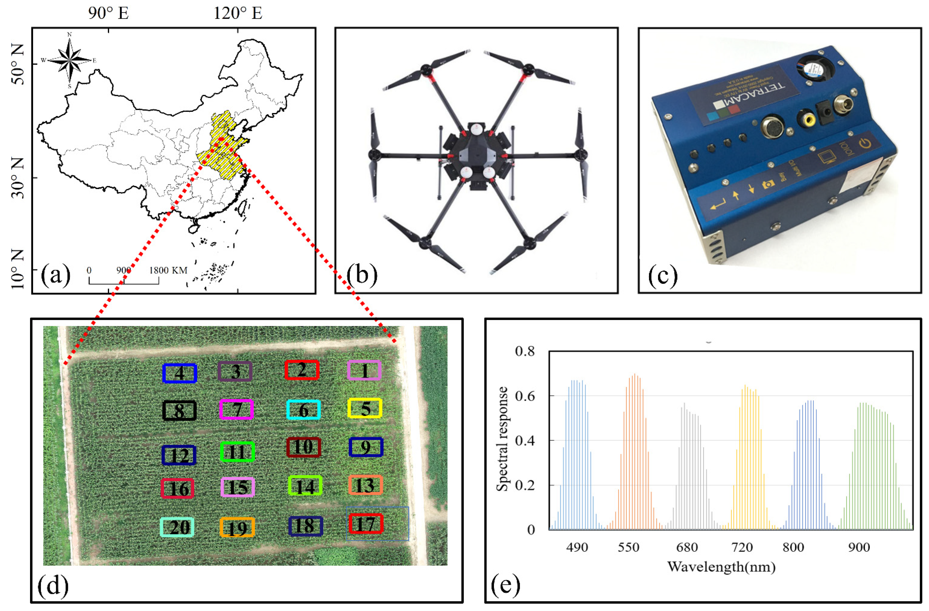
2.1. Study Area

The data collection was conducted in Nanpi Eco-Agricultural Experimental Station (NEES) (38.00° N, 116.40° E) (Figure 1). The site was initially built in the year 1982 by the Chinese Academy of Sciences (CAS) to explore the sustainable development of agriculture in North China Plain (NCP). For the current experimental design, there were 20 plots cultivated with the same maize cultivar (Zhengdan 958), treated by different varieties and amounts of fertilizers including nitrogen (N), phosphate (P), and potassium (K) in 2019. Each plot measured 10 m long and 8 m wide to avoid the disturbance from the side plot. The total amount of fertilizers for each plot was equally divided into three parts, one third was applied around ten days after crop emergence, another one third was applied at the booting date, and the last one third was applied at the tasseling date. The detailed information of fertilizers was given in

Table A1. The conduction of NPK fertilizers in 20 plots. The number in the table indicates the series number of the plots. The N fertilizer was urea, P fertilizer was calcium phosphate, and K fertilizer was potassium chloride. The numbers under the plots are the series number of plots. The number after the N, P, K represents the applied amounts of the fertilizers, and 1 indicates the 30 kg/ha.

Plots	Fertilizers	Plots	Fertilizers	Plots	Fertilizers	Plots	Fertilizers
1	N1P1K2	2	N3P1K1	3	N3P3K1	4	N2 + wheat + straw
5	N1P1K1	6	N3P3K2	7	N3P2K1	8	N2 + Organic material
9	N1P2K1	10	N2P2K2	11	N4P3K1	12	N3 + wheat-straw
13	N1P3K1	14	N2P1K1	15	N4P2K1	16	N3 + Organic material
17	N2P3K1	18	N2P2K1	19	N4P1K1	20	N4P2K2

in Appendix A. The management practices such as pest and weed control were strictly performed by professional workers under a standard procedure.

The DJI M600 Pro UAV platform (https://www.dji.com/cn/matrice600-pro, Shenzhen, China, accessed on 10 August 2021) equipped with Mini MCA 6 Camera (MMC) (http://www.tetracam.com/Products-Micro_MCA.htm, Tetracam Inc., Chatsworth, CA, USA, accessed on 10 August 2021) was applied for data collection. The system was used to collect images concerning 20 plots at different growth stages of maize (Figure 1b,c). The center wavelengths (full width at half maximum) of MMC were 490 (10), 550 (10), 680 (10), 720 (10), 800 (20), and 900 (10) nm for six bands, respectively. The relative monochromatic response filter transmission and peak transmission wavelength of each filter are displayed in Figure 1e. The MMC was proven to be very useful in generating maps of vegetation indices for assessing the water stress at the crown level due to the narrow bands [55,56]. The camera was very effective in evaluating the rangeland environments by classifying shrub canopies and grass patches using object-based image classification approach [29]. The camera was also applied in PA for monitoring the growth of maize by calculating NDVI [57].

For this study, two reflectance panels of 5% (0.6 × 0.6 m) and 60% (1.2 × 1.2 m) reflectance were used as black and white calibration targets, respectively. The contrast ratio of these two targets was (60/5 = 12), which was suitable for radiometric calibration [23]. These panels were relatively flat, the reflectance was uniform in all directions, and these panels can be deemed as Lambertian targets (Figure 2).

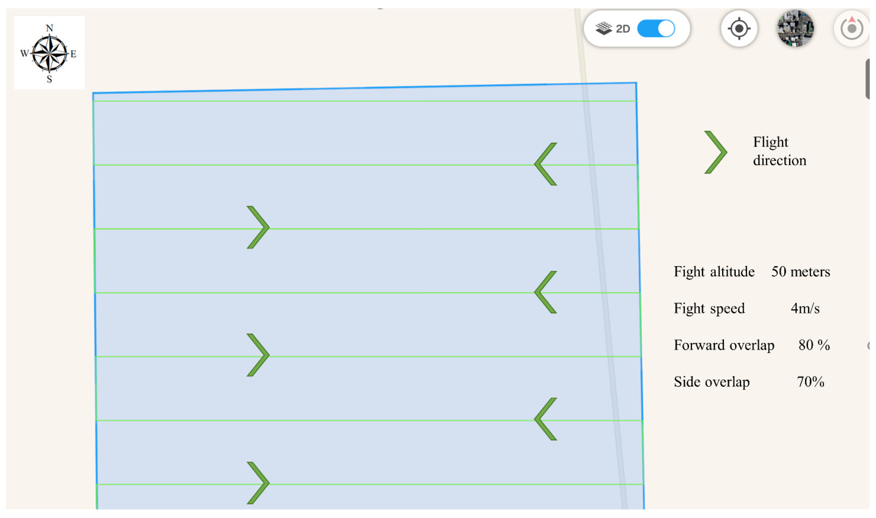
2.2. Data Collection

The UAV data covering the entire growth stages of maize were collected between 11:30 to 12:30 AM (Beijing time) to minimize changes in solar zenith angle in cloudless weather conditions. The important phenological events of maize, including the tasseling date (18 August), silking (25 August), blister (7 September), milk (15 September), physiological maturity (21 September), and maturity (30 September), were selected for data collection in the year 2019. For each flight, the altitudes and the speeds were strictly controlled as 50 m and 4 m/s, respectively. Each flight’s forward and side overlaps were set as 80 and 70%, and the detailed information of trajectory of UAV flight routes weraree clearly shown in Figure A1. The detailed locations of four ground control points (GCPs) were measured using the real-time kinematic (RTK) S86T system with fixed solutions (

Table 1. The detailed geo-location information of the ground control point (GCP) measured using the real-time kinematic (RTK) S86T system. The columns each present the locations of the GCP, and fixed solutions indicate the measurement was stable. The rows each represent the series number of the GCP.

	Latitude (°)	Longitude (°)	Height (m)	Fixed Solution
GCP 1	38.0156966331	116.6801892261	1.434	yes
GCP 2	38.0155875386	116.6794440042	1.530	yes
GCP 3	38.0149917169	116.6794959572	1.487	yes
GCP 4	38.0149398778	116.6802395461	1.316	yes

, Figure A2) [11]. The original RAW images were converted into single TIFF images, and then six single TIFF images of each shot were converted into one big multi-tiff image within PixelWrench2 Software (PW2, Tetracam Inc., Chatsworth, CA, USA) [29]. The orthophoto containing six multi-spectral bands was generated within Pix4D Mapper, based on the stacked images (Lausanne, Switzerland). The orthophotos acquired from different growth stages of maize were selected using the same region of interest (ROI) for each plot within Exelis ENVI (version 5.3, http://www.exelisvis.com, accessed on 15 August 2021) [58,59,60,61].

The panels were pre-set before each flight, and the reflectance was measured using ASD Handheld-2 (ASD-HH2, ASD Inc., Boulder, CO, USA, http://www.asdi.com/, accessed on 16 September 2021) shortly after the flight mission. The ASD Handheld-2 can measure reflectance ranging from 325 to1075 nm with spectral resolution being 1 nm [24]. To ensure the high accuracy of the spectrum collection, the measurement of reflectance was performed within 15 min after each flight. The reflectance of maize in 20 plots was independently collected on 5 August and 21 September 2019 for validation. Since the different spectrum resolutions of bands for MMC and ASD-HH2, there is a need to resample the narrow spectrum resolution of ASD-HH2 to make data consistent, fitting the wide spectrum resolution of MMC. The spectrum resampling was processed using the following equation:

$$R_e=\frac{{{\displaystyle \int }}_{{\lambda }_1}^{{\lambda }_2}{\rho }_{\lambda }{S}_{\lambda }{d}_{\lambda }}{{{\displaystyle \int }}_{{\lambda }_1}^{{\lambda }_2}{S}_{\lambda }{d}_{\lambda }}$$

(1)

where ${\lambda }_1$ and ${\lambda }_2$ are the maximum and minimum wavelengths of each band, $S_{\lambda }$ is the spectral response at wavelength $\lambda$, and ${\rho }_{\lambda }$ is the reflectance of calibration target at wavelength $\lambda$, respectively [31,62]. The $d_{\lambda }$ is the difference of signal of each wavelength (λ).

The SPAD values of maize in each plot were measured using SPAD-502Plus (Spectrum Technologies, Inc., Plainfield, IL, USA). A total of five sampling points were conducted at four corners and center in each plot. For each sampling, three strains of maize were randomly selected for the measurement of SPAD values using SPAD-502Plus [63,64]. There were 15 SPAD values in each plot, and the average values were calculated to be representative. This procedure was applied for data collection during the entire growth stages of maize.

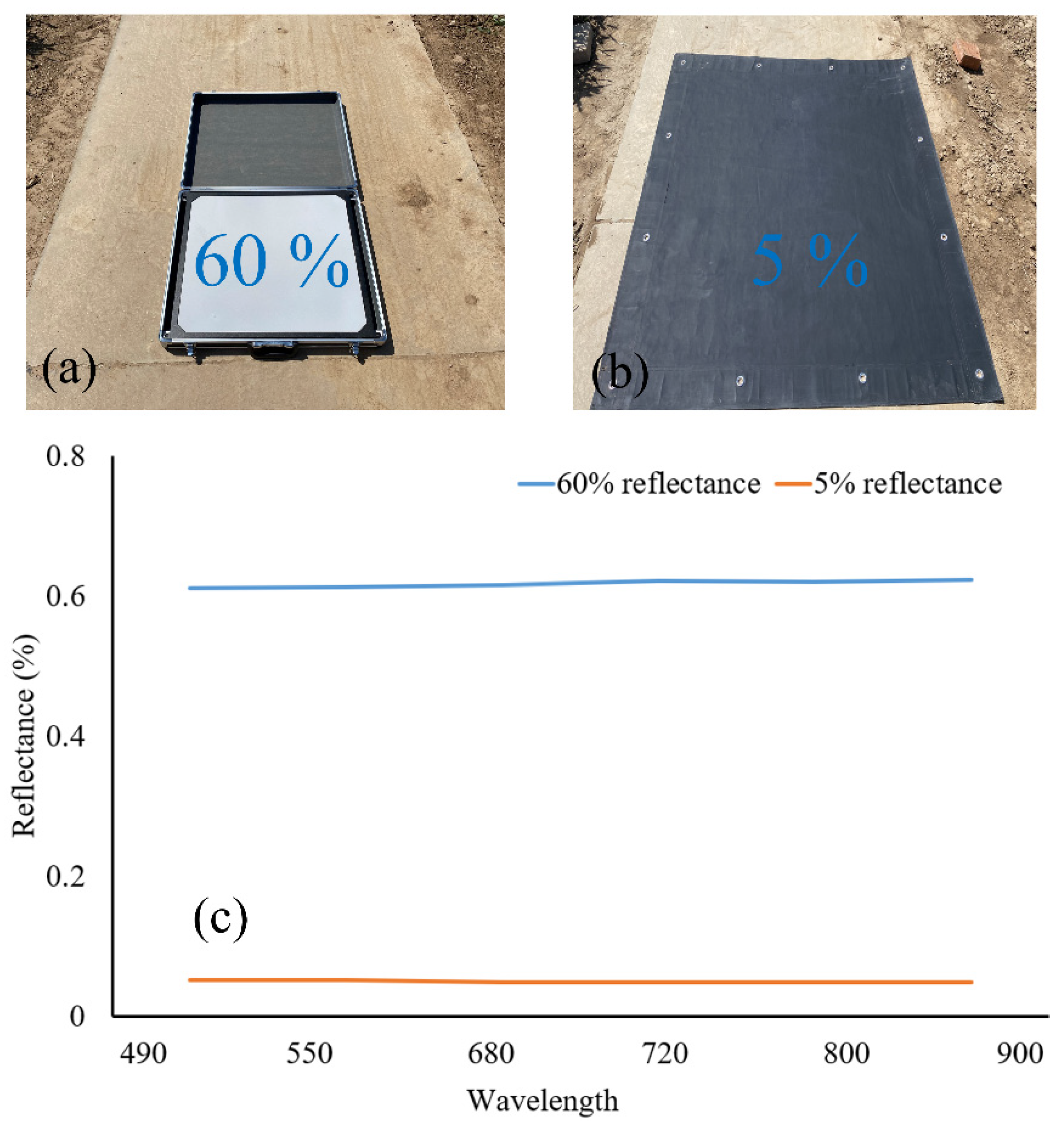
2.3. Radiometric Calibration of Multi-Spectral Images

For the radiometric calibration, the DN and reflectance of calibration targets of all dates were applied to obtain the generic equations. Firstly, the ROI covering 18 × 18 pixels at the center of calibration targets were made within ENVI5.3. Secondly, the average DN of the calibration targets within the ROI of the entire growing season were applied to plot against in-situ reflectance. Then, the ELCM was applied to confirm a line that can best fit all points as follows:

Reflectance = k × DN ± intercept

(2)

where the Reflectance was the reflectance of calibration targets, and k and DN (in 8 bit format) each represent the inherent properties of MMC, and the intercept is composed of systematic noise and atmospheric effects [23,65]. Through this method, the generic equation was independently confirmed for each band of the camera. Thirdly, the radiometric calibration was conducted by applying the generic equations to the original images.

For validation, the reflectance of maize was compared from calibrated images and from ASD-HH2 on 5 August, 21 September, and on both days. The accuracy was assessed by calculating the coefficients of determination (R², Equation (3)), the root mean square error (RMSE, Equation (4)), and the normalized root mean square error (NRMSE, Equation (5)), respectively.

$${\mathrm{R}}^2=\frac{{{\displaystyle \sum }}_{i=1}^n\left(M_i-\overline{M}\right)\left(P_i-\overline{P}\right)}{\sqrt{{{\displaystyle \sum }}_1^n{\left(M_i-\overline{M}\right)}^2-{{\displaystyle \sum }}_1^n{\left(P_i-\overline{P}\right)}^2}}$$

(3)

$$\mathrm{RMSE}=\sqrt{\frac{1}{n}{{\displaystyle \sum }}_1^n{\left(P_i-M_i\right)}^2}$$

(4)

$$\mathrm{NRMSE}=\sqrt{\frac{{{\displaystyle \sum }}_{i=1}^N{\left(P_i-M_i\right)}^2}{n}}\times \frac{100\times n}{{{\displaystyle \sum }}_i^n{M}_i}$$

(5)

In the equations, $n$ represents total number of samples, and $M_i$ and $P_i$ each represent the measured reflectance from ASD-HH2 and calibrated images. The $\overline{M}$ and $\overline{P}$ each represent the average values of $M$ and $P$, respectively.

2.4. Extractions of Spectral and Textural Indices and Optimal Combinations

The multi-spectral images were applied to extract the SIs and TIs of each plot covering the entire growth stages of maize. Before calculation of SIs, the images were divided into vegetation (maize) and non-vegetation (soil and other disturbance) using statistics-based segmentation approach. Since the maize was well managed by professional workers, it was assumed that the pixels only contained maize and soil. There was an intuition that the reflectance of maize and soil was totally different in the near-infrared band, and it was promising they could be successfully separated. To find out the real difference of the maize and soil, the pixels only containing maize and the pixels only containing soil were obtained and counted. The results showed that the reflectance of maize and soil were completely different in the near-infrared band (720 nm), of which the reflectance of soil was relatively low in the near-infrared band, and the threshold for dividing the maize and soil was set as 4%. The pixel with reflectance higher than 4% was deemed as vegetation, and the rest was set as soil. Then, the pixels contained only maize were applied to calculate the SIs using the equations in

Table 2. The multi-spectral indices evaluated in this study. B, G, R, RE, and NIR each represent the blue, green, red, red edge, and near infrared band in reflectance. The first column indicates the name of spectral indices, the second column is the corresponding definition of the spectral indices, and the third column is the reference.

Spectral Indices	Formulations	Reference
Normalized Difference Vegetation Index (NDVI)	(NIR − R)/(NIR + R)	[66]
Enhanced Normalized Difference Vegetation index (ENDVI)	(RE + G − 2 × B)/(RE + G + 2 × B)	[67]
Infrared Percentage Vegetation Index (IPVI)	NIR/(NIR + R)	[68]
Normalized Red Index (NRI)	R/(RE + NIR + R)	[69]
Transformed Normalized Difference Vegetation Index (TNDVI)	$\sqrt{(\left(\mathrm{NIR}-\mathrm{R}\right)/\left(\mathrm{NIR}+\mathrm{R}+0.5\right)}$	[70]
MERIS Terrestrial Chlorophyll Index (MTCI)	(NIR − RE)/(RE − R)	[71,72]
Modified Double Difference Index (MDD)	(NIR − RE) − (NIR − R)	[73,74]
Normalized Difference Red Edge (NDRE)	(NIR − RE)/(NIR + RE)	[75,76]
Red Edge Chlorophyll Index (RECI)	(NIR/RE) − 1	[67]
Green Soil Adjusted Vegetation Index (GSAVI)	1.5 × (NIR − G)/(NIR + G+0.5)	[73]
Red Edge Chlorophyll Index (CI Red Edge)	NIR/RE − 1	[67]
DATT	(NIR − RE)/(NIR − R)	[77]
Normalized Red Edge Index (NREI)	RE/(RE + NIR + G)	[78]
Modified Chlorophyll Absorption In Reflectance Index (MCARI)	(NIR − RE) − 0.2 × (NIR − R) ×NIR/RE	[79]
Blue Ratio Vegetation Index (GRVI)	NIR/B	[80]
Normalized Red Vegetation Index (NRI)	R/(RE + NIR + R)	[81,82]
Modified Enhanced Vegetation Index (MEVI)	2.5 × (NIR − RE)/(NIR + 6 × RE − 7.5 × G + 1)	[78,83]
Transformed Normalized Difference Vegetation Index (TNDVI)	$\sqrt{\left(\left(\mathrm{NIR}-\mathrm{R}\right)/\left(\mathrm{NIR} + \mathrm{R}\right)+0.5\right)}$	[70]
Normalized pigment chlorophyll ratio Index (NPCI)	(R − B)/(R + B)	[84,85,86]
Modified Red Edge Green Blue Difference Vegetation Index (MRGBVI)	(RE + 2 × G − 2 × B)/(edge + 2 × G + 2 × B)	Commonly applied
Enhanced NIR Green Blue Difference Vegetation Index (ENGBVI)	(RE × NIR + 2 × G − 2 × B)/(RE × NIR +2 × G + 2 × B)	Commonly applied
Modified Red Edge NIR Green Blue Difference Vegetation Index (MRNGBVI)	(RE × NIR + G − B)/(RE × NIR + G + B)	Commonly applied

.

The commonly applied TIs containing the contrast, correlation, energy, homogeneity were extracted based on gray level co-occurrence matrix (GLCM). The GLCM was a typical method for the extraction of textural properties proposed by Haralick et al. in 1973 [87,88] (

Table 3. The definition of the textural indices used in this study. The first column indicates the name of textural indices, the second column is the corresponding definition, and the third column is the ranges of each textural index.

Textural Indices	Formula	Value
Contrast	$\mathrm{Contrast} ={\displaystyle \sum }_{i,j}{\left|i-j\right|}^{2}p\left(i,j\right)$	0 to the square of the gray level minus one
Correlation	$\mathrm{Correlation}={\displaystyle {\displaystyle \sum }_{i, j}}\frac{\left(i-{\mu }_i\right)\left(j-{\mu }_j\right) p\left(i,j\right)}{{\sigma }_i{\sigma }_j}$	−1 to 1
Energy	$\mathrm{Energy}={\displaystyle {\displaystyle \sum }_{i, j}}p{\left(i,j\right)}^2$	0 to 1
Homogeneity	$\mathrm{Homogeneity}={\displaystyle {\displaystyle \sum }_{i, j}}\frac{ p\left(i,j\right)}{1+\left|i-j\right|}$	0 to 1

Note: Where, $i,j$ are the length and width of the image. The $p$ is the number of gray-level co-occurrence matrices in GLCM.

). The TIs were independently extracted for each plot based on GLCM, the average properties were calculated, and the temporal changes of TIs were obtained for different growth stages.

The linear regression analysis was applied between spectral and textural indices (independent variables), and the SPAD values (dependent variable) in 20 plots of maize for the entire growing season (including six phenological dates, from tasseling to harvest). Then, both spectral and textural indices with higher R² were retained as a potential predictor of SPAD values at each growth stage using stepwise linear regression method (SRM) [89,90,91]. In this way, all spectral and textural indices were input into the equation model, and the optimal combination of spectral and textural indices at each growth stage was independently confirmed [92].

2.5. Machine Learning Methods for Modeling the SPAD Values

The support vector machine (SVM) was benchmarked in remote sensing for classification and regression, and it has been widely applied for solving regression problems using linear, polynomials, splines, and radial basis function networks [93,94,95]. The Libsvm was developed by Chang and Lin (2011), and the model was widely distributed in many programming languages for classification and regression [96]. The regression kernel functions, such as epsilon-SVR and nu-SVR in Libsvm, can be applied for regression. To be more specific, the kernel type was set as sigmoid, with the SVM type being epsilon-SVR, and the parameter of epsilon was set as 0.01 for predicting SPAD values.

Random forest (RF) was firstly developed by Breiman (2016), as an extension of the bagging classification tree [97,98,99]. RF measured the importance of each variable and selected the candidate predictor to improve the accuracy of regression. The model can also be applied to handle the high-dimensional big data in remote sensing and artificial intelligence domains [100,101,102].

The SVM and RF models were conducted to build the non-linear relationships between the selected indices and SPAD values. To be more specific, both models were built based on the data collected at different growth stages of maize. There were 20 samples of spectral and textural indices with the SPAD values for each growth stage. To improve the stability of the models, the samples were firstly replicated (data augmentation), the leave one out (LOO) method was applied hundreds of times, and the model with highest R² and lowest RMSE were confirmed as the optimized model. The SVM and RF models with optimized parameters were applied to predict SPAD values with selected indices at optimal growth stages of maize for the region, respectively.

3. Results

3.1. The Calibration and Validation of MMC

The multi-spectral images acquired from MMC at different growth stages of maize were obtained, mosaicked, and independently clipped using the same ROI within ENVI5.3. The subtracted multi-spectral of different growth stages are shown in Figure 3.

The R² ranged from 0.964 to 0.988 for six bands (n = 14, p < 0.001), indicating goodness of fit indicators (Figure 4). The calibration equation for each band was obtained, and the k values in each equation represented the specific characteristics. The similar values of k were found for band 1, band 2, band 3, and band 4 indicated the similar characteristics of these four bands. The k values for band 5 and band 6 of 0.0030 and 0.0035 implied that these two bands (near-infrared) have a fundamental difference from band 1 to band 4.

The validation of calibration was performed by comparing reflectance from calibrated images, and ASD-HH2 is shown in Figure 5. The R² were 0.874 (5 August), 0.927 (21 September), and 0.882 on both days (5 August and 21 September). The corresponding RMSEs (NRMSE) were 0.110 (0.177), 0.089 (0.138), and 0.102 (0.152), respectively. Thus, the radiometric calibration achieved high accuracy with the proposed generic equations.

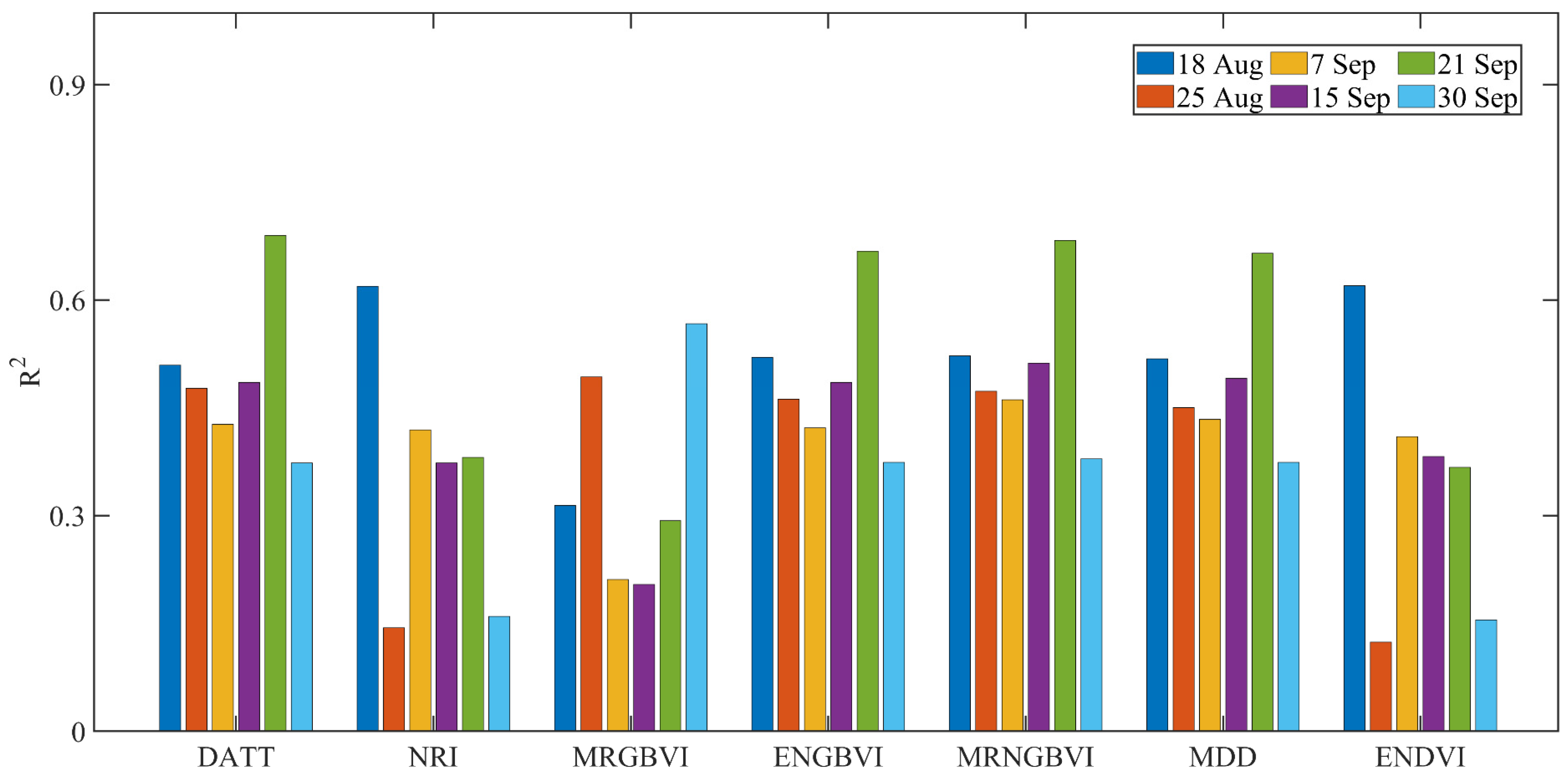
3.2. Linear Regression Analysis between Indices and SPAD Values

The linear regression analysis was performed between the VIs and SPAD values during the entire growing season. The regression equations with R², and p-values of the first ten indices were shown (

Table 4. The results of linear regression analysis between spectral indices and SPAD values of the entire growing season. The first column indicates the name of spectral indices, the second column is the linear regression equations, and the third and fourth columns are the R² and p, respectively.

Spectral Indices	Linear Regression Equations	R2	p
NDRE	Y = 31.07X + 62.76	0.412	p < 0.001
RECI	Y = 38.74X + 12.60	0.389	p < 0.001
ENDVI	Y = 59.29X − 14.00	0.352	p < 0.001
DATT	Y = 24.16X + 53.00	0.411	p < 0.001
NGI	Y = 90.11X − 127.24	0.332	p < 0.001
MCARI	Y = 42.40X + 30.29	0.381	p < 0.001
MRGBVI	Y = 60.76X – 14.77	0.328	p < 0.001
MRNRVI	Y = 30.01X + 9.92	0.376	p < 0.001
MTCI	Y = 39.96X + 9.74	0.375	p < 0.001
MDD	Y = 50.67X + 58.37	0.399	p < 0.001

). The R² ranged from 0.001 to 0.412 with p-values significant. Thus, the R² was not relatively high enough, and the top ten largest R² were shown with equations. The linear regression coefficients were different for different growing stages of maize and the modeling of SPAD values at each growth stages should rely on data collected on the same day.

The SIs and SPAD values at each growth stage of maize was conducted using the linear regression analysis, and the first seven indices with high R² are shown in Figure 6. The detailed results of the regression equations, R² and p-values of linear regression analysis, were given (

Table A2. The result of linear regression analysis between SIs and SPAD values for different growth stages. The spectral indices mean different information, and the stages are in according with the date of data acquisition in Figure 3. The Equation represents the linear regression equation, R² means the coefficient of determination, and the p means the significant values.

Spectral Indices	Stages	Equations	R2	p	Stages	Equations	R2	p
ENDVI	1	Y = −19.4X + 67.44	0.509	p <0.001	2	Y = −12.6X + 59.88	0.477	p < 0.001
	3	Y = −15.92X + 60.23	0.485	p < 0.001	4	Y = −12.44X + 59.36	0.427	p = 0.002
	5	Y = −24.88X + 62.32	0.690	p < 0.001	6	Y = −13.13X + 53.32	0.373	p = 0.004
DATT	1	Y = 42.23X + 31.65	0.144	p = 0.099	2	Y = 26.33X + 40.57	0.373	p = 0.002
	3	Y = 52.42X + 26.01	0.582	p = 0.004	4	Y = 55.61X + 21.48	0.381	p = 0.004
	5	Y = 75.03X + 11.66	0.160	p = 0.008	6	Y = 36.43X + 29.99	0.464	p < 0.001
NRI	1	Y = 404.58X + 40.71	0.314	p = 0.001	2	Y = 420.27X + 38.92	0.493	p < 0.001
	3	Y = −885.74X + 84.08	0.211	p = 0.042	4	Y = 517.44X + 34.17	0.204	p = 0.045
	5	Y = −1211.04X + 99.23	0.293	p = 0.014	6	Y = −131.92X + 104.61	0.567	p < 0.001
MRGBVI	1	Y = −24.85X + 72.75	0.520	p < 0.001	2	Y = −14.19X + 61.84	0.462	p < 0.001
	3	Y = −17.16X + 61.82	0.422	p < 0.001	4	Y = −13.3X + 60.47	0.485	p < 0.001
	5	Y = −27.72X + 65.87	0.668	p < 0.001	6	Y = −14.31X + 54.83	0.374	p = 0.004
ENGBVI	1	Y = −20.64X + 68.26	0.522	p < 0.001	2	Y = −12.37X + 59.44	0.473	p = 0.002
	3	Y = −15.12X + 58.24	0.461	p < 0.001	4	Y = −11.32X + 57.99	0.512	p < 0.001
	5	Y = −22.97X + 60.23	0.683	p < 0.001	6	Y = −11.03X + 51.37	0.379	p = 0.004
MRNGBVI	1	Y = −24.57X + 72.52	0.518	p < 0.001	2	Y = −13.62X + 61.54	0.450	p = 0.002
	3	Y = −17.24X + 61.71	0.434	p < 0.001	4	Y = −13.78X + 60.84	0.491	p < 0.001
	5	Y = −26.74X + 64.89	0.665	p < 0.001	6	Y = −13.52X + 54.04	0.374	p = 0.004
MDD	1	Y = 45.81X + 52.76	0.620	p < 0.001	2	Y = 26.79X + 53.91	0.124	p = 0.128
	3	Y = 56.37X + 52.43	0.410	p = 0.002	4	Y = 60.72X + 49.19	0.382	p = 0.004
	5	Y = 86.66X + 49.29	0.367	p = 0.005	6	Y = 45.13X + 48.22	0.155	p = 0.086

Note: 1–6 each represented different growth stages: 18 August (tasseling date), 25 August (silking), 7 September (blister), 15 September (milk), 21 September (physiological maturity), and 30 September (maturity).

). The average values of R² using the higher seven indices were 0.5174, 0.375, 0.398, 0.4189, 0.535, 0.512, and 0.340 for the different growth stages of maize. The R² using different growth stages were commonly larger than those using the entire growing season. The highest R² occurred on 21 September, indicating that the phenology was a very important indicator for predicting SPAD values.

The linear regression analysis was conducted between TIs and SPAD values at each growth stage of maize (Figure 7). The detailed results of R² and p values are given in

Table A3. The result of linear regression analysis between textural indices and SPAD values for different growth stages. The textural indices mean different textural information, and the stages are in according with the date of data acquisition in Figure 3. The Equation represents the linear regression equation, R² means the coefficient of determination, and the p means the significant values.

Textural Indices	Stages	Equations	R2	p	Stages	Equations	R2	p
Contrast	1	Y = 34.80X + 51.21	0.185	p < 0.001	2	Y = 45.12X + 48.23	0.478	p < 0.001
	3	Y = −42.39X + 61.80	0.151	p < 0.001	4	Y = 51.20X + 47.13	0.122	p < 0.001
	5	Y = 44.6X + 43.02	0.014	p < 0.001	6	Y = 50.76X + 35.01	0.381	p = 0.004
Correlation	1	Y = −50.46X + 84.27	0.255	p < 0.001	2	Y = −26.49X + 69.76	0.088	p = 0.002
	3	Y = −56.10X + 81.05	0.358	p < 0.001	4	Y = −23.57X + 67.19	0.147	p < 0.001
	5	Y = −102.57X + 103.22	0.545	p < 0.001	6	Y = −1.95X + 48.92	0.228	p = 0.004
Energy	1	Y = −9.83X + 61.59	0.129	p < 0.001	2	Y = −17.87X + 65.01	0.511	p = 0.002
	3	Y = 38.99X + 33.21	0.284	p < 0.001	4	Y = −17.77X + 64.48	0.116	p < 0.001
	5	Y = 68.31X + 23.33	0.289	p < 0.001	6	Y = −29.41X + 58.77	0.566	p = 0.004
Homogeneity	1	Y = −69.60X + 120.81	0.185	p < 0.001	2	Y = −90.25X + 138.49	0.478	p = 0.128
	3	Y = 84.79X − 22.98	0.051	p = 0.002	4	Y = −102.40X + 149.54	0.122	p = 0.004
	5	Y = −89.32X + 132.35	0.014	p = 0.005	6	Y = −101.52X + 136.53	0.381	p = 0.086

Note: 1–6 each represented different growth stages: 18 August (tasseling date), 25 August (silking), 7 September (blister), 15 September (milk), 21 September (physiological maturity), and 30 September (maturity).

. The average values of R² using the TIs were 0.189, 0.389, 0.211, 0.127, 0.216, and 0.389, respectively. It can be indicated that the R² using TIs were also different for different growth stages of maize, and the highest R² occurred on 25 August.

The results of SRM for identifying the optimal combination of SIs and TIs for predicting SPAD values at each growth stage of maize are shown in

Table 5. The optimal combinations of spectral and textural indices for predicting SPAD values using stepwise regression model. The first column represents the different dates of data acquisition, the second column is the corresponding phenology, and the third and fourth columns are the optimized combinations of spectral and textural indices.

Dates	Phenology	Spectral Indices	Textural Indices
18 August	tasseling date	ENDVI, DATT, NRI, MRGBVI, ENGBVI, MRNGBVI	Contrast, Correlation, Energy, Homogeneity
25 August	silking	ENDVI, DATT, NRI, MRGBVI, ENGBVI, MRNGBVI	Contrast, Correlation, Homogeneity
7 September	blister	ENDVI, NRI, MRGBVI, MRNGBVI, MDD	Contrast, Correlation, Energy, Homogeneity
15 September	milk	ENDVI, NRI, MRGBVI, ENGBVI, MRNGBVI	Contrast, Correlation, Energy, Homogeneity
21 September	physiological maturity	ENDVI, NRI, MRGBVI, ENGBVI, MRNGBVI, MDD	Contrast, Energy, Homogeneity
30 September	maturity	ENDVI, NRI, MRGBVI, ENGBVI, MRNGBVI, MDD	Contrast, Energy, Homogeneity

.

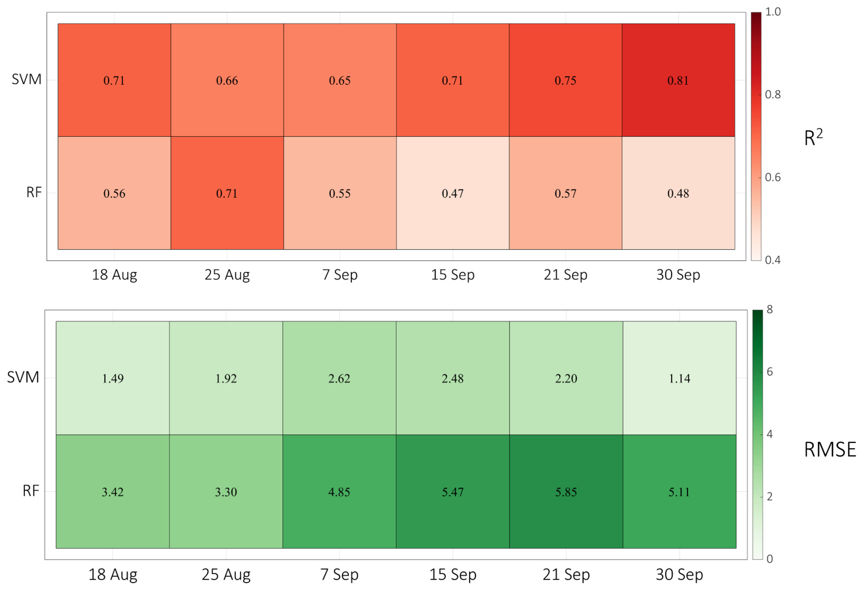
3.3. Predicting SPAD Values of Maize Using Machine Learning Methods

RF and SVM models were independently built for predicting SPAD values, and the results of evaluations are shown in Figure 8. It can be easily observed that R² of SVM were commonly larger than RF, and similarly, the RMSEs of SVM were commonly smaller than RF. Thus, SVM performed better than RF, and SVM may have greater potential ability in predicting SPAD values of maize at different growth stage.

The parameters with highest R² and lowest RMSE of RF and SVM were applied for predicting SPAD values at different growth stages of maize (Figure 9 and Figure 10). It should be noted that there was a significant difference between the predicted SPAD values using RF and SVM.

4. Discussion

4.1. The Radiometric Calibration of the Multi-Spectral Images Using ELCM

In this study, the radiometric calibration of MMC was performed using ELCM. The critical innovation laid in the general equations for radiometric calibration were confirmed using data collected from multi-days (sunny and cloudless). Thus, the calibrated reflectance will be more precise and more reliable by reducing accidental errors, atmospheric effects, and dark noise. The R² of the calibration were 0.874 and 0.927, and the RMSE (NRMSE) were 0.110 (0.177) and 0.089 (0.138), using data collected on 5 August and 21 September, respectively. The R² (0.883) and RMSE (5.6%) for the radiometric calibration of MMC were reported [29]. It was reported the ELCM was applied for the radiometric calibration of MMC and RMSE ranged from 0.025 to 0.064% [30]. The maximum error means of six bands were tested and confirmed as 8% [31]. Similar results were also obtained in the radiometric calibration for ultra-high-resolution of five bands multi-spectral images acquired from the UAV system, where the RMSE was 0.063% for calibration targets and 0.040, 0.048, and 0.089% for the red, green, and blue bands, respectively [103]. The R² for red and NIR bands ranged from 0.96 to 0.99, and from 0.95 to 0.99 with five different calibration targets using ELCM, respectively [104]. There should also be noted that the calibration and validation were based on the data collected in a single day in most previous studies. However, as introduced in the section method the calibration in this study was based on data collected on six different phenological dates, and the validation was conducted by comparing the reflectance of maize on 5 August and 21 September. Therefore, the radiometric calibration of this study was more convincing concerning the results from previous studies. Despite the relatively high accuracy, there still remained uncertainties to be addressed. Firstly, the synchronous reflectance measurement of the calibration targets was difficult to perform as the weather conditions changed rapidly during the data collection. Secondly, the precise locations of maize for validation on 5 August and 21 September were difficult to confirm in images due to the coarse spatial resolution of the multi-spectral images (5 cm). Moreover, the sampled reflectance of maize was influenced by mixed pixels (soil and maize). Thirdly, the Bidirectional reflectance distribution function (BRDF) that can influence the reflectance of the calibration target was ignored [105]. The BRDF is defined as reflectivity in different reflection directions, and thus, for the ground objects such as maize there was an optimal observation angle to obtain the highest accuracy. The important biophysical structural parameters, such as vegetation structure and vegetation cover fraction, can be derived from BRDF. However, the application of BRDF was based on the images collected from different angles. This was highly difficult to perform during the whole growth stage period of maize. Therefore, the BRDF was not explored in the current study, and future studies could include such issues for obtaining more reliable results.

4.2. The Predictions of the SPAD Values of Maize

In previous studies, the vegetation indices, such as NDVI and enhanced vegetation index (EVI), were mainly applied to monitor crops’ growth conditions. Commonly, the spectral indices were directly applied to predict SPAD values using linear or non-linear regression models. However, the mechanisms for different growth stage may be different, as the spectral indices varied dramatically at different growth stages of maize. In this study, the optimal combination of SIs and TIs were separately confirmed using SRM. The TIs were closely correlated with SPAD values compared with the SIs. The TIs have great potentials in predicting SPAD values, and this was in consistence with previous studies where the integrated SIs and TIs achieved high accuracy in expressing the dynamic growth condition of maize at different growth stages [10,106]. Although relatively high accuracy was achieved, there were still limitations in predicting SPAD values. Firstly, the sampled SPAD values using SPAD-502Plus may not be so representative for each plot. Thus, more samples can be included for minimizing the uncertainties in future analysis. Secondly, the Sis and Tis calculated may be influenced by mixed pixels. Methods for extracting pixels only containing maize should be proposed. Thirdly, the SPAD can be converted into physiological parameters, such as leaf chlorophyll content, which is commonly applied to assess the leaf photosynthetic capacity and leaf nitrogen content. However, in the current study, the precise measurement of leaf chlorophyll content was not performed, and thus, the linear regressions between the SPAD values and leaf chlorophyll content can hardly be obtained. Therefore, it was recommended the adoption of leaf chlorophyll content for monitoring the growth condition and yield prediction of maize in future analysis.

SVM and RF were independently applied to predict SPAD values. In Figure 9, the accuracy of SVM were usually higher than that using RF. There was a significant improvement in R² and RMSE by SVM compared with RF. SVM is a novel small sample learning method with a solid theoretical foundation. In essence, it can avoid the traditional process from induction to deduction, realizing the efficient “transduction reasoning” from training samples to prediction samples, simplifying the usual problems such as classification and regression [107,108]. SVM has realized good “robustness” compared with other machine learning methods, as the adding and deleting non-supporting vector samples had no effects to the original model [109]. SVM could perform well with little data, which was quite useful when the number of samples was limited. Even though SVM achieved relatively high accuracy with limited samples of SPAD values, and it was still recommended the conduction of more ground samples. Moreover, SVM and RF models were relatively traditional ones, and there is need to evaluate more advanced models for predicting SPAD values in future analysis.

5. Conclusions

In this study, the empirical line calibration method was applied for obtaining the generic equations based on the multi-spectral images on multiple days, and results showed the radiometric calibration achieved high accuracy. The commonly applied spectral and textural indices were extracted from multi-spectral images, and the linear regression analysis was conducted between these indices and SPAD values. Both spectral and textural indices were closely correlated with the SPAD values. The stepwise regression model was applied to select the optimal combination of spectral and textural indices for predicting SPAD values at different growth stages. The results showed the proposed method by combing spectral and textural indices improved the estimation accuracy. Precisely estimating SPAD values offers potential for obtaining leaf chlorophyll content, which is a very important indicator of chloroplast development, photosynthetic capacity, and leaf nitrogen content for monitoring plant health. The SPAD values can be converted into leaf nitrogen content for better retrieving the physiological parameters of maize. SVM and RF were independently conducted to predict SPAD values based on optimal combinations. The results showed that SVM performed better than RF with higher R² and lower RMSE. Therefore, it is highly recommended the adoption of optimal combination of spectral and textural indices for estimating SPAD values of maize using SVM.

References

1. Guo, Y.; Yin, G.; Sun, H.; Wang, H.; Chen, S.; Senthilnath, J.; Wang, J.; Fu, Y. Scaling effects on chlorophyll content estimations with RGB camera mounted on a UAV platform using machine-learning methods. Sensors 2020, 20, 5130. [Google Scholar] [CrossRef] [PubMed]
2. Li, S.; Yuan, F.; Ata-UI-Karim, S.T.; Zheng, H.; Cheng, T.; Liu, X.; Tian, Y.; Zhu, Y.; Cao, W.; Cao, Q. Combining color indices and textures of UAV-based digital imagery for rice LAI estimation. Remote Sens. 2019, 11, 1763. [Google Scholar] [CrossRef] [Green Version]
3. Li, X.; Li, X.; Liu, W.; Wei, B.; Xu, X. A UAV-based framework for crop lodging assessment. Eur. J. Agron. 2021, 123, 126201. [Google Scholar] [CrossRef]
4. Nowak, M.M.; Dziób, K.; Bogawski, P. Unmanned Aerial Vehicles (UAVs) in environmental biology: A review. Eur. J. Ecol. 2018, 4, 56–74. [Google Scholar] [CrossRef]
5. Aasen, H.; Burkart, A.; Bolten, A.; Bareth, G. Generating 3D hyperspectral information with lightweight UAV snapshot cameras for vegetation monitoring: From camera calibration to quality assurance. ISPRS J. Photogramm. Remote Sens. 2015, 108, 245–259. [Google Scholar] [CrossRef]
6. Alsalam, B.H.Y.; Morton, K.; Campbell, D.; Gonzalez, F. Autonomous UAV with vision based on-board decision making for remote sensing and precision agriculture. In Proceedings of the 2017 IEEE Aerospace Conference, Big Sky, MT, USA, 4–11 March 2017; pp. 1–12. [Google Scholar]
7. Xiang, H.; Tian, L. Development of a low-cost agricultural remote sensing system based on an autonomous unmanned aerial vehicle (UAV). Biosyst. Eng. 2011, 108, 174–190. [Google Scholar] [CrossRef]
8. Vickers, N.J. Animal communication: When i’m calling you, will you answer too? Curr. Biol. 2017, 27, R713–R715. [Google Scholar] [CrossRef]
9. Fu, Y.; Yang, G.; Song, X.; Li, Z.; Xu, X.; Feng, H.; Zhao, C. Improved estimation of winter wheat aboveground biomass using multiscale textures extracted from UAV-based digital images and hyperspectral feature analysis. Remote Sens. 2021, 13, 581. [Google Scholar] [CrossRef]
10. Guo, Y.; Chen, S.; Wu, Z.; Wang, S.; Robin Bryant, C.; Senthilnath, J.; Cunha, M.; Fu, Y.H. Integrating Spectral and Textural Information for Monitoring the Growth of Pear Trees Using Optical Images from the UAV Platform. Remote Sens. 2021, 13, 1795. [Google Scholar] [CrossRef]
11. Guo, Y.; Wang, H.; Wu, Z.; Wang, S.; Sun, H.; Senthilnath, J.; Wang, J.; Robin Bryant, C.; Fu, Y. Modified red blue vegetation index for chlorophyll estimation and yield prediction of maize from visible images captured by UAV. Sensors 2020, 20, 5055. [Google Scholar] [CrossRef]
12. Kestur, R.; Angural, A.; Bashir, B.; Omkar, S.; Anand, G.; Meenavathi, M. Tree crown detection, delineation and counting in uav remote sensed images: A neural network based spectral–spatial method. J. Indian Soc. Remote Sens. 2018, 46, 991–1004. [Google Scholar] [CrossRef]
13. Senthilnath, J.; Dokania, A.; Kandukuri, M.; Ramesh, K.; Anand, G.; Omkar, S. Detection of tomatoes using spectral-spatial methods in remotely sensed RGB images captured by UAV. Biosyst. Eng. 2016, 146, 16–32. [Google Scholar] [CrossRef]
14. Ammoniaci, M.; Kartsiotis, S.-P.; Perria, R.; Storchi, P. State of the Art of Monitoring Technologies and Data Processing for Precision Viticulture. Agriculture 2021, 11, 201. [Google Scholar] [CrossRef]
15. Pallottino, F.; Figorilli, S.; Cecchini, C.; Costa, C. Light Drones for Basic In-Field Phenotyping and Precision Farming Applications: RGB Tools Based on Image Analysis. In Crop Breeding; Springer: New York, NY, USA, 2021; pp. 269–278. [Google Scholar]
16. Yang, G.; Liu, J.; Zhao, C.; Li, Z.; Huang, Y.; Yu, H.; Xu, B.; Yang, X.; Zhu, D.; Zhang, X. Unmanned aerial vehicle remote sensing for field-based crop phenotyping: Current status and perspectives. Front. Plant Sci. 2017, 8, 1111. [Google Scholar] [CrossRef]
17. Lang, Q.; Zhiyong, Z.; Longsheng, C.; Hong, S.; Minzan, L.; Li, L.; Junyong, M. Detection of chlorophyll content in Maize Canopy from UAV Imagery. IFAC Pap. 2019, 52, 330–335. [Google Scholar] [CrossRef]
18. Damayanti, R.; Nainggolan, R.; Al Riza, D.; Hendrawan, Y. Application of RGB-CCM and GLCM texture analysis to predict chlorophyll content in Vernonia amygdalina. In Proceedings of the Fourth International Seminar on Photonics, Optics, and Its Applications (ISPhOA 2020), Sanur, Indonesia, 12 March 2021; p. 1178907. [Google Scholar]
19. Adão, T.; Hruška, J.; Pádua, L.; Bessa, J.; Peres, E.; Morais, R.; Sousa, J.J. Hyperspectral imaging: A review on UAV-based sensors, data processing and applications for agriculture and forestry. Remote Sens. 2017, 9, 1110. [Google Scholar] [CrossRef] [Green Version]
20. Gago, J.; Douthe, C.; Coopman, R.E.; Gallego, P.P.; Ribas-Carbo, M.; Flexas, J.; Escalona, J.; Medrano, H. UAVs challenge to assess water stress for sustainable agriculture. Agric. Water Manag. 2015, 153, 9–19. [Google Scholar] [CrossRef]
21. Senthilnath, J.; Kumar, A.; Jain, A.; Harikumar, K.; Thapa, M.; Suresh, S.; Anand, G.; Benediktsson, J.A. BS-McL: Bilevel Segmentation Framework with Metacognitive Learning for Detection of the Power Lines in UAV Imagery. IEEE Trans. Geosci. Remote Sens. 2021, 60, 1–12. [Google Scholar] [CrossRef]
22. Guo, Y.; Fu, Y.H.; Chen, S.; Bryant, C.R.; Li, X.; Senthilnath, J.; Sun, H.; Wang, S.; Wu, Z.; de Beurs, K. Integrating spectral and textural information for identifying the tasseling date of summer maize using UAV based RGB images. Int. J. Appl. Earth Obs. Geoinf. 2021, 102, 102435. [Google Scholar] [CrossRef]
23. Guo, Y.; Senthilnath, J.; Wu, W.; Zhang, X.; Zeng, Z.; Huang, H. Radiometric calibration for multispectral camera of different imaging conditions mounted on a UAV platform. Sustainability 2019, 11, 978. [Google Scholar] [CrossRef] [Green Version]
24. Turner, D.; Lucieer, A.; Malenovský, Z.; King, D.H.; Robinson, S.A. Spatial co-registration of ultra-high resolution visible, multispectral and thermal images acquired with a micro-UAV over Antarctic moss beds. Remote Sens. 2014, 6, 4003–4024. [Google Scholar] [CrossRef] [Green Version]
25. Guanter, L.; Zhang, Y.; Jung, M.; Joiner, J.; Voigt, M.; Berry, J.A.; Frankenberg, C.; Huete, A.R.; Zarco-Tejada, P.; Lee, J.-E. Global and time-resolved monitoring of crop photosynthesis with chlorophyll fluorescence. Proc. Natl. Acad. Sci. USA 2014, 111, E1327–E1333. [Google Scholar] [CrossRef] [PubMed] [Green Version]
26. Ghrefat, H.A.; Goodell, P.C. Land cover mapping at Alkali Flat and Lake Lucero, White Sands, New Mexico, USA using multi-temporal and multi-spectral remote sensing data. Int. J. Appl. Earth Obs. Geoinf. 2011, 13, 616–625. [Google Scholar] [CrossRef]
27. Yubin, L.; Xiaoling, D.; Guoliang, Z. Advances in diagnosis of crop diseases, pests and weeds by UAV remote sensing. Smart Agric. 2019, 1, 1. [Google Scholar]
28. Wang, C.; Myint, S.W. A simplified empirical line method of radiometric calibration for small unmanned aircraft systems-based remote sensing. IEEE J. Sel. Top. Appl. Earth Obs. Remote Sens. 2015, 8, 1876–1885. [Google Scholar] [CrossRef]
29. Laliberte, A.S.; Goforth, M.A.; Steele, C.M.; Rango, A. Multispectral remote sensing from unmanned aircraft: Image processing workflows and applications for rangeland environments. Remote Sens. 2011, 3, 2529–2551. [Google Scholar] [CrossRef] [Green Version]
30. Iqbal, F.; Lucieer, A.; Barry, K. Simplified radiometric calibration for UAS-mounted multispectral sensor. Eur. J. Remote Sens. 2018, 51, 301–313. [Google Scholar] [CrossRef]
31. Del Pozo, S.; Rodríguez-Gonzálvez, P.; Hernández-López, D.; Felipe-García, B. Vicarious radiometric calibration of a multispectral camera on board an unmanned aerial system. Remote Sens. 2014, 6, 1918–1937. [Google Scholar] [CrossRef] [Green Version]
32. Badgley, G.; Anderegg, L.D.; Berry, J.A.; Field, C.B. Terrestrial gross primary production: Using NIRV to scale from site to globe. Glob. Change Biol. 2019, 25, 3731–3740. [Google Scholar] [CrossRef]
33. Robinson, N.P.; Allred, B.W.; Jones, M.O.; Moreno, A.; Kimball, J.S.; Naugle, D.E.; Erickson, T.A.; Richardson, A.D. A dynamic Landsat derived normalized difference vegetation index (NDVI) product for the conterminous United States. Remote Sens. 2017, 9, 863. [Google Scholar] [CrossRef] [Green Version]
34. Wu, C.; Niu, Z.; Tang, Q.; Huang, W.; Rivard, B.; Feng, J. Remote estimation of gross primary production in wheat using chlorophyll-related vegetation indices. Agric. For. Meteorol. 2009, 149, 1015–1021. [Google Scholar] [CrossRef]
35. Chen, P.; Feng, H.; Li, C.; Yang, G.; Yang, J.; Yang, W.; Liu, S. Estimation of chlorophyll content in potato using fusion of texture and spectral features derived from UAV multispectral image. Trans. Chin. Soc. Agric. Eng. 2019, 35, 63–74. [Google Scholar]
36. Bhatta, B. Analysis of urban growth pattern using remote sensing and GIS: A case study of Kolkata, India. Int. J. Remote Sens. 2009, 30, 4733–4746. [Google Scholar] [CrossRef]
37. Franch, B.; Vermote, E.F.; Skakun, S.; Roger, J.-C.; Becker-Reshef, I.; Murphy, E.; Justice, C. Remote sensing based yield monitoring: Application to winter wheat in United States and Ukraine. Int. J. Appl. Earth Obs. Geoinf. 2019, 76, 112–127. [Google Scholar] [CrossRef]
38. Sahurkar, S.; Chilke, B. Assessment of chlorophyll and nitrogen contents of leaves using image processing technique. Int. Res. J. Eng. Technol. 2017, 4, 2243–2247. [Google Scholar]
39. Hussain, M.; Chen, D.; Cheng, A.; Wei, H.; Stanley, D. Change detection from remotely sensed images: From pixel-based to object-based approaches. ISPRS J. Photogramm. Remote Sens. 2013, 80, 91–106. [Google Scholar] [CrossRef]
40. Shackelford, A.K.; Davis, C.H. A combined fuzzy pixel-based and object-based approach for classification of high-resolution multispectral data over urban areas. IEEE Trans. Geosci. Remote Sens. 2003, 41, 2354–2363. [Google Scholar] [CrossRef] [Green Version]
41. Yang, K.; Gong, Y.; Fang, S.; Duan, B.; Yuan, N.; Peng, Y.; Wu, X.; Zhu, R. Combining spectral and texture features of UAV images for the remote estimation of rice LAI throughout the entire growing season. Remote Sens. 2021, 13, 3001. [Google Scholar] [CrossRef]
42. Peña-Barragán, J.M.; Ngugi, M.K.; Plant, R.E.; Six, J. Object-based crop identification using multiple vegetation indices, textural features and crop phenology. Remote Sens. Environ. 2011, 115, 1301–1316. [Google Scholar] [CrossRef]
43. Shah, S.H.; Houborg, R.; McCabe, M.F. Response of chlorophyll, carotenoid and SPAD-502 measurement to salinity and nutrient stress in wheat (Triticum aestivum L.). Agronomy 2017, 7, 61. [Google Scholar] [CrossRef] [Green Version]
44. Hawkins, T.S.; Gardiner, E.S.; Comer, G.S. Modeling the relationship between extractable chlorophyll and SPAD-502 readings for endangered plant species research. J. Nat. Conserv. 2009, 17, 123–127. [Google Scholar] [CrossRef]
45. Loh, F.C.; Grabosky, J.C.; Bassuk, N.L. Using the SPAD 502 meter to assess chlorophyll and nitrogen content of benjamin fig and cottonwood leaves. HortTechnology 2002, 12, 682–686. [Google Scholar] [CrossRef] [Green Version]
46. Coste, S.; Baraloto, C.; Leroy, C.; Marcon, É.; Renaud, A.; Richardson, A.D.; Roggy, J.-C.; Schimann, H.; Uddling, J.; Hérault, B. Assessing foliar chlorophyll contents with the SPAD-502 chlorophyll meter: A calibration test with thirteen tree species of tropical rainforest in French Guiana. Ann. For. Sci. 2010, 67, 607. [Google Scholar] [CrossRef] [Green Version]
47. Zhang, S.; Zhao, G.; Lang, K.; Su, B.; Chen, X.; Xi, X.; Zhang, H. Integrated satellite, unmanned aerial vehicle (UAV) and ground inversion of the SPAD of winter wheat in the reviving stage. Sensors 2019, 19, 1485. [Google Scholar] [CrossRef] [Green Version]
48. Duan, B.; Fang, S.; Zhu, R.; Wu, X.; Wang, S.; Gong, Y.; Peng, Y. Remote estimation of rice yield with unmanned aerial vehicle (UAV) data and spectral mixture analysis. Front. Plant Sci. 2019, 10, 204. [Google Scholar] [CrossRef] [Green Version]
49. Shu, M.; Zuo, J.; Shen, M.; Yin, P.; Wang, M.; Yang, X.; Tang, J.; Li, B.; Ma, Y. Improving the estimation accuracy of SPAD values for maize leaves by removing UAV hyperspectral image backgrounds. Int. J. Remote Sens. 2021, 42, 5862–5881. [Google Scholar] [CrossRef]
50. Yang, X.; Yang, R.; Ye, Y.; Yuan, Z.; Wang, D.; Hua, K. Winter wheat SPAD estimation from UAV hyperspectral data using cluster-regression methods. Int. J. Appl. Earth Obs. Geoinf. 2021, 105, 102618. [Google Scholar] [CrossRef]
51. Liu, Y.; Hatou, K.; Aihara, T.; Kurose, S.; Akiyama, T.; Kohno, Y.; Lu, S.; Omasa, K. A robust vegetation index based on different UAV RGB images to estimate SPAD values of naked barley leaves. Remote Sens. 2021, 13, 686. [Google Scholar] [CrossRef]
52. Wan, L.; Cen, H.; Zhu, J.; Zhang, J.; Zhu, Y.; Sun, D.; Du, X.; Zhai, L.; Weng, H.; Li, Y. Grain yield prediction of rice using multi-temporal UAV-based RGB and multispectral images and model transfer–A case study of small farmlands in the South of China. Agric. For. Meteorol. 2020, 291, 108096. [Google Scholar] [CrossRef]
53. Shendryk, Y.; Sofonia, J.; Garrard, R.; Rist, Y.; Skocaj, D.; Thorburn, P. Fine-scale prediction of biomass and leaf nitrogen content in sugarcane using UAV LiDAR and multispectral imaging. Int. J. Appl. Earth Obs. Geoinf. 2020, 92, 102177. [Google Scholar] [CrossRef]
54. Meng, R.; Lv, Z.; Yan, J.; Chen, G.; Zhao, F.; Zeng, L.; Xu, B. Development of Spectral Disease Indices for Southern Corn Rust Detection and Severity Classification. Remote Sens. 2020, 12, 3233. [Google Scholar] [CrossRef]
55. Berni, J.A.; Zarco-Tejada, P.J.; Suárez, L.; Fereres, E. Thermal and narrowband multispectral remote sensing for vegetation monitoring from an unmanned aerial vehicle. IEEE Trans. Geosci. Remote Sens. 2009, 47, 722–738. [Google Scholar] [CrossRef] [Green Version]
56. Stagakis, S.; González-Dugo, V.; Cid, P.; Guillén-Climent, M.L.; Zarco-Tejada, P.J. Monitoring water stress and fruit quality in an orange orchard under regulated deficit irrigation using narrow-band structural and physiological remote sensing indices. ISPRS J. Photogramm. Remote Sens. 2012, 71, 47–61. [Google Scholar] [CrossRef] [Green Version]
57. Deng, L.; Mao, Z.; Li, X.; Hu, Z.; Duan, F.; Yan, Y. UAV-based multispectral remote sensing for precision agriculture: A comparison between different cameras. ISPRS J. Photogramm. Remote Sens. 2018, 146, 124–136. [Google Scholar] [CrossRef]
58. Canty, M.J. Image Analysis, Classification and Change Detection in Remote Sensing: With Algorithms for ENVI/IDL and Python; CRC Press: Boca Raton, FL, USA, 2014. [Google Scholar]
59. Salata, F.; Golasi, I.; de Lieto Vollaro, R.; de Lieto Vollaro, A. Urban microclimate and outdoor thermal comfort. A proper procedure to fit ENVI-met simulation outputs to experimental data. Sustain. Cities Soc. 2016, 26, 318–343. [Google Scholar] [CrossRef]
60. Hassan, M.A.; Yang, M.; Rasheed, A.; Jin, X.; Xia, X.; Xiao, Y.; He, Z. Time-series multispectral indices from unmanned aerial vehicle imagery reveal senescence rate in bread wheat. Remote Sens. 2018, 10, 809. [Google Scholar] [CrossRef] [Green Version]
61. Oniga, V.-E.; Breaban, A.-I.; Statescu, F. Determining the optimum number of ground control points for obtaining high precision results based on UAS images. In Proceedings of the Multidisciplinary Digital Publishing Institute Proceedings, online conference, 22 March–5 April 2018; p. 352. [Google Scholar]
62. Chen, W.; Yan, L.; Li, Z.; Jing, X.; Duan, Y.; Xiong, X. In-flight absolute calibration of an airborne wide-view multispectral imager using a reflectance-based method and its validation. Int. J. Remote Sens. 2013, 34, 1995–2005. [Google Scholar] [CrossRef]
63. Bielinis, E.; Jozwiak, W.; Robakowski, P. Modelling of the relationship between the SPAD values and photosynthetic pigments content in Quercus petraea and Prunus serotina leaves. Dendrobiology 2015, 73, 125–134. [Google Scholar] [CrossRef] [Green Version]
64. Kumar, P.; Sharma, R. Development of SPAD value-based linear models for non-destructive estimation of photosynthetic pigments in wheat (Triticum aestivum L.). Indian J. Genet. 2019, 79, 96–99. [Google Scholar] [CrossRef]
65. Smith, G.M.; Milton, E.J. The use of the empirical line method to calibrate remotely sensed data to reflectance. Int. J. Remote Sens. 1999, 20, 2653–2662. [Google Scholar] [CrossRef]
66. Tucker, C.J. Red and photographic infrared linear combinations for monitoring vegetation. Remote Sens. Environ. 1979, 8, 127–150. [Google Scholar] [CrossRef] [Green Version]
67. Zheng, H.; Cheng, T.; Li, D.; Zhou, X.; Yao, X.; Tian, Y.; Cao, W.; Zhu, Y. Evaluation of RGB, color-infrared and multispectral images acquired from unmanned aerial systems for the estimation of nitrogen accumulation in rice. Remote Sens. 2018, 10, 824. [Google Scholar] [CrossRef] [Green Version]
68. Brovkina, O.; Cienciala, E.; Surový, P.; Janata, P. Unmanned aerial vehicles (UAV) for assessment of qualitative classification of Norway spruce in temperate forest stands. Geo-Spat. Inf. Sci. 2018, 21, 12–20. [Google Scholar] [CrossRef] [Green Version]
69. Huang, W.; Yang, Q.; Pu, R.; Yang, S. Estimation of nitrogen vertical distribution by bi-directional canopy reflectance in winter wheat. Sensors 2014, 14, 20347–20359. [Google Scholar] [CrossRef] [PubMed] [Green Version]
70. Tahir, M.N.; Naqvi, S.Z.A.; Lan, Y.; Zhang, Y.; Wang, Y.; Afzal, M.; Cheema, M.J.M.; Amir, S. Real time estimation of chlorophyll content based on vegetation indices derived from multispectral UAV in the kinnow orchard. Int. J. Precis. Agric. Aviat. 2018, 1. [Google Scholar]
71. Dash, J.; Curran, P. Evaluation of the MERIS terrestrial chlorophyll index (MTCI). Adv. Space Res. 2007, 39, 100–104. [Google Scholar] [CrossRef]
72. Dash, J.; Curran, P.J.; Tallis, M.J.; Llewellyn, G.M.; Taylor, G.; Snoeij, P. Validating the MERIS Terrestrial Chlorophyll Index (MTCI) with ground chlorophyll content data at MERIS spatial resolution. Int. J. Remote Sens. 2010, 31, 5513–5532. [Google Scholar] [CrossRef] [Green Version]
73. Cao, Q.; Miao, Y.; Feng, G.; Gao, X.; Li, F.; Liu, B.; Yue, S.; Cheng, S.; Ustin, S.L.; Khosla, R. Active canopy sensing of winter wheat nitrogen status: An evaluation of two sensor systems. Comput. Electron. Agric. 2015, 112, 54–67. [Google Scholar] [CrossRef]
74. Duque, A.; Vázquez, C. Double attention bias for positive and negative emotional faces in clinical depression: Evidence from an eye-tracking study. J. Behav. Ther. Exp. Psychiatry 2015, 46, 107–114. [Google Scholar] [CrossRef]
75. Gitelson, A.; Merzlyak, M.N. Quantitative estimation of chlorophyll-a using reflectance spectra: Experiments with autumn chestnut and maple leaves. J. Photochem. Photobiol. B Biol. 1994, 22, 247–252. [Google Scholar] [CrossRef]
76. Virnodkar, S.S.; Pachghare, V.K.; Patil, V.C.; Jha, S.K. Remote sensing and machine learning for crop water stress determination in various crops: A critical review. Precis. Agric. 2020, 21, 1121–1155. [Google Scholar] [CrossRef]
77. Datt, B. Visible/near infrared reflectance and chlorophyll content in Eucalyptus leaves. Int. J. Remote Sens. 1999, 20, 2741–2759. [Google Scholar] [CrossRef]
78. Cao, Q.; Miao, Y.; Wang, H.; Huang, S.; Cheng, S.; Khosla, R.; Jiang, R. Non-destructive estimation of rice plant nitrogen status with Crop Circle multispectral active canopy sensor. Field Crops Res. 2013, 154, 133–144. [Google Scholar] [CrossRef]
79. Xiao, Y.; Zhao, W.; Zhou, D.; Gong, H. Sensitivity analysis of vegetation reflectance to biochemical and biophysical variables at leaf, canopy, and regional scales. IEEE Trans. Geosci. Remote Sens. 2013, 52, 4014–4024. [Google Scholar] [CrossRef]
80. Dall’Olmo, G.; Gitelson, A.A.; Rundquist, D.C.; Leavitt, B.; Barrow, T.; Holz, J.C. Assessing the potential of SeaWiFS and MODIS for estimating chlorophyll concentration in turbid productive waters using red and near-infrared bands. Remote Sens. Environ. 2005, 96, 176–187. [Google Scholar] [CrossRef]
81. Ferwerda, J.G.; Skidmore, A.K.; Mutanga, O. Nitrogen detection with hyperspectral normalized ratio indices across multiple plant species. Int. J. Remote Sens. 2005, 26, 4083–4095. [Google Scholar] [CrossRef]
82. Law, B.E.; Waring, R.H. Remote sensing of leaf area index and radiation intercepted by understory vegetation. Ecol. Appl. 1994, 4, 272–279. [Google Scholar] [CrossRef]
83. Shen, Z.; Fu, G.; Yu, C.; Sun, W.; Zhang, X. Relationship between the growing season maximum enhanced vegetation index and climatic factors on the Tibetan Plateau. Remote Sens. 2014, 6, 6765–6789. [Google Scholar] [CrossRef] [Green Version]
84. Peñuelas, J.; Gamon, J.; Fredeen, A.; Merino, J.; Field, C. Reflectance indices associated with physiological changes in nitrogen-and water-limited sunflower leaves. Remote Sens. Environ. 1994, 48, 135–146. [Google Scholar] [CrossRef]
85. Filella, I.; Serrano, L.; Serra, J.; Penuelas, J. Evaluating wheat nitrogen status with canopy reflectance indices and discriminant analysis. Crop Sci. 1995, 35, 1400–1405. [Google Scholar] [CrossRef]
86. Penuelas, J.; Gamon, J.A.; Griffin, K.L.; Field, C.B. Assessing community type, plant biomass, pigment composition, and photosynthetic efficiency of aquatic vegetation from spectral reflectance. Remote Sens. Environ. 1993, 46, 110–118. [Google Scholar] [CrossRef]
87. Wang, F.; Yi, Q.; Hu, J.; Xie, L.; Yao, X.; Xu, T.; Zheng, J. Combining spectral and textural information in UAV hyperspectral images to estimate rice grain yield. Int. J. Appl. Earth Obs. Geoinf. 2021, 102, 102397. [Google Scholar] [CrossRef]
88. Haralick, R.M.; Shanmugam, K.; Dinstein, I. Textural Features for Image Classification. Stud. Media Commun. 1973, SMC-3, 610–621. [Google Scholar] [CrossRef] [Green Version]
89. Thompson, B. Stepwise regression and stepwise discriminant analysis need not apply here: A guidelines editorial. Educ. Psychol. Measur. 1995, 55, 525–534. [Google Scholar] [CrossRef]
90. Bendel, R.B.; Afifi, A.A. Comparison of stopping rules in forward “stepwise” regression. J. Am. Stat. Assoc. 1977, 72, 46–53. [Google Scholar]
91. Liu, B.; Zhao, Q.; Jin, Y.; Shen, J.; Li, C. Application of combined model of stepwise regression analysis and artificial neural network in data calibration of miniature air quality detector. Sci. Rep. 2021, 11, 1–12. [Google Scholar] [CrossRef]
92. Jin, X.-L.; Wang, K.-R.; Xiao, C.-H.; Diao, W.-Y.; Wang, F.-Y.; Chen, B.; Li, S.-K. Comparison of two methods for estimation of leaf total chlorophyll content using remote sensing in wheat. Field Crops Res. 2012, 135, 24–29. [Google Scholar] [CrossRef]
93. Maulik, U.; Chakraborty, D. Remote Sensing Image Classification: A survey of support-vector-machine-based advanced techniques. IEEE Geosci. Remote Sens. Mag. 2017, 5, 33–52. [Google Scholar] [CrossRef]
94. Wang, M.; Wan, Y.; Ye, Z.; Lai, X. Remote sensing image classification based on the optimal support vector machine and modified binary coded ant colony optimization algorithm. Inf. Sci. 2017, 402, 50–68. [Google Scholar] [CrossRef]
95. Jiang, H.; Rusuli, Y.; Amuti, T.; He, Q. Quantitative assessment of soil salinity using multi-source remote sensing data based on the support vector machine and artificial neural network. Int. J. Remote Sens. 2019, 40, 284–306. [Google Scholar] [CrossRef]
96. Chang, C.-C.; Lin, C.-J. LIBSVM: A library for support vector machines. ACM Trans. Intell. Syst. Technol. 2011, 2, 1–27. [Google Scholar] [CrossRef]
97. Belgiu, M.; Drăguţ, L. Random forest in remote sensing: A review of applications and future directions. ISPRS J. Photogramm. Remote Sens. 2016, 114, 24–31. [Google Scholar] [CrossRef]
98. Rodriguez-Galiano, V.F.; Ghimire, B.; Rogan, J.; Chica-Olmo, M.; Rigol-Sanchez, J.P. An assessment of the effectiveness of a random forest classifier for land-cover classification. ISPRS J. Photogramm. Remote Sens. 2012, 67, 93–104. [Google Scholar] [CrossRef]
99. Pal, M. Random forest classifier for remote sensing classification. Int. J. Remote Sens. 2005, 26, 217–222. [Google Scholar] [CrossRef]
100. Caruana, R.; Karampatziakis, N.; Yessenalina, A. An empirical evaluation of supervised learning in high dimensions. In Proceedings of the 25th International Conference on Machine Learning, Helsinki, Finland, 5–9 July 2008; pp. 96–103. [Google Scholar]
101. Hothorn, T.; Bühlmann, P. Model-based boosting in high dimensions. Bioinformatics 2006, 22, 2828–2829. [Google Scholar] [CrossRef] [Green Version]
102. Guo, Y.; Fu, Y.; Hao, F.; Zhang, X.; Wu, W.; Jin, X.; Bryant, C.R.; Senthilnath, J. Integrated phenology and climate in rice yields prediction using machine learning methods. Ecol. Indic. 2021, 120, 106935. [Google Scholar] [CrossRef]
103. Mafanya, M.; Tsele, P.; Botai, J.O.; Manyama, P.; Chirima, G.J.; Monate, T. Radiometric calibration framework for ultra-high-resolution UAV-derived orthomosaics for large-scale mapping of invasive alien plants in semi-arid woodlands: Harrisia pomanensis as a case study. Int. J. Remote Sens. 2018, 39, 5119–5140. [Google Scholar] [CrossRef] [Green Version]
104. dos Santos, R.A.; Filgueiras, R.; Mantovani, E.C.; Fernandes-Filho, E.I.; Almeida, T.S.; Venancio, L.P.; da Silva, A.C.B. Surface reflectance calculation and predictive models of biophysical parameters of maize crop from RG-NIR sensor on board a UAV. Precis. Agric. 2021, 22, 1535–1558. [Google Scholar] [CrossRef]
105. Wierzbicki, D.; Kedzierski, M.; Fryskowska, A.; Jasinski, J. Quality assessment of the bidirectional reflectance distribution function for NIR imagery sequences from UAV. Remote Sens. 2018, 10, 1348. [Google Scholar] [CrossRef] [Green Version]
106. Zheng, H.; Cheng, T.; Zhou, M.; Li, D.; Yao, X.; Tian, Y.; Cao, W.; Zhu, Y. Improved estimation of rice aboveground biomass combining textural and spectral analysis of UAV imagery. Precis. Agric. 2019, 20, 611–629. [Google Scholar] [CrossRef]
107. Schuldt, C.; Laptev, I.; Caputo, B. Recognizing human actions: A local SVM approach. In Proceedings of the 17th International Conference on Pattern Recognition, 2004, ICPR, Cambridge, UK, 26 August 2004; pp. 32–36. [Google Scholar]
108. Wang, H.; Hu, D. Comparison of SVM and LS-SVM for regression. In Proceedings of the 2005 International Conference on Neural Networks and Brain, Beijing, China, 13–15 October 2005; pp. 279–283. [Google Scholar]
109. Suykens, J.A.; De Brabanter, J.; Lukas, L.; Vandewalle, J. Weighted least squares support vector machines: Robustness and sparse approximation. Neurocomputing 2002, 48, 85–105. [Google Scholar] [CrossRef]
Figure 1. The brief description of the geo-location of the Nanpi Eco-Agricultural Experimental Station (NEES). (a) represented the geographic location of NEES, (b) represented the DJI M600 Pro, (c) represented the Mini MCA 6 Camera (MMC), (d) represented the detailed deployment and region of interest (ROI) of 20 plots, and (e) indicated the spectral response of each band of MMC.
Remotesensing 14 01337 g001
Figure 2. The sets of calibration targets and the measured reflectance from ASD-HH2. (a) represented the deployment of 60% panel, (b) represented the deployment of 5% panel, and (c) was the reflectance of two panels measured using ASD-HH2, the line in orange and blue colors represented the 60% and 5% panels, respectively.
Remotesensing 14 01337 g002
Figure 3. The subtracted multi-spectral images of different growth stages of maize shown in RGB color system. Note: the fonts under the images are the date of data acquisition.
Remotesensing 14 01337 g003
Figure 4. The scatter plots of DN from multi-spectral images and reflectance from ASD-HH2. Note: each dot in sub-image represents one calibration target. (a) band 1: 490 nm, (b) band 2: 550 nm, (c) band 3: 670 nm, (d) band 4: 700 nm, (e) band 5: 800 nm and (f) band 6: 900 nm.
Remotesensing 14 01337 g004
Figure 5. The linear regression using reflectance of maize from multi-spectral images and ASD-HH2, using data acquired on 5 August (a), 21 September (b), and on both days (c).
Remotesensing 14 01337 g005
Figure 6. The R2 of the linear regression between spectral indices and SPAD values at different growth stages of maize. The x-axis represents different spectral indices and the different colors indicate the indices calculated for different dates.
Remotesensing 14 01337 g006
Figure 7. The R2 of the regression between textural indices and SPAD values at each growth stage of maize.
Remotesensing 14 01337 g007
Figure 8. The validation of the support vector machine (SVM) and random forest (RF) methods at different growth stages of maize. Note: Aug represents August, and Sep represents September, respectively.
Remotesensing 14 01337 g008
Figure 9. Predicted SPAD values using the support vector machine (SVM) at different growth stages of maize. Note: the dates under images are the date of data acquisition. (af) each represented the predicted SPAD values for 18 August, 25 August, 7 September, 15 September, 21 September, 30 September, respectively.
Remotesensing 14 01337 g009
Figure 10. Predicted SPAD values using the random forest (RF) model at different growth stages of maize. Note: the dates under images are the date of data acquisition. (af) each represented the predicted SPAD values for 18 August, 25 August, 7 September, 15 September, 21 September, 30 September, respectively.
Remotesensing 14 01337 g010