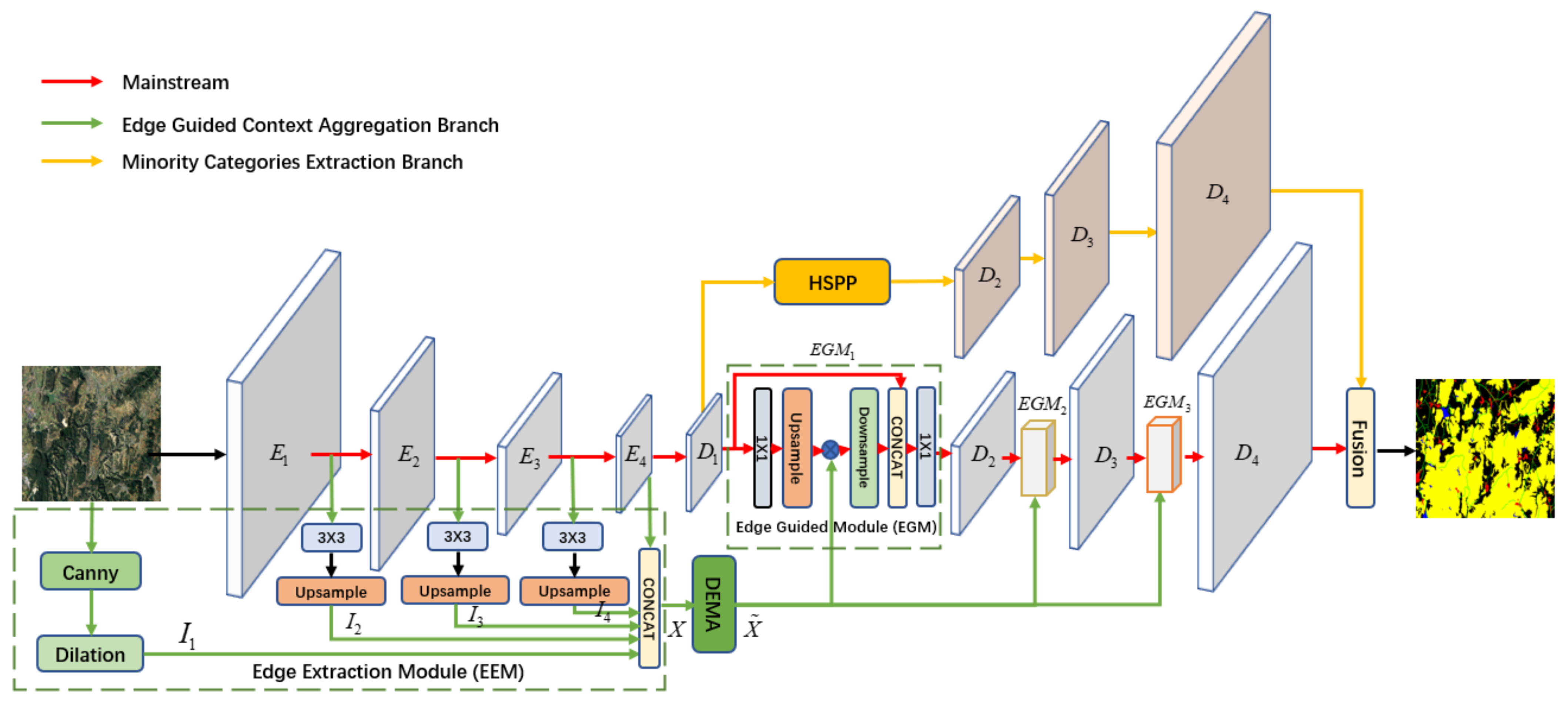
Article

Edge Guided Context Aggregation Network for Semantic Segmentation of Remote Sensing Imagery

1
The State Key Laboratory of Integrated Service Networks, Xidian University, Xi’an 710000, China
2
The State Key Laboratory of Geo-Information Engineering, Xi’an 710054, China
*
Author to whom correspondence should be addressed.
These authors contributed equally to this work.
Remote Sens. 2022, 14(6), 1353; https://doi.org/10.3390/rs14061353
Submission received: 25 January 2022 / Revised: 3 March 2022 / Accepted: 7 March 2022 / Published: 10 March 2022

Abstract

:
Semantic segmentation of remote sensing imagery (RSI) has obtained great success with the development of deep convolutional neural networks (DCNNs). However, most of the existing algorithms focus on designing end-to-end DCNNs, but neglecting to consider the difficulty of segmentation in imbalance categories, especially for minority categories in RSI, which limits the performance of RSI semantic segmentation. In this paper, a novel edge guided context aggregation network (EGCAN) is proposed for the semantic segmentation of RSI. The Unet is employed as backbone. Meanwhile, an edge guided context aggregation branch and minority categories extraction branch are designed for a comprehensive enhancement of semantic modeling. Specifically, the edge guided context aggregation branch is proposed to promote entire semantic comprehension of RSI and further emphasize the representation of edge information, which consists of three modules: edge extraction module (EEM), dual expectation maximization attention module (DEMA), and edge guided module (EGM). EEM is created primarily for accurate edge tracking. According to that, DEMA aggregates global contextual features with different scales and the edge features along spatial and channel dimensions. Subsequently, EGM cascades the aggregated features into the decoder process to capture long-range dependencies and further emphasize the error-prone pixels in the edge region to acquire better semantic labels. Besides this, the exploited minority categories extraction branch is presented to acquire rich multi-scale contextual information through an elaborate hybrid spatial pyramid pooling module (HSPP) to distinguish categories taking a small percentage and background. On the Tianzhi Cup dataset, the proposed algorithm EGCAN achieved an overall accuracy of 84.1% and an average cross-merge ratio of 68.1%, with an accuracy improvement of 0.4% and 1.3% respectively compared to the classical Deeplabv3+ model. Extensive experimental results on the dataset released in ISPRS Vaihingen and Potsdam benchmarks also demonstrate the effectiveness of the proposed EGCAN over other state-of-the-art approaches.

1. Introduction

Semantic segmentation is a typical computer vision problem that processes raw data such as RGB images, to be specific, converting them into masks with different highlighted regions of interest where each pixel of the image is assigned as a unique category label. In recent years, semantic segmentation has become one of the key issues in remote sensing imagery parsing for its widespread applications, including road extraction [1,2], urban planning [3,4], object detection [5,6], and change detection [7], to name a few.
Traditional segmentation methods mainly applied handcrafted features to assign pixel-wise category labels, ranging from classic approaches such as logistic regression [8], distance measures [9] and clustering [10], to more superior models based on machine learning such as the support vector machine (SVM) [11], random forest (RF) [12], conditional random fields (CRFs) [13], and multi layer perceptron (MLP) [14]. Nevertheless, due to the restricted dependency extraction and expressive ability of the above mentioned models based on handcrafted descriptors, these methods failed to achieve considerable performance in challenging cases.
For the past few years, DCNNs have been successful in natural image semantic segmentation and achieved excellent performance [15]. The CNN-based methods formulate the trainable tasks as an end-to-end paradigm and contain the powerful feature representation. One solution concentrates on designing an encoder–decoder architecture [16,17,18,19], which can keep more detailed information and obtain clearer object edges by gradually fusing low-level and high-level semantic features. Another solution is to exploit the elaborate contextual information. For instance, different-scale dilated convolutional layers or pooling functions are appended to the top of the network to incorporate multi-scale contexts and features in certain works [20,21,22]. There are several studies [23,24,25] to aggregate richer context information to invent large-size kernels or explore a context encoding module.
To enhance the discriminant ability of feature representations, the attention mechanism was introduced into semantic segmentation [26,27]. The attention mechanism models the internal process of biological observation, a mechanism that aligns internal experience and external sensation to increase the fineness of observation in some salient areas [28,29]. It is also well known that attention plays a vital role in human perception [30,31]. Attention not only tells where to focus, but also improves the representation of meaningful areas. With the help of the powerful semantic feature expression ability brought by the attention mechanism, the accuracy of semantic segmentation has been further improved [32,33].
Based on the success of CNNs in processing natural image semantic segmentation, they have been widely explored for semantic segmentation of RSI [34,35]. In general, compared with natural images, remote sensing images are featured by complex data attributes, and various types of ground objects are diverse and easy to mix. Due to diverse topological shapes and variable scales, the semantic segmentation of RSI encounters barricades to some extent. Although the existing DCNN models perform well, semantic labeling on RSI is still challenging and difficult. Several solutions like multi attention network [36], adaptive tree CNN [37], and multi-source data fusion [38] for semantic segmentation of RSI are proposed in several research works. However, most of the current algorithms focus on learning a complicated mapping through an end-to-end DCNN, neglecting to consider and analyze the segmentation of the categories taking a small percentage of pixels in RSI, limiting the performance of RSI semantic segmentation. For example, road elements in RSI usually account for a relatively low proportion and the scale of road distribution is variable, making it difficult to effectively extract road features through exploiting CNNs and resulting in low road segmentation accuracy. Meanwhile, most of the current algorithms show a similar problem in modeling contextual information. To solve this issue, many researches have been conducted to analyze contextual dependencies, and the existing solutions are generally classified into two types. One approach is to utilize a pyramid module that integrates multi-scales feature information just like atrous spatial pyramid pooling (ASPP) in Deeplab. Another approach is to express long-interdependence from a channel or spatial aspect, such as the Non Local module. However, these current methods lack specific prior along the edge areas to aggregate contextual information.
In this paper, a novel edge guided context aggregation network (EGCAN) is proposed for semantic segmentation of RSI to address the aforementioned issues. The Unet is adopted as backbone network to generate a dense prediction containing features of all object categories. Meanwhile, an edge guided context aggregation branch and minority categories extraction branch are presented in the proposed framework EGCAN according to their roles respectively. Specifically, the edge guided context aggregation branch contains three modules: edge extraction module (EEM), dual expectation maximization attention module (DEMA), and edge guided module (EGM). EEM estimates the binary edge information of remote sensing images, then the edge information and the global semantic features with different scales extracted from encoder part of the backbone are incorporated and fed into DEMA for sufficient context aggregation. Based on that, the edge area attention map generated by DEMA is fed back to EGM embedding in the different parts of decoder process to emphasize those error-prone pixels in the edge regions. Thus, the edge guided context aggregation branch can keep global semantic comprehension and enhances the representation of the edge features along the spatial and channel dimensions. Meanwhile, the minority categories extraction branch contains a hybrid spatial pyramid pooling module (HSPP), which is presented to acquire rich multi-scale contextual information to distinguish categories which take a small percentage and background; thus, a better segmentation result is achieved on the minority categories. Extensive experiments on the dataset released in the TianZhi Cup Artificial Intelligence Challenge, ISPRS Vaihingen, and Potsdam benchmarks demonstrate that the proposed algorithm can effectively improve the accuracy of semantic segmentation of RSI.
The main contributions of this paper are summarized as follows:
  • A novel architecture named edge guided context aggregation network (EGCAN) is proposed for RSI semantic segmentation. The advantage of the proposed network is that the edge information is employed as a priori knowledge to guide remote sensing image segmentation. The edge information is beneficial for effectively distinguishing background and different categories, especially the categories occupying a small percentage.
  • A novel edge guided context aggregation branch is invented containing three modules, edge extraction module (EEM), dual expectation maximization attention module (DEMA) and edge guided module (EGM) to promote the accuracy of edge predictions, which enhances edge feature interdependencies and representation ability of the network along the spatial and channel directions.
  • A hybrid spatial pyramid pooling (HSPP) module is investigated in minority categories segmentation branch, which is comprised of different-scale dilated convolutions and pooling operations to capture rich multi-scale contextual information for improving the proposed model’s discriminative capability of minority categories.
  • Extensive experimental results on the dataset released in the TianZhi Cup Artificial Intelligence Challenge, ISPRS Vaihingen, and Potsdam benchmarks demonstrate the superiority of the proposed EGCAN over other state-of-the-art approaches.

2. Related Work

Semantic segmentation is a fundamental and challenging task in the field of computer vision involving a deep semantic understanding of various types of images. In this section, methods regarding semantic segmentation of nature scenes and remote sensing images and attention mechanism relevant to our proposed method are reviewed.

2.1. Semantic Segmentation

As an extension of classic CNN, the fully convolutional neural network (FCN) that can learn the mapping relationship between pixels without extracting region suggestions aims to make classic CNN accept images of any size as input. Long et al. [15] built the first FCN in semantic segmentation. Utilizing the powerful representation learning ability of CNNs, FCN greatly surpassed the traditional methods based on hand-crafted features. Subsequently, several model variants were proposed to boost contextual extraction. For example, PSPNet [21] designed a pyramid pooling module (PPM) to exploit the global context information and produced a superior pixel-level prediction result. DeeplabV2 [20] aggregated contextual information via an astrous spatial pyramid pooling (ASPP) module constituted of parallel dilated convolutions with different dilated rates. Deeplabv3 [22] extended ASPP with image-level feature to further obtain more contexts. Meanwhile, to reduce computational complexity, FastFCN [39] further introduced the joint pyramid up sampling (JPU) module as a substitute for extended convolution.
Typically, the encoder–decoder networks, such as convolutional networks for biomedical image segmentation (Unet) [17], encoder–decoder with atrous separable convolution for semantic image segmentation (DeepLabv3+) [40], a deep convolutional encoder–decoder architecture for image segmentation (SegNet) [18], and semantic prediction guidance for scene parsing (SPGNet) [41], established skip-connection, explicitly connecting encoder layers with decoder layers to gradually recover the spatial information, thus improving the models’ accuracies and addressed the problem of vanishing gradients. Similarly, Yu et al. [42] preserved rich spatial information and obtained a larger receiving field by proposing spatial and context paths, which solved the high computational cost associated with high-resolution feature maps in the U-shaped architecture.

2.2. Attention Mechanism

The attention mechanism intended to elevate the effectiveness of certain models is widely applied to machine translation, image classification, semantic segmentation, etc. The attention-based networks and their variants have been proposed to tackle the challenge in semantic segmentation [43,44]. Inspired by the outstanding performance of the attention mechanism in machine translation originally proposed by Bahdanau et al. [43], a Squeeze-and-Excitation Network (SENet) was proposed by Hu et al. [44], introducing global average pooling to aggregate the feature maps. Then, the feature maps were simplified into a single channel descriptor, thus highlighting the most distinguishing features. Inspired by the self-attention mechanism, to explore the long-range dependency encouraged by attention-based networks utilizing Non Local module in semantic segmentation, the Double Attention Networks (AA2-Net) [45], Dual Attention Network (DANet) [27], Point-wise Spatial Attention Network (PSANet), Object Context Network (OCNet) [46], and Co-occurrent Feature Network (CFNet) [47] were proposed. Later on, Li et al. [48] further enhanced the attention mechanism’s efficiency by combining self-attention and EM algorithm [49].

2.3. RSI Semantic Segmentation

The development of remote sensing technology has made it easy to obtain a large number of high-quality remote sensing images. Meanwhile, encouraged by the progress made by deep learning (DL) applied in natural image processing, there indicates a promising prospect for a variety of DL based methods to be applied in RSI, thus improving understanding of the context. To address the different orientations of the RSI, Marcos et al. [50] developed a Rotation Equivariant Vector Field Network (RotEqNet) encoding rotation equivariance. Furthermore, Liu et al. [51] proposed that multiscale contexts captured by CNN encoder could be aggregated to improve the labeling coherence and low-level features from CNN’s shallow layers for helping refine the objects. Both adaptive hierarchies and a deep neural network are used in a unified deep learning structure in the structure of TreeUNet. Likewise, a similar unified deep learning structure that combines decision trees and CNNs has been proposed in the work of ANT [52]. Liu et al. [51] proposed a novel end-to-end self-cascaded network (ScasNet) that promoted the labeling coherence with sequential global-to-local contexts aggregation, especially for confusing artificial objects. Superpixel-enhanced Deep Neural Forest (SDNF) [53] was proposed to tackle difficulties in distinguishing ground object categories due to the complexity of ground objects’ spectrum. Furthermore, semantic segmentation and semantically informed edge detection were combined to clarify class boundaries in the work of Marmanis et al. [54].

3. The Proposed Method

3.1. Overview

As shown in Figure 1, the proposed edge guided context aggregation network (EGCAN) consists primarily of three parts according to the effects of each part: the mainstream Unet, which combines encoder parts E 1 , E 2 , E 3 , E 4 and decode parts D 1 , D 2 , D 3 , D 4 ; the edge guided context aggregation branch, which contains edge extraction module (EEM), dual expectation maximization attention module (DEMA), and edge guided module (EGM); and the minority categories extraction branch. In view of the edge guided context aggregation branch, firstly, the EEM is employed to obtain the edge feature map. Then, the edge information I 1 derived from the segmentation result of canny with morphological dilation operation and the various semantic information I 2 , I 3 , I 4 with different scales which were generated from four stages of the backbone Resnet101 [55], are combined together. After that, the proposed DEMA is utilized to aggregate the context of edge feature map. The result of DEMA is fed into the decoder parts noted as EGM, to verify the region of the object edges and relearn them in a gradual manner. For the minority categories extraction branch, the hybrid spatial pyramid pooling (HSPP) is exploited to obtain multi-scale spatial information through adjusting scale and rate parameters. Following that, the same decoder part of the mainstream except the edge guided module is shared to get the minority categories feature map. Lastly, the features of the mainstream and the minority categories extraction branch were fused by an ensemble way to obtain a better segmentation result.

3.2. Edge Guided Context Aggregation Branch

3.2.1. Edge Extraction Module (EEM)

Since the edge feature information are utilized to drive the procedure of edge context aggregation and they connect with the mainstream semantic features, EEM adopts the middle representations information from the backbone as its input directly. This step is beneficial to fully utilize low level feature and high level semantic information when the connections between the mainstream and the edge stream are created to allow different levels of information to flow over the network. As shown in Figure 1, the feature maps were obtained from every stage of the backbone Resnet101 by a 3 × 3 convolution. The following upsampling operation directly utilized bilinear interpolation to acquire the same size feature as the input feature maps. After that, the edge extraction module obtained the feature maps I 2 , I 3 , I 4 . In order to get more, clearer edge information and feed the edge information into the decoder part of the network, canny and dilation operations were utilized to get the binary edge map I 1 . As shown in Figure 1, the EEM offers a concatenate operation to get the binary edge map and the feature maps from backbone together.
X = ψ ( I 1 , I 2 , I 3 , I 4 )
where X denotes the result of the EEM. ψ denotes a series of operations: concatenate, 1 × 1 convolution, BatchNorm and Sigmoid.

3.2.2. Dual Expectation Maximization Attention Module (DEMA)

The ddge guided context aggregation branch introduces the expectation maximization algorithm into the self-attention mechanism, which runs the attention mechanism through a set of compact base set instead of every pixel position of the whole image. The expectation maximization algorithm refers to finding the maximum likelihood estimation or the maximum posterior estimation of parameters in a probabilistic model, which depends on hidden variables that cannot be observed directly. The main steps of the algorithm are step E and step M [48]. As illustrated in Figure 2, step E is purposed to calculate the spatial attention map Z, using the existing estimate of the hidden variable to calculate its maximum likelihood estimate. Step M is purposed to maximize the maximum likelihood value μ obtained in step E to calculate the value of the parameter. The parameter estimates gained at step M are used in the following step E to calculate the expectation. The algorithm executes step E and step M alternately until the convergence criterion is satisfied.
As illustrated in Figure 2, a dual expectation maximization attention (DEMA) module was developed to explore the feature correlations along both spatial and channel dimensions. The feature map X, which is the output of edge extraction module, has been considered with a size of C × H × W , where C represents the number of channels, and H and W denote the height and width, respectively.
First, the SEMA module reshapes X into a simplified form of N × C , where N = H × W . After that, the bases μ is initialized as K vectors of length C, then the EM iteration step is executed (step E generates the attention map, step M updates μ ). In the t-th iteration, the spatial attention map Z is expressed in the form of exponential inner product as:
Z n k ( t ) = softmax λ X n μ k ( t 1 ) T
where 1 n N and 1 k K and λ is a hyper-parameter to control Z. Next, μ can be updated through Z to:
μ k ( t ) = Z n k ( t ) X n m = 1 N Z m k ( t )
In order to ensure that the learning of μ is stable, L2 norm is adopted to normalize μ in each update. After T iterations, the feature X ˜ s about spatial dimension can be obtained by reconstructing the final Z and μ as:
X ˜ s = Z ( T ) μ ( T )
Similar to SEMA, the CEMA module reshapes X ˜ s to R C × N . Then, base ν is initialized to R N × J . Next, the EM iteration step is performed. In the t-th iteration, the channel attention map F is represented in the form of exponential inner product as:
F c j ( t ) = softmax θ X ˜ c v j ( t 1 ) T
where 1 c C and 1 j J and θ is a hyper-parameter to control F. Next, ν can be renewed according to F to:
ν j ( t ) = F c j ( t ) X c m = 1 C F m j ( t )
To make sure that the learn of ν is stable, L2 norm is also adopted to normalize ν in each iteration. After T iterations, the feature X ˜ c can be obtained by reconstructing the final F and ν as:
X ˜ c = F ( T ) ν ( T )
Ultimately, refined features X ˜ s and X ˜ c are reshaped to R C × H × W and combined with X to generate the edge area attention map.

3.2.3. Edge Guided Module (EGM)

As previously stated, the edge of remote sensing imageries contains pixels that are hard to distinguished in the semantic segmentation task. Thus, the results of DEMA were sent into the EGM, the decoder part of the mainstream. The EGM retrains the pixels along the region of the edge and remodels the edge feature space. This strategy helps to improve the abilities of discriminatory for edge pixels. As shown in Figure 1, the result of the encoder part of EGCAN noted as D n is fed it into EGM. The edge guided module gets τ D n where τ denotes 1 × 1 convolution, BatchNorm, and ReLu. Following that, an upsample procedure is performed. In order to maintain the same dimensions the upsampling ratio n n ( n is predetermined was set to 16, 8, 2 in E G M 1 , E G M 2 , E G M 3 , respectively). The edge feature is then used to reconstruct as
f D n = τ D n X ˜
where ⊗ denotes elementwise production, and X ˜ is the result of DEMA. Guided by edge area attention map, f D n accentuates the pixels along the edge which is hard to distinguish. Next, the edge guided module combines f D n with D n by the means of downsample procedure and concatenate operation. Meanwhile, the downsample ratio m m is set to be the same as the upsample operation. In order to effectively utilize the advantages of the edge area attention map, the decoder part of EGCAN gradually enhances the representation ability of features
f n = ξ Cat f D n , D n
where ξ formed by convolution layers (i.e., 1 × 1 convolution, BatchNorm, and ReLU), which are used to reduce the number of channels and maintain resolution, respectively. “Cat” refers to a concat operation used to fuse f D n and D n . f n is the output of E G M n .

3.3. Minority Categories Extraction Branch

As stated in the introduction, the current algorithms neglect to consider and analyze the segmentation for categories which take a small percentage of remote sensing imageies, which makes it difficult for existing CNN-based methods to effectively extract contextual features. At the same time, due to the diverse topology shapes and different distribution scales for minority categories elements, the segmentation accuracy of minority categories is further limited. Global average pooling and dilated convolution operation have been proven to be powerful tools for capturing contextual characteristics. Besides this, it is beneficial to obtain multi-scale spatial information by adjusting scale and rate parameters. Accordingly, a hybrid spatial pyramid pooling (HSPP) module is investigated in minority categories extraction branch of the proposed EGCAN network.
Figure 3 depicts an illustration of the HSPP module, which is comprised of two parallel different-scale dilated convolutions and global average pooling operations. The input of this module is from the output feature of the dilated Resnet101 backbone network. To reduce the computational complexity, the HSPP employs 1 × 1 convolution to reduce the channel dimension of the corresponding feature for each pooling operation, while dilated convolutions apply a smaller number of filters. The following upsampling directly utilize bilinear interpolation to acquire the same size feature as the input feature map. Then, different scales and rates of features are concatenated as the final hybrid spatial pyramid feature. At the end of the proposed network, EGCAN fuses the results of the mainstream and the minority categories extraction branch via an ensemble strategy by voting.

4. Experiments and Results

In this section, the effectiveness of the proposed method is validated through a variety of datasets. Section 4.1 introduces fundamental experiment conditions and settings. A brief description of datasets utilized for the benchmark is shown in Section 4.2. Introduction for evaluation metrics can be found in Section 4.3. In Section 4.4, the effectiveness of the model EGCAN was evaluated in the Tianzhi Cup AI Challenge Dataset, ISPRS Vaihingen, and Potsdam dataset. Experimental results comprising the comparison of the proposed method and other classic methods can also be found in Section 4.4.

4.1. Experimental Settings

The hardware and system configuration for the laboratory server intended for our experiments is shown in Table 1. Essential packages for the experiment include Python 3.6, CUDA 9.0, Pytorch 1.1.0, and others.
Certain operations for images like rotation, flip, brightness adjustment, and noise addition were adopted randomly in data augmentation to improve the generalization performance of the proposed method. Furthermore, due to sample imbalance in certain datasets, sample equalization was introduced to enhance the effectiveness of the training process.
In order to avoid problems caused by hardware resource limitations, the images were cropped into patches of 512 × 512 resolution with a stride of 256 pixels for both rows and columns. For the Tianzhi Cup AI Challenge Dataset, 6422 images are used for training. For the ISPRS Vaihingen and Potsdam Challenge Datasets, the training set contains 864 and 9580 images, respectively. Adam optimization was adopted with the batch size 8 in the training process. The learning rate is initialized at 0.00002 with the polynomial function of power = 1.5 as the decay policy. The total training epoch is set as 100. Based on the experimental settings description above, the training time for the proposed method is approximately 24.3 mins using the Tianzhi Cup AI Challenge Dataset, 3.5 mins using the ISPRS Vaihingen Challenge Dataset, and 38.8 mins using the ISPRS Potsdam Challenge Dataset, respectively.

4.2. Dataset Description

The proposed method was validated on the dataset released in the TianZhi Cup Artificial Intelligence Challenge, ISPRS Vaihingen, and Potsdam benchmarks.The ground truth of the TianZhi dataset comprises five different common land cover categories: farmland, roads, water, vegetation, and backgrounds that denotes all other categories that differ from the above four categories. ISPRS datasets include the six most common land cover classes, impervious surfaces (imp_surf), buildings (building), low vegetation (low_veg), trees (tree), cars (car), and clutter/background (clutter).
The Tianzhi Cup AI Challenge Dataset consists of a pair of 23 RSIs of 7400 × 4950 resolution and corresponding ground truth semantic labels. Each image contains three channels of red (R), green (G), and blue (B). Following the contest instructions, 12 of them are used for training, 6 of them are used as validation data, and the remaining RSI are used for testing.
The ISPRS Vaihingen Challenge Dataset contains a variety of independent buildings and small multi-storey buildings, involving 33 orthorectified patches of different sizes acquired by a near-infrared–green (G)–red (R) aerial camera over the town of Vaihingen (Germany). Each image is accompanied by a corresponding DSM representing the absolute heights of pixels. The average size of the tiles is 2494 × 2064 pixels with a spatial resolution of 9 cm. DSM is not used in these experiments. Recently, the challenge organizer opened the ground truths of all the images. Among the previously opened ground truths, 12 annotated images were used to train the networks, 4 images (ID 5, 7, 23, and 30) were used to validate performance, and the remaining 17 images were used as a test set to evaluate the segmentation generalization accuracy.
The ISPRS Potsdam Challenge Dataset contains 38 orthorectified same-size patches of size 6000 × 6000 pixels with a spatial resolution of 5 cm over the town of Potsdam (Germany). This dataset offers near-infrared, red, green, and blue channels together with the DSM and normalized DSM (NDSM). There are 20 images in the training set, 4 images (ID 2_11, 4_10, 5_11, and 7_8) in the validation set, and 14 images in the test set.

4.3. Evaluation Metrics

The performance of the proposed method was evaluated by overall accuracy (OA), mean Intersection over union (mIoU), and F 1 score.
The overall accuracy as an intuitive metric computes a ratio of the amount of correctly classified pixels and the total number of pixels, standing for a general assessment result for overall pixels. The OA can be calculated as follows:
O A = i = 0 k p i i i = 0 k j = 0 k p i j
The intersection over union (IoU) represents a ratio of the intersection of pixels predicted to be of a specific category and the ground truth pixels of that category and their union. The mIoU can be derived by averaging the IoU for all the label categories besides background. It is assumed that there are total k + 1 categories (from 0 to k, and 0 represents the Backgrounds), while p i j stands for the number of pixels belonging to category i and being predicted as category j. The mIoU can be calculated as follows:
m I o U = 1 k + 1 i = 1 k p i i i = 1 k p i j + j = 1 k p j i p i i
F 1 score is defined as the harmonic mean of recall and precision, and can be calculated as follows:
F 1 = 2 r e c a l l × p r e c i s i o n r e c a l l + p r e c i s i o n
Recall and precision, representing completeness and correctness, respectively, for class i are calculated as follows:
r e c a l l = T P T P + F N , p r e c i s i o n = T P T P + F P
True Positive (TP), False Positive (FP), True Negative (TN), and False Negative (FN) are the four most basic metrics, in which Positive and Negative represent the prediction whether pixels belong to one class, while True and False represent the authenticity of this prediction, For example, TP represents the number of pixels predicted to be one class and belongs to this class. Assume that there are total k + 1 classes (from 0 to k), and p i j stands for the number of pixels belonging to class i but being predicted as class j, for class i, they can be derived as:
T P = P i j , F P = j i P j i , T N = j i P j j , F N = j i P i j

4.4. Experimental Results

Quantitative comparisons between other approaches and the proposed method on the Tianzhi testing dataset are conducted by metrics of OA and mIoU. In the TianZhi Cup dataset, the proportion of road elements is the lowest, so the minority categories extraction branch of the proposed network is mainly used to distinguish road elements. As shown in Table 2, the proposed method ranks first in OA and mIoU among six other classic methods and achieves 84.1% in OA and 68.1% in mIoU on the Tianzhi testing dataset. Meanwhile, the proposed method performs the best in categories of farmland and roads by a relatively large margin compared to other networks, which denotes the proposed method’s effectiveness, especially for the minority category. From Figure 4, it can be seen that our method achieves the best visualization effect, reflecting the consistency of the numerical results. In view of road element, the proposed method provides a more complete and accurate segmentation along the edge of the road. Meanwhile, misclassified pixels along the edge of objects take a smaller proportion.
To further test the effectiveness of the proposed EGCAN, comparisons with competitors’ methods on the two challenging Vaihingen and Potsdam benchmarks were carried out. In the Vaihingen and Potsdam benchmarks, the proportion of car elements is the lowest, so the minority categories extraction branch of the proposed network in Vaihingen and Potsdam benchmarks is mainly used to distinguish car elements. The competitors’ methods on the two challenging Vaihingen and Potsdam benchmarks contain: SVL_1, SVL_3, DST_2, DST_5, UZ_1, RIT_L7, ONE_7, ADL_3, DLR_10, CASIA_2, BKHN_10, TreeUNet, SWJ_2. Cascade denotes the Cascade-Edge-FCN and Correct denotes the Correct-Edge-FCN [56]. EDENet denotes the edge distribution-enhanced semantic segmentation neural network [57]. Table 3 and Table 4 show the quantitative comparisons on the Vaihingen and Potsdam testing dataset. Correspondingly, visual comparisons are shown in Figure 5 and Figure 6. In Table 3, the proposed EGCAN obtains an OA of 91.0% and Mean F1 of 89.7%. The Mean F1 of ours is listed in third place. From this, it can be seen that our method provides a very competitive result. As for the Potsdam testing dataset, the proposed method can acquire 93.0% in MeanF1, exceeding all the comparisons listed in Table 4. Moreover, the OA is second only to SWJ2. From Figure 5 and Figure 6, our method still has significant advantages in dealing with complex feature images.

5. Disussion

5.1. Ablation of Edge Extraction Module

As shown in Table 5, four experiments were designed to evaluate the performance of edge extraction module. In experiment (a), the Unet is adopted as baseline for semantic segmentation of remote sensing imageries. In experiment (b), the sEEM is introduced into the baseline where the sEEM denotes single-scale edge extraction module which only utilizes one intermediate feature from the decode part of the backbone, Resnet101. It means that information I 4 instead of I 2 or I 3 is used in the following ablation experiments. In experiment (c), all information I 2 , I 3 , I 4 from each stage of Resnet101 are used to aggregate context from multi-scale features. Based on experiment (c), canny and dilation operations are utilized to get clearer edge features. Then, the clearer edge features are fed into the decoder part of EGCAN. In view of the results, the improvement using sEEM alone is not significant, only a 2.1% increase on mIoU. However, the proposed method achieves 4.2% improvement by EEM (without canny and dilation), thus proving the effectiveness of the multi-scale context extraction. Furthermore, a better result of 63.2% on mIoU is obtained by adding canny and dilation operations in experiment (d), which clearly validates the significance of canny and dilation operations. From experiment (a) to experiment (d), the proposed network gets more and more edge information when the baseline Unet gradually adds other modules which enhance the representations ability of the network along the edge of different categories.
Visual comparisons are shown in Figure 7. The first column is the input and the second column is the the label of input. The third to sixth columns show the results from experiments a, b, c, and d. According to the visual results, EEM effectively extracts rich feature information especially with the help of canny and dilation operations. From the first row and second row, it shows the improvement of the edge extraction, especially on the road element. However, from the second row to third row, it can be seen that the proposed method still performs well when the context of remote sensing images become more and more complicated.

5.2. Ablation of Dual Expectation Maximization Attention Module

To evaluate the effect of each component of the proposed approach, an ablation study is conducted on the Tianzhi dataset. As shown in Table 6, the baseline network only utilizing the dilated Resnet101 as backbone framework can achieve 59.4% in mIoU score. Then, the individual SEMA module or CEMA module are added to the backbone network to explore the multi-category segmentation. It can be seen that the SEMA or CEMA module alone would yield 60.6% or 61.1%, which can bring 2.0% or 2.8% improvement, respectively, thus proving the effectiveness of a single SEMA or CEMA module. Subsequently, three different ways were compared to arrange these two attention modules. As shown in Table 6, ‘SEMA || CEMA’ denotes that SEMA and CEMA module are set in the paralleled structure. ‘CEMA → SEMA’ stands for the structure where a SEMA module follows a CEMA module. ‘SEMA → CEMA’ denotes the structure where a CEMA module follows a SEMA module. Compared with the baseline result, involving SEMA and CEMA modules simultaneously and placing them in a cascade structure will bring 5.7% improvement. Then, consider placing SEMA and CEMA module in a paralleled structure. In the case where the SEMA module follows the CEMA module, 8.9% improvement can be achieved. In the case where the CEMA module follows the SEMA module, the improvement will be 9.9% and yield 65.3% in mIoU. In order to get a better result, the DEMA module of the EGCAN network applies this arrangement, which enhances edge feature interdependencies and representations ability of the network along the spatial and channel directions. Quantitative visualization results are shown in Figure 8. Obviously, DEMA enhances our model’s sensitivity to edges of various scales and enables the pixels of the same class to achieve similar gains.

5.3. Influence of Edge Guided Module

As shown in Table 7, the proposed EGM enhances the model’s mIoU by 0.4%, 1.3%, and 2.5%, respectively, confirming their efficiency in retraining the pixels along the region of the edge and remodeling the edge feature space. The promotion brought by EGM3 is more distinct than others, considering that the feature map in this module processes the largest resolution to maintain edge information. Quantitative visualization results are shown in Figure 9. From the third column to the sixth column, the results of semantic segmentation get better and better because of progressively relearning error-prone pixels by EGMs to enhance our model’s ability to distinguish different classes.

5.4. Effections of Hybrid Spatial Pyramid Pooling Module

Based on the statistics of the total number of categories, the proportion of road category is usually smaller, owing to the inherent narrow and long distribution paradigm. Meanwhile, the scale of road distribution is variable, making it difficult to adequately extract road characteristics and making the segmentation accuracy low. The proposed EGCAN method considers to employ another branch designing the HSPP block to fulfill the road segmentation. The results are shown in Table 8. In particular, ASPP uses parallel convolution operation to extract multi-scale semantic features; its ability for driving mainstream context aggregation is not completely realized. Our model outperforms ASPP by 1.39% in terms of accuracy. In comparison to prior self-attention-based strategies, such as Non Local, RCCA, and DNL, HSPP successfully helps to reduce the negative effect of intra-class inconsistency, resulting in significant mIoU improvements of 4.6%, 5.0%, and 1.4%, respectively. The experimental result shows that considering both the mainstream segmentation and the road extraction segmentation can further produce better prediction. The mIoU score reaches 68.1%, which is 1.4% higher than the second best result. Quantitative visualization results are shown in Figure 10.

6. Conclusions

By considering abundant edge information and low-percentage categories of segmentation, a novel edge guided context aggregation network (EGCAN) designed for semantic segmentation of RSI breaks the barricades of the performance of RSI semantic segmentation, proving that the structure of the proposed method works and performs well. Essentially, an edge guided context aggregation branch was developed to promote the accuracy of edge predictions. Then, a hybrid spatial pyramid pooling (HSPP) module was investigated in the minority categories segmentation branch, which is utilized to capture rich multi-scale contextual information for improving EGCAN’s discriminative capability of minority categories. As a result, our proposed method performed the best on the Tianzhi Cup AI Challenge Dataset and is among the best on the ISPRS Vaihingen and Potsdam Challenge Datasets.
Nevertheless, there are still several challenging issues to be addressed. First of all, the annotations of the dataset need to be more precise to improve the semantic segmentation performance. Moreover, computing power is consumed more when the model becomes larger and larger. Thus, how to balance the performance of semantic segmentation and the computer power is an important direction of future research. Furthermore, whether some smaller edge extraction module can replace the edge guided context aggregation branch to obtain better results in semantic segmentation is a direction worth studying as well.

Author Contributions

J.L. and Z.L. (Zhiqiang Liu) conceived and designed the study; Z.L. (Zhiqiang Liu) performed the experiments; R.S. shared part of the experiment data; W.L. and Y.L. analyzed the data; Z.L. (Zhiqiang Liu) and J.L. wrote the paper. R.S. and C.W. reviewed and edited the manuscript. Z.L. (Zan Li) and J.L. provided the funding. All authors have read and agreed to the published version of the manuscript.

Funding

This research was funded in part by the National Nature Science Foundation of China (no. 61901343), the state Key Laboratory of Geo-Information Engineering, (no. SKLGIE2020-M-3-1), the China Postdoctoral Science Foundation (no. 2017M623124), and the China Postdoctoral Science Special Foundation (no. 2018T111019). The project was also partially funded by the science and technology on space intelligent control laboratory ZDSYS-2019-03 and the Fundamental Research Funds for the Central Universities JB190107. It was also partially funded by the National Nature Science Foundation of China (no. 61571345, 61671383, 91538101, 61501346 and 61502367), the 111 project (B08038), and the Innovation Fund of Xidian University (no. 10221150004), and the Government-Business-University-Research Cooperation fundation between Wuhu and Xidian XWYCXY-012021002-HT.

Institutional Review Board Statement

Not applicable.

Informed Consent Statement

Not applicable.

Data Availability Statement

Publicly available datasets were analyzed in this study. The data can befound here: [http://www2.isprs.org/commissions/comm3/wg4/2d-semlabel-vaihingen.html] (accessed on 10 December 2017) and [http://www2.isprs.org/commissions/comm3/wg4/2d-semlabel-potsdam.html] (accessed on 10 December 2017).

Conflicts of Interest

The authors declare no conflict of interest.

References

  1. Maboudi, M.; Amini, J.; Malihi, S.; Hahn, M. Integrating fuzzy object based image analysis and ant colony optimization for road extraction from remotely sensed images. ISPRS J. Photogramm. Remote Sens. 2018, 138, 151–163. [Google Scholar] [CrossRef]
  2. Zhu, Z.; Li, X.; Xu, J.; Yuan, J.; Tao, J. Unstructured Road Segmentation Based on Road Boundary Enhancement Point-Cylinder Network Using LiDAR Sensor. Remote Sens. 2021, 13, 495. [Google Scholar] [CrossRef]
  3. Zhang, Q.; Seto, K.C. Mapping urbanization dynamics at regional and global scales using multi-temporal DMSP/OLS nighttime light data. Remote Sens. Environ. 2011, 115, 2320–2329. [Google Scholar] [CrossRef]
  4. Abdollahi, A.; Pradhan, B.; Shukla, N.; Chakraborty, S.; Alamri, A. Multi-Object Segmentation in Complex Urban Scenes from High-Resolution Remote Sensing Data. Remote Sens. 2021, 13, 3710. [Google Scholar] [CrossRef]
  5. Zhong, Y.; Han, X.; Zhang, L. Multi-class geospatial object detection based on a position-sensitive balancing framework for high spatial resolution remote sensing imagery. ISPRS J. Photogramm. Remote Sens. 2018, 138, 281–294. [Google Scholar] [CrossRef]
  6. Bai, L.; Li, Y.; Cen, M.; Hu, F. 3D Instance Segmentation and Object Detection Framework Based on the Fusion of Lidar Remote Sensing and Optical Image Sensing. Remote Sens. 2021, 13, 3228. [Google Scholar] [CrossRef]
  7. Ghosh, A.; Mishra, N.S.; Ghosh, S. Fuzzy clustering algorithms for unsupervised change detection in remote sensing images. Inf. Sci. 2011, 181, 699–715. [Google Scholar] [CrossRef]
  8. Rutherford, G.; Guisan, A.; Zimmermann, N. Evaluating sampling strategies and logistic regression methods for modelling complex land cover changes. J. Appl. Ecol. 2007, 44, 414–424. [Google Scholar] [CrossRef]
  9. Du, Q.; Chang, C.I. A linear constrained distance-based discriminant analysis for hyperspectral image classification. Pattern Recognit. 2001, 34, 361–373. [Google Scholar] [CrossRef]
  10. Maulik, U.; Saha, I. Automatic fuzzy clustering using modified differential evolution for image classification. IEEE Trans. Geosci. Remote Sens. 2010, 48, 3503–3510. [Google Scholar] [CrossRef]
  11. Gualtieri, J.A.; Cromp, R.F. Support vector machines for hyperspectral remote sensing classification. In 27th AIPR Workshop: Advances in Computer-Assisted Recognition; International Society for Optics and Photonics: Bellingham, WA, USA, 1999; Volume 3584, pp. 221–232. [Google Scholar]
  12. Pal, M. Random forest classifier for remote sensing classification. Int. J. Remote Sens. 2005, 26, 217–222. [Google Scholar] [CrossRef]
  13. Zhong, P.; Wang, R. A multiple conditional random fields ensemble model for urban area detection in remote sensing optical images. IEEE Trans. Geosci. Remote Sens. 2007, 45, 3978–3988. [Google Scholar] [CrossRef]
  14. Zhang, C.; Pan, X.; Li, H.; Gardiner, A.; Sargent, I.; Hare, J.; Atkinson, P.M. A hybrid MLP-CNN classifier for very fine resolution remotely sensed image classification. ISPRS J. Photogramm. Remote Sens. 2018, 140, 133–144. [Google Scholar] [CrossRef] [Green Version]
  15. Long, J.; Shelhamer, E.; Darrell, T. Fully convolutional networks for semantic segmentation. In Proceedings of the IEEE Conference on Computer Vision and Pattern Recognition, Boston, MA, USA, 7–12 June 2015; pp. 3431–3440. [Google Scholar]
  16. Wei, H.; Xu, X.; Ou, N.; Zhang, X.; Dai, Y. DEANet: Dual Encoder with Attention Network for Semantic Segmentation of Remote Sensing Imagery. Remote Sens. 2021, 13, 3900. [Google Scholar] [CrossRef]
  17. Ronneberger, O.; Fischer, P.; Brox, T. U-net: Convolutional networks for biomedical image segmentation. In International Conference on Medical Image Computing and Computer-Assisted Intervention; Munich, Germany, 5–9 October 2015, Springer: Cham, Switzerland, 2015; pp. 234–241. [Google Scholar]
  18. Badrinarayanan, V.; Kendall, A.; Cipolla, R. Segnet: A deep convolutional encoder-decoder architecture for image segmentation. IEEE Trans. Pattern Anal. Mach. Intell. 2017, 39, 2481–2495. [Google Scholar] [CrossRef]
  19. Romera, E.; Alvarez, J.M.; Bergasa, L.M.; Arroyo, R. Erfnet: Efficient residual factorized convnet for real-time semantic segmentation. IEEE Trans. Intell. Transp. Syst. 2017, 19, 263–272. [Google Scholar] [CrossRef]
  20. Chen, L.C.; Papandreou, G.; Kokkinos, I.; Murphy, K.; Yuille, A.L. Deeplab: Semantic image segmentation with deep convolutional nets, atrous convolution, and fully connected crfs. IEEE Trans. Pattern Anal. Mach. Intell. 2017, 40, 834–848. [Google Scholar] [CrossRef] [Green Version]
  21. Zhao, H.; Shi, J.; Qi, X.; Wang, X.; Jia, J. Pyramid scene parsing network. In Proceedings of the IEEE Conference on Computer Vision and Pattern Recognition, Honolulu, HI, USA, 21–26 July 2017; pp. 2881–2890. [Google Scholar]
  22. Chen, L.C.; Papandreou, G.; Schroff, F.; Adam, H. Rethinking atrous convolution for semantic image segmentation. arXiv 2017, arXiv:1706.05587. [Google Scholar]
  23. Peng, C.; Zhang, X.; Yu, G.; Luo, G.; Sun, J. Large kernel matters–improve semantic segmentation by global convolutional network. In Proceedings of the IEEE Conference on Computer Vision and Pattern Recognition, Honolulu, HI, USA, 21–26 July 2017; pp. 4353–4361. [Google Scholar]
  24. Zhang, H.; Dana, K.; Shi, J.; Zhang, Z.; Wang, X.; Tyagi, A.; Agrawal, A. Context encoding for semantic segmentation. In Proceedings of the IEEE Conference on Computer Vision and Pattern Recognition, Salt Lake City, UT, USA, 18–23 June 2018; pp. 7151–7160. [Google Scholar]
  25. Panboonyuen, T.; Jitkajornwanich, K.; Lawawirojwong, S.; Srestasathiern, P.; Vateekul, P. Transformer-Based Decoder Designs for Semantic Segmentation on Remotely Sensed Images. Remote Sens. 2021, 13, 5100. [Google Scholar] [CrossRef]
  26. Zhao, H.; Zhang, Y.; Liu, S.; Shi, J.; Loy, C.C.; Lin, D.; Jia, J. Psanet: Point-wise spatial attention network for scene parsing. In Proceedings of the European Conference on Computer Vision (ECCV), Munich, Germany, 8–14 September 2018; pp. 267–283. [Google Scholar]
  27. Fu, J.; Liu, J.; Tian, H.; Li, Y.; Bao, Y.; Fang, Z.; Lu, H. Dual attention network for scene segmentation. In Proceedings of the IEEE/CVF Conference on Computer Vision and Pattern Recognition, Long Beach, CA, USA, 15–20 June 2019; pp. 3146–3154. [Google Scholar]
  28. Vaswani, A.; Shazeer, N.; Parmar, N.; Uszkoreit, J.; Jones, L.; Gomez, A.N.; Kaiser, L.; Polosukhin, I. Attention is all you need. arXiv 2017, arXiv:1706.03762. [Google Scholar]
  29. Pham, T. Semantic Road Segmentation using Deep Learning. In Proceedings of the 2020 Applying New Technology in Green Buildings (ATiGB), Da Nang, Vietnam, 12–13 March 2021; pp. 45–48. [Google Scholar]
  30. Rensink, R.A. The dynamic representation of scenes. Vis. Cogn. 2000, 7, 17–42. [Google Scholar] [CrossRef]
  31. Corbetta, M.; Shulman, G.L. Control of goal-directed and stimulus-driven attention in the brain. Nat. Rev. Neurosci. 2002, 3, 201–215. [Google Scholar] [CrossRef]
  32. Tao, A.; Sapra, K.; Catanzaro, B. Hierarchical multi-scale attention for semantic segmentation. arXiv 2020, arXiv:2005.10821. [Google Scholar]
  33. Ni, J.; Wu, J.; Tong, J.; Wei, M.; Chen, Z. SSCA-Net: Simultaneous Self-and Channel-attention Neural Network for Multi-scale Structure-Preserving Vessel Segmentation. BioMed Res. Int. 2020, 2021, 6622253. [Google Scholar]
  34. Li, P.; Lin, Y.; Schultz-Fellenz, E. Encoded hourglass network for semantic segmentation of high resolution aerial imagery. arXiv 2018, arXiv:1810.12813. [Google Scholar]
  35. Niu, R.; Sun, X.; Tian, Y.; Diao, W.; Chen, K.; Fu, K. Hybrid Multiple Attention Network for Semantic Segmentation in Aerial Images. arXiv 2020, arXiv:2001.02870. [Google Scholar] [CrossRef]
  36. Li, R.; Zheng, S.; Duan, C.; Su, J. Multi-Attention-Network for Semantic Segmentation of High-Resolution Remote Sensing Images. arXiv 2020, arXiv:2009.02130. [Google Scholar]
  37. Yue, K.; Yang, L.; Li, R.; Hu, W.; Zhang, F.; Li, W. TreeUNet: Adaptive Tree convolutional neural networks for subdecimeter aerial image segmentation. ISPRS J. Photogramm. Remote Sens. 2019, 156, 1–13. [Google Scholar] [CrossRef]
  38. Audebert, N.; Le Saux, B.; Lefèvre, S. Beyond RGB: Very high resolution urban remote sensing with multimodal deep networks. ISPRS J. Photogramm. Remote Sens. 2018, 140, 20–32. [Google Scholar] [CrossRef] [Green Version]
  39. Wu, H.; Zhang, J.; Huang, K.; Liang, K.; Yu, Y. Fastfcn: Rethinking dilated convolution in the backbone for semantic segmentation. arXiv 2019, arXiv:1903.11816. [Google Scholar]
  40. Chen, L.C.; Zhu, Y.; Papandreou, G.; Schroff, F.; Adam, H. Encoder-decoder with atrous separable convolution for semantic image segmentation. In Proceedings of the European conference on computer vision (ECCV), Munich, Germany, 8–14 September 2018; pp. 801–818. [Google Scholar]
  41. Cheng, B.; Chen, L.C.; Wei, Y.; Zhu, Y.; Huang, Z.; Xiong, J.; Huang, T.S.; Hwu, W.M.; Shi, H. Spgnet: Semantic prediction guidance for scene parsing. In Proceedings of the IEEE/CVF International Conference on Computer Vision, Seoul, Korea, 27–28 October 2019; pp. 5218–5228. [Google Scholar]
  42. Yu, F.; Koltun, V.; Funkhouser, T. Dilated Residual Networks. In Proceedings of the IEEE Conference on Computer Vision and Pattern Recognition (CVPR), Honolulu, HI, USA, 21–26 July 2017. [Google Scholar]
  43. Bahdanau, D.; Cho, K.; Bengio, Y. Neural Machine Translation by Jointly Learning to Align and Translate. arXiv 2016, arXiv:1409.0473. [Google Scholar]
  44. Hu, J.; Shen, L.; Sun, G. Squeeze-and-Excitation Networks. In Proceedings of the IEEE Conference on Computer Vision and Pattern Recognition (CVPR), Salt Lake City, UT, USA, 18–23 June 2018. [Google Scholar]
  45. Chen, Y.; Kalantidis, Y.; Li, J.; Yan, S.; Feng, J. A2-Nets: Double Attention Networks. In Proceedings of the Advances in Neural Information Processing Systems 31 (NeurIPS 2018), Palais des Congrès de Montréal, Montréal, QC, Canada, 2–7 December 2018. [Google Scholar]
  46. Yuan, Y.; Huang, L.; Guo, J.; Zhang, C.; Chen, X.; Wang, J. OCNet: Object Context Network for Scene Parsing. arXiv 2021, arXiv:1809.00916. [Google Scholar]
  47. Zhang, H.; Zhang, H.; Wang, C.; Xie, J. Co-Occurrent Features in Semantic Segmentation. In Proceedings of the IEEE/CVF Conference on Computer Vision and Pattern Recognition (CVPR), Long Beach, CA, USA, 16–20 June 2019. [Google Scholar]
  48. Li, X.; Zhong, Z.; Wu, J.; Yang, Y.; Lin, Z.; Liu, H. Expectation-Maximization Attention Networks for Semantic Segmentation. In Proceedings of the 2019 IEEE/CVF International Conference on Computer Vision (ICCV), Seoul, Korea, 27–28 October 2019; pp. 9166–9175. [Google Scholar]
  49. Moon, T.K. The expectation-maximization algorithm. IEEE Signal Process. Mag. 1996, 13, 47–60. [Google Scholar] [CrossRef]
  50. Marcos, D.; Volpi, M.; Komodakis, N.; Tuia, D. Rotation Equivariant Vector Field Networks. In Proceedings of the IEEE International Conference on Computer Vision (ICCV), Venice, Italy, 22–29 October 2017. [Google Scholar]
  51. Liu, Y.; Fan, B.; Wang, L.; Bai, J.; Xiang, S.; Pan, C. Semantic labeling in very high resolution images via a self-cascaded convolutional neural network. ISPRS J. Photogramm. Remote Sens. 2018, 145, 78–95. [Google Scholar] [CrossRef] [Green Version]
  52. Tanno, R.; Arulkumaran, K.; Alexander, D.C. Adaptive Neural Trees. arXiv 2018, arXiv:1807.06699. [Google Scholar]
  53. Mi, L.; Chen, Z. Superpixel-enhanced deep neural forest for remote sensing image semantic segmentation. ISPRS J. Photogramm. Remote Sens. 2020, 159, 140–152. [Google Scholar] [CrossRef]
  54. Marmanis, D.; Schindler, K.; Wegner, J.; Galliani, S.; Datcu, M.; Stilla, U. Classification with an edge: Improving semantic image segmentation with boundary detection. ISPRS J. Photogramm. Remote Sens. 2018, 135, 158–172. [Google Scholar] [CrossRef] [Green Version]
  55. He, K.; Zhang, X.; Ren, S.; Sun, J. Deep residual learning for image recognition. In Proceedings of the 2016 IEEE Conference on Computer Vision and Pattern Recognition, Las Vegas, NV, USA, 27–30 June 2016; pp. 770–778. [Google Scholar]
  56. He, C.; Li, S.; Xiong, D.; Fang, P.; Liao, M. Remote Sensing Image Semantic Segmentation Based on Edge Information Guidance. Remote Sens. 2020, 12, 1501. [Google Scholar] [CrossRef]
  57. Li, X.; Li, T.; Chen, Z.; Zhang, K.; Xia, R. Attentively Learning Edge Distributions for Semantic Segmentation of Remote Sensing Imagery. Remote Sens. 2022, 14, 102. [Google Scholar] [CrossRef]
Figure 1. Network architecture of the proposed edge guided context aggregation network (EGCAN). EGCAN contains three parts: the mainstream, the edge guided context aggregation branch, and the minority categories extraction branch.The input of the ECGAN is RGB images and the output is the corresponding segmentation result.
Remotesensing 14 01353 g001
Figure 2. An overview of the dual expectation maximization attention module (DEMA). DEMA contains two parts: SEMA and DEMA. The main steps of DEMA are step E and step M. Step E is purposed to calculate the spatial attention map z. Step M is purposed to maximize the maximum likelihood value obtained in step E to calculate the value of bases μ .
Remotesensing 14 01353 g002
Figure 3. An overview of the hybrid spatial pyramid pooling module (HSPP). The input of HSPP is from the output feature of the dilated Resnet101 backone network. The output of HSPP is the concatenation of different scales and rates of features.
Remotesensing 14 01353 g003
Figure 4. Visual quality comparison of the proposed model over other different methods on the Tianzhi testing dataset.
Remotesensing 14 01353 g004
Figure 5. Visual quality comparison of the proposed model over other different methods on the Vaihingen testing dataset.
Remotesensing 14 01353 g005
Figure 6. Visual quality comparison of the proposed model over other different methods on the Potsdam testing dataset.
Remotesensing 14 01353 g006
Figure 7. Visual quality comparison of the proposed model over EEM on the Tianzhi testing dataset. (a) Unet, (b) Unet + sEEM, (c) Unet + EEM (without canny and dilation), (d) Unet + EEM (the whole).
Remotesensing 14 01353 g007
Figure 8. Visual quality comparison of the proposed model over DEMA on the Tianzhi testing dataset. (a) Unet, (b) Unet + SEMA, (c) Unet + CEMA, (d) Unet + SEMA||CEMA, (e) Unet + CEMA→SEMA, (f) Unet + SEMA→CEMA.
Remotesensing 14 01353 g008
Figure 9. Visual quality comparison of the proposed model over DEMA on the Tianzhi testing dataset. (a) Unet + EEM + DEM, (b) Unet + EEM + DEM + EGM1, (c) Unet + EEM + DEM + EGM1 + EGM2, (d) Unet + EEM + DEM + EGM1 + EGM2 + EGM3.
Remotesensing 14 01353 g009
Figure 10. Visual quality comparison of the proposed model over spatial pyramid pooling module on the Tianzhi testing dataset. (a) Unet + ASPP, (b) Unet + Non Local, (c) Unet + RCCA, (d) Unet + DNL, (e) Unet + HSPP.
Remotesensing 14 01353 g010aRemotesensing 14 01353 g010b
Table 1. Hardware configuration.
CPUIntel(R) Core(TM) i9-9900K CPU @ 3.60 GHz
RAM32 G
Disk2 T
GPUGeForce GTX2080 Ti
SystemUbuntu 16.04
Table 2. Quantitative comparisons between other methods and our method on the Tianzhi testing dataset. The bolded values represent the best results and the underlined values represent the second best results.
DescriptionFarmlandRoadsWaterVegetationOAmIoU
Deeplabv3+65.234.993.873.483.766.8
PSPNet64.534.993.972.783.466.5
SegNet59.128.692.673.082.463.3
UNet60.020.592.564.479.259.4
ErfNet53.814.689.273.581.257.8
FCN58.924.692.474.883.062.7
Ours65.339.393.474.484.168.1
Table 3. Quantitative comparisons between other methods and our proposed method on the Vaihingen testing dataset. The bolded values represent the best results and the underlined values represent the second best results.
MethodImp_surfBuildingLow_vegTreeCarClutterOAMean F1
SVL_386.691.077.085.055.658.984.879.0
DST_290.593.783.489.272.661.289.185.9
UZ_189.292.581.686.957.358.687.381.5
RIT_L790.193.281.487.272.063.487.884.8
ONE_791.094.584.489.977.871.989.887.5
ADL_389.593.282.388.263.369.688.083.3
DLR_1092.395.284.190.079.379.390.388.2
CASIA293.296.084.789.986.784.791.190.1
BKHN1092.996.084.689.888.881.191.090.4
TreeUNet92.594.983.689.685.982.690.489.3
Ours93.295.884.289.985.385.691.089.7
Table 4. Quantitative comparisons between other methods and our proposed method on the Potsdam testing dataset. Cascade denotes the Cascade-Edge-FCN and Correct denotes the Correct-Edge-FCN [56]. EDENet denotes the edge distribution–enhanced semantic segmentation neural network [57]. The bolded values represent the best results and the underlined values represent the second best results.
MethodImp_surfBuildingLow_vegTreeCarClutterOAMean F1
SVL_183.591.772.263.262.269.377.874.6
DST_592.596.486.788.094.778.490.391.7
UZ_189.395.481.880.586.579.785.886.7
RIT_L791.294.685.185.192.883.288.489.8
SWJ_294.497.487.887.694.782.191.792.4
CASIA293.397.087.788.496.283.091.192.5
TreeUNet93.197.386.887.195.882.990.792.0
Cascade76.382.278.381.783.586.981.482.3
Correct83.588.284.986.185.687.585.986.4
EDENet95.696.388.489.683.587.690.191.8
Ours93.497.188.289.296.986.391.493.0
Table 5. Quantitative comparisons on edge extraction module (EEM). (a) Unet, (b) Unet + sEEM, (c) Unet + EEM (without canny and dilation), (d) Unet + EEM (the whole). The checkmarks indicate that the corresponding modules are selected. The bolded values represent the best results and the underlined values represent the second best results.
Methodsabcd
sEEM
EEM (without Canny and Dilation)
EEM (the whole)
mIoU (↑)59.460.761.963.2
Table 6. Quantitative comparisons on dual expectation maximization attention module (DEMA). (a) Unet, (b) Unet + SEMA, (c) Unet + CEMA, (d) Unet + SEMA||CEMA, (e) Unet + CEMA→SEMA, (f) Unet + SEMA→CEMA. The checkmarks indicate that the corresponding modules are selected. The bolded values represent the best results and the underlined values represent the second best results.
Module Descriptionabcdef
SEMA
CEMA
SEMA || CEMA
CEMA → SEMA
SEMA → CEMA
mIoU (↑)59.460.661.162.864.765.3
Table 7. Quantitative comparisons on edge guided module (EGM). (a) Unet + EEM + DEM, (b) Unet + EEM + DEM + EGM1, (c) Unet + EEM + DEM + EGM1 + EGM2, (d) Unet + EEM + DEM + EGM1 + EGM2 + EGM3. The checkmarks indicate that the corresponding modules are selected. The bolded values represent the best results and the underlined values represent the second best results.
Module Descriptionabcd
EGM1
EGM2
EGM3
mIoU (↑)66.466.767.368.1
Table 8. Quantitative comparisons on spatial pyramid module. (a) Unet + ASPP, (b) Unet + Non Local, (c) Unet + RCCA, (d) Unet + DNL, (e) Unet + HSPP. The bolded values represent the best results and the underlined values represent the second best results.
Module Description(a)(b)(c)(d)(e)
mIoU64.363.562.866.768.1
Publisher’s Note: MDPI stays neutral with regard to jurisdictional claims in published maps and institutional affiliations.

