Technical Note

Joint Angle and Range Estimation in Monostatic FDA-MIMO Radar via Compressed Unitary PARAFAC

1
State Key Laboratory of Marine Resource Utilization in South China, Sea and School of Information and Communication Engineering, Hainan University, Haikou 570228, China
2
College of Information Engineering, Hainan Vocational University of Science and Technology, Haikou 571158, China
*
Author to whom correspondence should be addressed.
Remote Sens. 2022, 14(6), 1398; https://doi.org/10.3390/rs14061398
Submission received: 10 January 2022 / Revised: 27 February 2022 / Accepted: 28 February 2022 / Published: 14 March 2022
(This article belongs to the Special Issue Radar High-Speed Target Detection, Tracking, Imaging and Recognition)

Abstract

:
In this paper, we study the joint range and angle estimation problem based in monostatic frequency diverse-array multiple-input multiple-output (FDA-MIMO) radar, and propose a method for range and angle estimation base on compressed unitary parallel factor (PARAFAC). First, the received complex signal matrix is stacked into a third-order complex signal tensor. Then, we can transform the obtained third-order complex signal tensor into a third-order real-valued signal tensor by employing forward–backward and unitary transformation techniques. Next, a smaller third-order real-valued signal tensor is composed by using compressing the third-order real-valued signal tensor. After that, PARAFAC decomposition is applied to obtain the direction matrix. Lastly, the angle and range are estimated by employing the least square (LS) fitting. The estimation error of the proposed method is about 10 % lower than that of the traditional PARAFAC method under the low number of snapshots. When the number of snapshots is high, the performance of the two methods is close. Moreover, the computational complexity of the proposed method is nearly 96 % less than those of the traditional PARAFAC methods in the case of low snapshots, while the gap is larger in the case of high snapshots. The superiority and effectiveness of the method are proved by complexity analysis and simulation experiments.

1. Introduction

The main task of radar is of detect and locate targets. Under the condition of strong interference, it is difficult for traditional radar of detect the target. In this case, the target can only be detected by utilizing better target detection techniques such as constant false alarm rate (CFAR) [1,2] technology. Compared with traditional radars, multiple-input multiple-output (MIMO) radar [3,4] have stronger antijamming ability, higher measurement accuracy and better resolution [5]. It is these advantages that make it of great significance in the field of radar. Among them, MIMO’s target parameter estimation is a hot topic [6].
However, since both traditional radar and MIMO radar cannot achieve time and phase synchronization, it is impossible to jointly estimate the range and angle of the target. The frequency-diversity (FDA) radar [7] uses a small frequency offset in different transmitting array elements to obtain the beam with range dependence. This makes it applicable for joint angle and range estimation.
In 2014, Wen-Qin Wang [8] applied FDA technology to MIMO radar, which greatly improved the accuracy of range and angle estimation. Henceforth, FDA-MIMO radar has become a research hotspot. Hui Chen and HuaiZong Shao [9] estimated the angle and range by using sparse reconstruction. In [10], an adaptive Doppler frequency-angle-range processing method for FDA-MIMO radar was proposed by Jingwei Xu. In [11], Jian Xu proposed a joint Doppler frequency, range and angle estimation method for FDA-MIMO radar, which uses the principle of extended invariance of reduce complexity.
Parallel factor (PARAFAC) is a multidimensional data-processing method. In the field of signal processing, the method based on PARAFAC can obtain the required information by fitting multidimensional data [12]. This is the reason why the method based on PARAFAC shows good performance. In [13], Zhang X.F. proposed angle estimation based on PARAFAC decomposition in bistatic MIMO radar. The traditional PARAFAC decomposition algorithm requires a huge amount of calculation. Therefore, the key to the application of PARAFAC technology is to reduce the computation complexity. At present, the methods that can reduce the complexity of PARAFAC include unitary transformation [14,15,16], compressed sensing [17,18,19], and so on. The key problem of compressed sensing is to obtain a compressed matrix that retains most of the information from the original signal. This compressed matrix in compressed sensing needs to meet the restricted isometry property (RIP) [20] condition. The matrices that satisfy the RIP condition include Bernoulli matrix, random Gaussian matrix, matrix obtained by TUCKER3 decomposition [21], and so on. After TUCKER3 decomposition, the matrix can retain most of the information of the tensor, so the compressed matrix used in tensor compression is usually the matrix obtained by TUCKER3 decomposition.
In the paper, we combine unitary transformation and compression technology of propose a compressed unitary PARAFAC algorithm, which greatly reduces the complexity of PARAFAC decomposition. Firstly, we establish a third-order tensor with signal data. Then, the obtained third-order complex tensor is transformed into a third-order real-valued signal tensor through forward–backward and unitary transformation techniques. Next, the compressed sensing technology is applied of compress the real-valued tensor. Finally, the range and angle are estimated using the direction matrix acquired by PARAFAC decomposition. Experimental simulation shows that performance of the proposed method are more excellent than the traditional estimation of signal parameters via rotational invariance technology (ESPRIT) method [22], the traditional PARAFAC method [23], and the Unitary ESPRIT method [24], and is near of the unitary PARAFAC method. That is, it has a higher detection success probability and a lower estimation error. In the mean time, the complexity of this method is lower than both the traditional PARAFAC and the unitary PARAFAC method. In the following section of this paper, CUP (compressed unitary PARAFAC) represents our proposed algorithm.
Table 1 defines the symbols in this paper.

2. Tensor Data Model

Firstly, we introduce some operations about tensors [12].
Tensor Operation 1: The mode-n unfolding X ( n ) of a tensor X is:
X ( n ) = ( A ( 1 ) A ( n 1 ) A ( n + 1 ) A ( N ) ) ( A ( n ) ) T
where the size of X is I 1 × I 2 × × I N , the size of X ( n ) is I 1 I 2 I n 1 I n + 1 I N × I n and A ( 1 ) , A ( 2 ) , , A ( N ) are the factor matrices of X , respectively.
Tensor Operation 2: The mode-n product of a tensor X and a matrix A is given by the following formulas:
Y = X × n A
where the size of X is I 1 × I 2 × × I N , the size of A is J n × I n and the size of Y is I 1 × × I n 1 × I n + 1 × × I N , [ Y ] i 1 i 2 i n 1 j n i ( n + 1 ) i N = i n = 1 I n [ X ] i 1 i 2 i N [ A ] j n , i n .
Tensor Operation 3: The concatenation between tensor X C I 1 × I 2 × × I N and tensor Y C I 1 × I 2 × × I N along the n-th mode is defined as:
Z = [ X n Y ]
where the size of Z is I 1 × I 2 × × 2 I n × I N .
Figure 1 displays the model of a monostatic FDA-MIMO radar. We set the receiving array and the transmitting array of this radar to be uniform linear arrays. We assume that K targets from afar receive and reflect the signals from the radar. DOD and DOA are equal, as the receiving and the transmitting array are placed in the same location. The transmitting and the receiving array contain M and N antennas, respectively, with spacing d between adjacent antennas. In general, the spacing is equal of half wavelength of the impinging signal. The frequency increase is set of Δ f between adjacent antennas and the first antenna f 0 of the transmitting array is the reference frequency, Δ f f 0 . Then the frequency of the m-th antenna of the transmitting array is:
f m = f 0 + ( m 1 ) Δ f , m = 1 , 2 , , m
The received data after matched filter is:
x ( t ) = [ a r ( θ 1 ) a t ( θ 1 , r 1 ) , , a r ( θ K ) a t ( θ K , r K ) ] s ( t ) + n ( t )
where a r ( θ k ) denotes the receiving steering vector and a t ( θ k , r k ) denotes the transmitting steering vector, where r k and θ k denotes the range and angle of the k-th targets, respectively. n ( t ) stands for the Gaussian white noise vector. s ( t ) is signal vector, with s ( t ) = α k e j 2 π f k t , where f k is Doppler phase shift and α k is the reflection coefficient. N is the number of antennas in the receiving array and M is the number of antennas in the transmitting array. This article assumes that both N and M are odd numbers.
The middle antenna of receiving array is used as the reference, the receiving vector is:
a r ( θ k ) = [ e j π ( N 1 ) d λ sin θ k , , 1 , , e j π ( N 1 ) d λ sin θ k ] T
Similarly, the transmitting vector can be expressed as:
a t ( θ k , r k ) = [ e j π ( M 1 ) d λ ( sin θ k 4 Δ f r k c ) , , 1 , , e j π ( M 1 ) d λ ( sin θ k 4 Δ f r k c ) ] T
The received signal matrix with the number of snapshots J can be expressed as:
X = X 1 X 2 X N = A T D 1 ( A R ) A T D 2 ( A R ) A T D 3 ( A R ) S T + N x 1 N x 2 N x N = [ A R A T ] S T + N x
where A T = [ a t ( θ 1 , r 1 ) , a t ( θ 2 , r 2 ) , , a t ( θ K , r K ) ] C M × K is the transmit steering matrix, A R = [ a r ( θ 1 ) , a r ( θ 2 ) , , a r ( θ K ) ] C N × K is the receive steering matrix, and S = [ s ( t 1 ) , s ( t 2 ) , , s ( t J ) ] C K × J . The trilinear model of the received signal is:
X n , m , j = k = 1 K A R ( n , k ) A T ( m , k ) S ( j , k ) + N n , m , j n = 1 , , N , m = 1 , , M , j = 1 , , J
where A R ( n , k ) and A T ( m , k ) are the ( n , k ) element of the receive steering matrix A R and the ( m , k ) element of the transmitt steering matrix A T , respectively. X is Mode-3 unfolding of the third-order complex signal tensor X m , n , j .

3. Compressed Unitary PARAFAC Algorithm

3.1. The Real-Valued Signal Tensor

In this section, we transform the third-order complex-valued tensor signal data obtained from Equation (10) into a third-order real-valued signal tensor by forward–backward technology and unitary transformation [14,15,25,26].
First, we construct the centro-Hermitian tensor Z as follows:
Z = [ X 3 X × 1 Π N × 2 Π M × 3 Π J ]
where Π n C n × n is:
Π n = 1 1 1
Then, we transform the third-order complex-valued signal tensor into the third-order real-valued signal tensor by employing unitary transformation. The transformation process is:
Z ¯ = Z × 1 U N H × 2 U M H × 3 U 2 J H
where the unitary matrix U is:
U 2 n = 1 2 I n j I n Π n j Π n
U 2 n + 1 = 1 2 I n 0 j I n 0 2 0 Π n 0 j Π n
The trilinear model of the real-valued tensor Z ¯ is:
Z ¯ n , m , j = k = 1 K A ˜ R ( n , k ) A ˜ T ( m , k ) S ˜ ( j , k ) + N ˜ n , m , j n = 1 , , N , m = 1 , , M , j = 1 , , 2 J
where S ˜ = U 2 J H [ S T , ( Π J S ) T ] T , A ˜ T = U M H A T and A ˜ R = U N H A R .

3.2. Tensor Model Compression

In the previous part, a large tensor data is obtained by forward–backward techniques. In practical applications, large tensors not only have high complexity but also require large capacity for data storage. Therefore, for the sake of reducing the algorithm complexity and capacity for data storage, we compress the tensor obtained in the previous part into a smaller tensor [17].
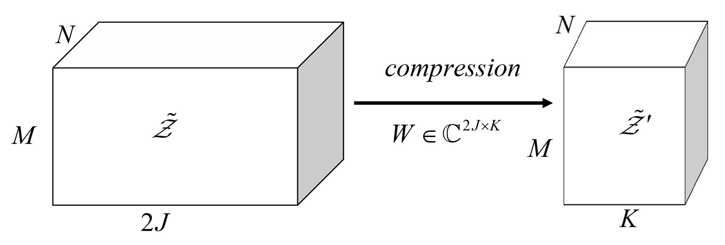
In the process of tensor compression, it is important to obtain a suitable compression matrix. This compression matrix can retain most of the information of the signal, and keep the compressed tensor as small as possible. Principal component analysis (PCA) can retain most of the signal information. Tucker3 decomposition is a higher-order form of PCA [12,27]. The rank of the tensor we obtained is K , K < 2 J , most of the signal information is retained in the first K left singular value vectors. Therefore, the compression matrix can be obtained by truncating Tucker3 decomposition. The tensor compression process is shown in Figure 2, where W takes the first K left singular value vectors after singular value decomposition of Mode-3 unfolding of the tensor Z ¯ . The following is of introduce the details of the compression process:
Firstly, the mode-3 unfolding of the real-valued tensor Z ¯ is:
[ Z ¯ ( 3 ) ] = [ Z ¯ ( 3 ) ] 1 Z ¯ ( 3 ) ] 2 Z ¯ ( 3 ) ] N = A ˜ T D 1 ( A ˜ R ) A ˜ T D 2 ( A ˜ R ) A ˜ T D N ( A ˜ R ) S ˜ T + N ˜ z 1 N ˜ z 2 N ˜ z N = [ A ˜ R A ˜ T ] S ˜ T + N ˜ [ Z ¯ ( 3 ) ]
Then, the compression matrix in the compression process W can be obtained by tucker3 decomposition. The compressed real signal can be expressed as:
[ Z ¯ ( 3 ) ] = [ Z ¯ ( 3 ) ] W = [ A ˜ R A ˜ T ] S ˜ T W + N ˜ [ Z ¯ ( 3 ) ] W = [ A ˜ R A ˜ T ] S ˜ T + N ˜ [ Z ¯ ( 3 ) ]
where W C 2 J × K .
According of the obtained the real-value signal data obtained from Equation (17), the trilinear model can be constructed as follows:
Z ¯ = k = 1 K A ˜ R ( n , k ) A ˜ T ( m , k ) S ˜ ( j , k ) + N ˜ n , m , j n = 1 , , N , m = 1 , , M , j = 1 , , K
The mode-2 unfolding of the real-valued tensor Z ¯ is:
[ Z ¯ ( 2 ) ] = [ A ˜ T S ˜ ] A ˜ R T + N ˜ [ Z ¯ ( 2 ) ]
The mode-1 unfolding of the real-valued tensor Z ¯ is:
[ Z ¯ ( 1 ) ] = [ S ˜ A ˜ R ] A ˜ T T + N ˜ [ Z ¯ ( 1 ) ]

3.3. Trilinear Decomposition

In this section, we estimate the direction matrixs by using the trilinear alternating least square(TALS) method [13].
The LS fitting of Equation (17) is:
min A ˜ R , A ˜ T , S ˜ [ Z ¯ ( 3 ) ] [ A ˜ R A ˜ T ] S ˜ T F
The LS update of S ˜ can be structured as:
S ˜ ^ T = [ A ˜ ^ R A ˜ ^ T ] [ Z ¯ ( 3 ) ]
where A ˜ ^ T is the estimate of A ˜ T and A ˜ ^ R is the estimate of A ˜ R .
The LS fitting of Equation (19) is:
min A ˜ R , A ˜ T , S ˜ [ Z ¯ ( 2 ) ] [ A ˜ T S ˜ ] A ˜ R T F
The LS update of A ˜ R is:
A ˜ ^ R T = [ A ˜ ^ T S ˜ ^ ] [ Z ¯ ( 2 ) ]
where S ˜ ^ is the estimate of S ˜ and A ˜ ^ T is the estimate of A ˜ T .
The least square (LS) fitting of Equation (20) is:
min A ˜ R , A ˜ T , S ˜ [ Z ¯ ( 1 ) ] [ S ˜ A ˜ R ] A ˜ T T F
The LS update of A ˜ T is:
A ˜ ^ T T = [ S ˜ ^ A ˜ ^ R ] [ Z ¯ ( 1 ) ]
where A ˜ ^ R is the estimate of A ˜ R and S ˜ ^ is the estimate of S ˜ .
According to Equations (22), (24) and (26), the matrices A ˜ T , S ˜ and A ˜ R are updated cyclically until convergence, where the convergence condition is [ Z ¯ ( 3 ) ] [ A ˜ ^ R A ˜ ^ T ] S ˜ ^ T F 2 10 10 .
After trilinear decomposition, the estimation of the three factor matrices satisfies: A ˜ ^ R = A ˜ R Γ Δ 1 + N 1 , A ˜ ^ T = A ˜ T Γ Δ 2 + N 2 , S ˜ ^ = S ˜ Γ Δ 3 + N 3 . Where Γ stand for a permutation matrix, N 1 , N 2 , N 3 are estimation errors, Δ 1 , Δ 2 , Δ 3 denote the diagonal scaling matrices, and the product of these three matrices satisfies Δ 1 Δ 2 Δ 3 = I .

3.4. Range and Angle Estimation

In the previous section, the estimation of the direction matrices A ˜ ^ T and A ˜ ^ R has been obtained by the LS method. According to U N U N H = I and U M U M H = I , we obtain the following formula:
h r = a n g l e ( U N A ˜ R ) = [ 1 , 2 d λ π sin θ k , , ( N 1 ) 2 d λ π sin θ k ] T
h t = a n g l e ( U M A ˜ T ) = [ 1 , 2 d λ π ( sin θ k 4 Δ f r k c ) , , ( M 1 ) 2 d λ π ( sin θ k 4 Δ f r k c ) ] T
Define
G r = 1 0 1 2 d λ π 1 2 ( N 1 ) d λ π
G t = 1 0 1 2 d λ π 1 2 ( M 1 ) d λ π
Then, the estimation of sin θ k and ( sin θ k 4 Δ f r k c ) can be obtained by using LS method. LS fitting can be constructed as:
G r v r = h r
G t v t = h t
where v r C 2 × 1 and v t C 2 × 1 are the estimated vectors.
The LS solutions of v r and v t are:
v ^ r = ( G r T G r ) 1 G r T h ^ r
v ^ t = ( G t T G t ) 1 G t T h ^ t
The estimation of angle can be obtained from the following formula:
θ ^ k = arcsin ( v ^ r ( 2 ) )
where v ^ r ( 2 ) stand for the second element of vector v ^ r .
The estimation of range can be obtained from the following formula:
r ^ k = v ^ r ( 2 ) v ^ t ( 2 ) 4 Δ f × c
where v ^ t ( 2 ) stand for the second element of vector v ^ t .

3.5. Complexity Analysis and Cramer-Rao Bound

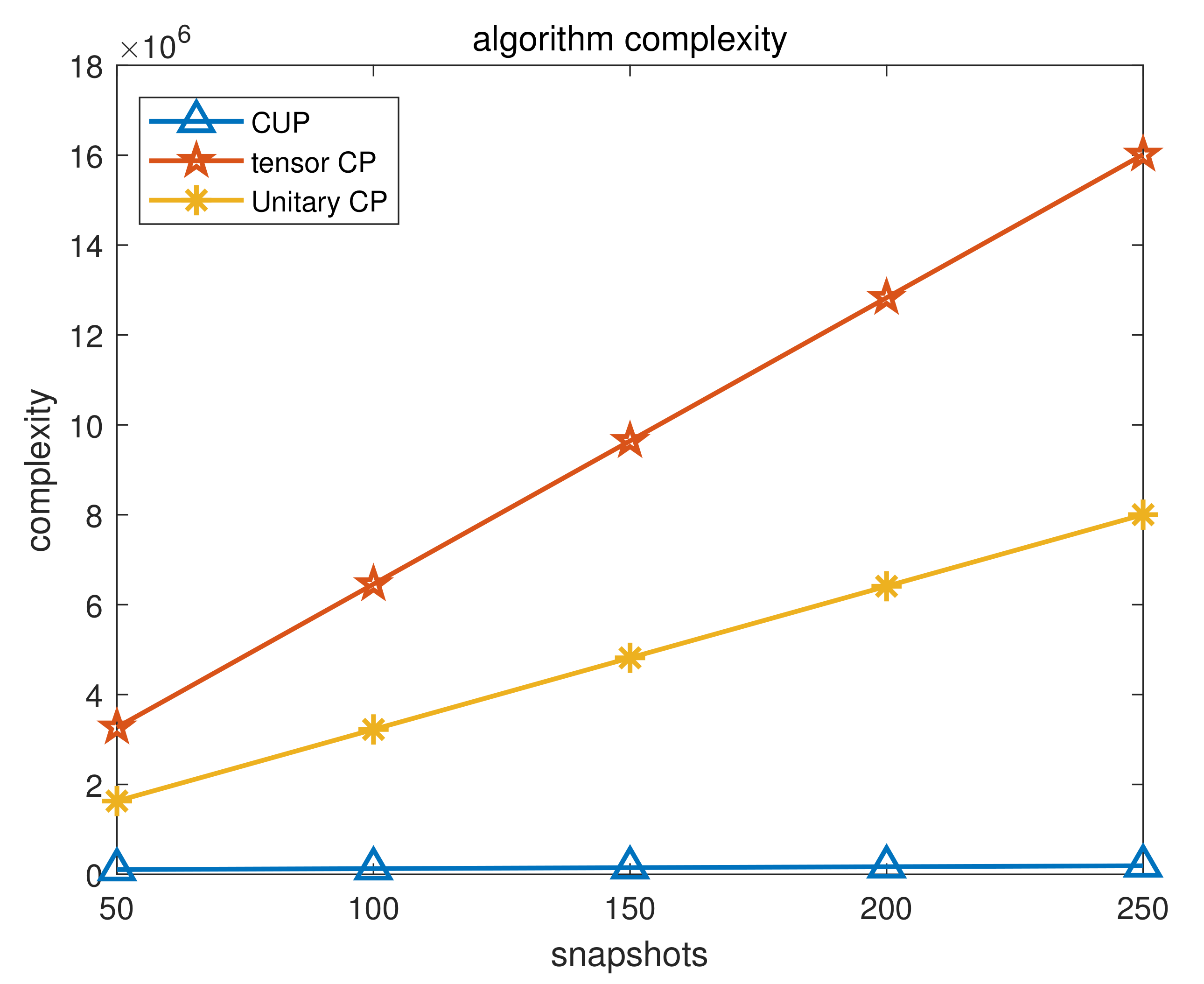
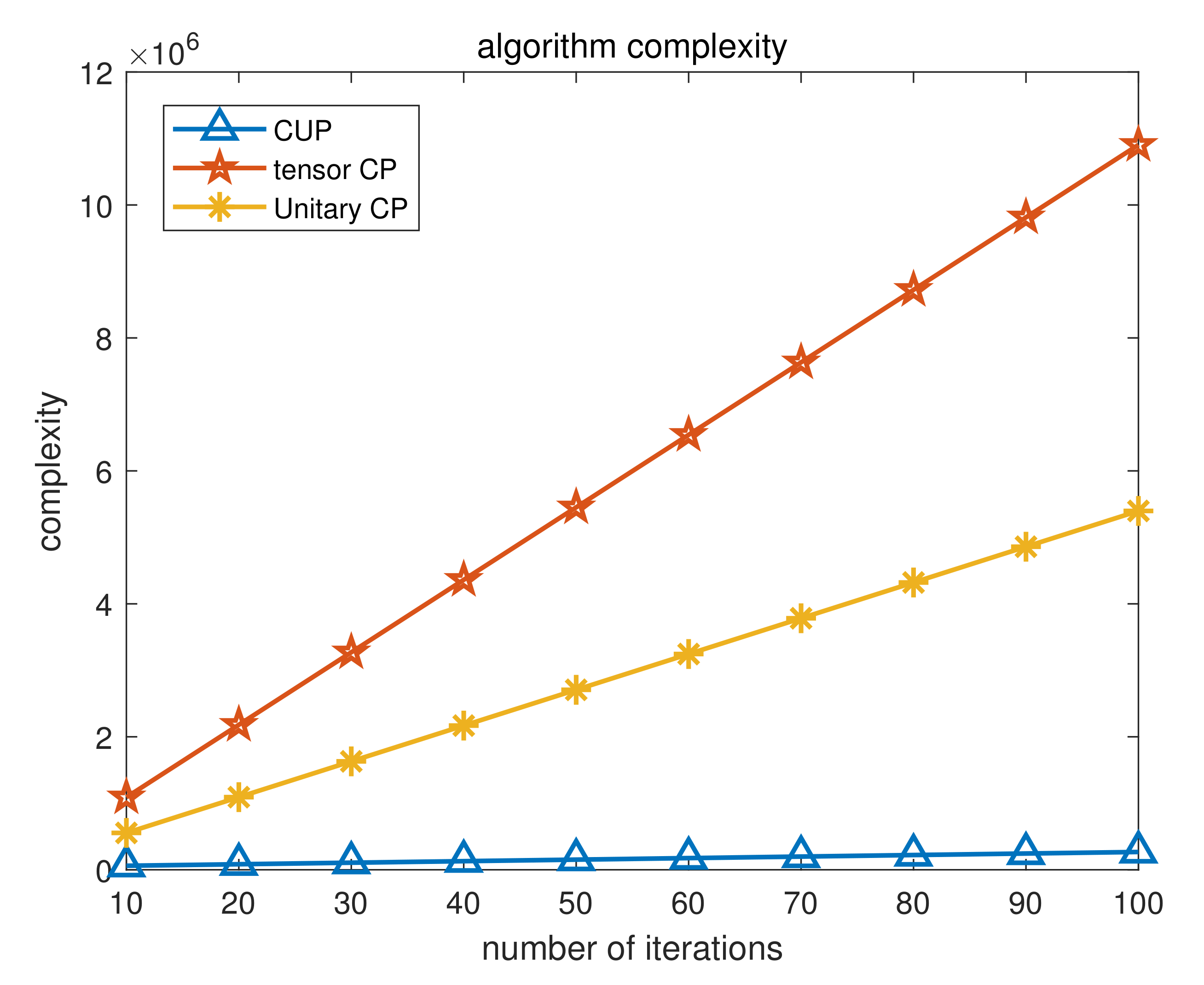
In the paper, the total complexity of the forward–backward process and unitary transformation process in the CUP is O ( 8 M K N 2 + 8 M 2 K N + 20 M K 2 N ) . The complexity of the compression process in the CUP is O ( 4 M N J K ) . The complexity of each iteration process of TALS in the CUP, the traditional PARAFAC method and the unitary PARAFAC method are O ( 2 K 2 ( M N + M K + N K ) + 3 K 2 M N + 3 K 3 ) , O ( 8 K 2 ( M N + M J + N J ) + 12 K M N J + 12 K 3 ) and O ( 2 K 2 ( M N + 2 M J + 2 N J ) + 6 K M N J + 12 K 3 ) , respectively. Therefore, the complexity of the CUP is O ( 8 M K N 2 + 8 M 2 K N + 20 M K 2 N + 4 M N J K + n 1 ( 2 K 2 ( M N + M K + N K ) + 3 K 2 M N + 3 K 2 ) ) , the complexity of the traditional PARAFAC method is O ( n 2 ( 8 K 2 ( M N + M J + N J ) + 12 K M N J + 12 K 3 ) ) , the complexity of the unitary PARAFAC method is O ( 8 M K N 2 + 8 M 2 K N + 20 M K 2 N + n 3 ( 2 K 2 ( M N + 2 M J + 2 N J ) + 6 K M N J + 3 K 3 ) ) , where n 1 n 2 and n 3 are the number of the CUP, the traditional PARAFAC method and the unitary PARAFAC method, respectively. In order to more clearly compare the complexity of the three methods and the relationship between their computational complexity and the number of snapshots, we assume M = 5 , N = 7 , K = 3 , n 1 = n 2 = n 3 = 30 . From Figure 3, with the increase of the number of snapshots, the difference of the complexity of the three methods becomes more and more obvious. Then, we also analyze the relationship between the complexity of the three methods and the number of iterations. We set M = 5 , N = 7 , K = 3 , J = 50 . It can be easily found from Figure 4 that the increase of the number of iterations will increase the complexity gap between the three algorithms. Through complexity analysis, it can be concluded that the complexity of the PARAFAC-based method is hugely reduced after the real value transformation and compression of the tensor.
According to [28], the Cramer–Rao Bound (CRB) for FDA-MIMO range and angle estimation is as follows:
C R B = σ 2 2 J { R e [ D H B 1 A D P T ] } 1
where D = [ ( ( a ( θ 1 , r 1 ) ) / θ 1 ) , , ( ( a ( θ 1 , r 1 ) ) / r 1 ) , ] , B 1 A = I M N A ( A H A ) 1 A H , P = [ P 1 P 1 ; P 1 P 1 ] , where P 1 = S S H / J .

4. Simulation Results

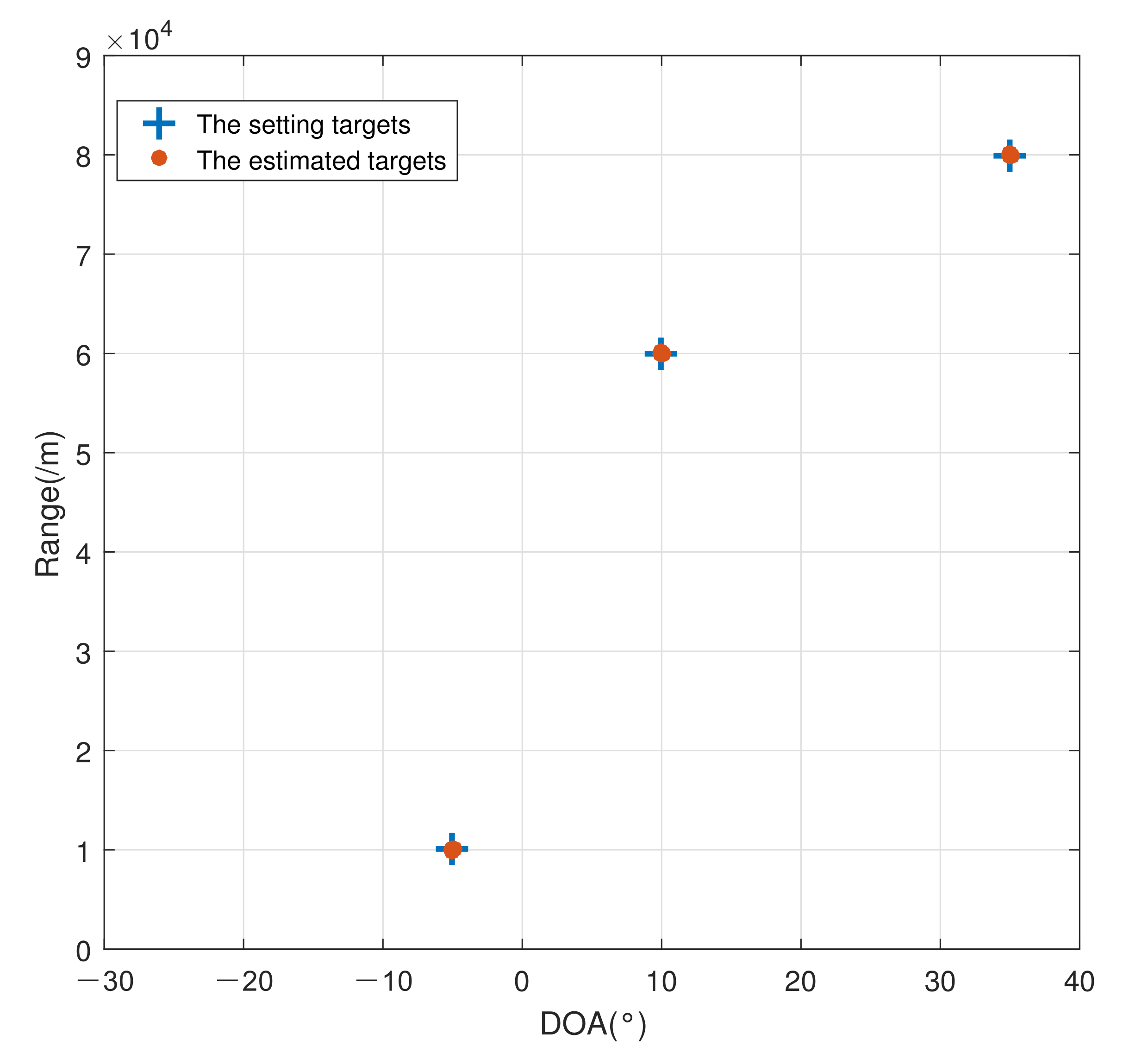
In this section, we conducted several experiments to verify the superiority and effectiveness of the CUP. At the same time, we compared the CUP with the ESPRIT method [22], the unitary ESPRIT method [24], the traditional PARAFAC method [23], the unitary PARAFAC method. In the following experiment, the total number of transmitting arrays of FDA-MIMO is M = 5 , and the total number of receiving arrays is N = 7 . The total number of uncorrelated targets is K = 3 in the following simulation experiment. The angle and range of these targets are: ( θ 1 , r 1 ) = ( 5 , 10 km), ( θ 2 , r 2 ) = ( 10 , 60 km), and ( θ 3 , r 3 ) = ( 35 , 80 km). The number of Monte Carlo in the simulation experiment is set of Q = 500 . This paper used the Root Square Mean Error (RMSE) compare the performance of these algorithms. The RMSE of the range estimate and angle estimate are:
RMSE r = 1 K 1 Q k = 1 K q = 1 Q ( r ^ k , q r k ) 2
RMSE θ = 1 K 1 Q k = 1 K q = 1 Q ( θ ^ k , q θ k ) 2
where r ^ k , q and θ ^ k , q are the estimated range and angle of k-th target in q-th Monte Carlo experiment, respectively.
We assume that the estimation error of all angles is less than 0 . 1 , this time the angle estimation can be considered successful, and the range estimation can only be considered successful when all the range estimation errors are less than 0.2 km. The expression of the probability of the successful detection (PSD) is:
PSD r = D r Q × 100 %
PSD θ = D θ Q × 100 %
where D r and D θ are the number of successful estimates of range and angle, respectively.

4.1. Stability Simulation

In this experiment, the signal-to-noise ratio (SNR) is S N R = 20 , the total number of snapshots is J = 50 . It can be easily seen from Figure 5 that the estimated range and angle values in the 20 experiments are all around the set values. Additionally, the errors that can be found in Table 2 are all between ± 0.2 km and ± 0 . 1 , which proves that the angle and range of the target are accurately estimated by the CUP. This experiment reflects the effectiveness and stability of the CUP.

4.2. Simulation of Algorithm Performance with RMSE Changing with SNR

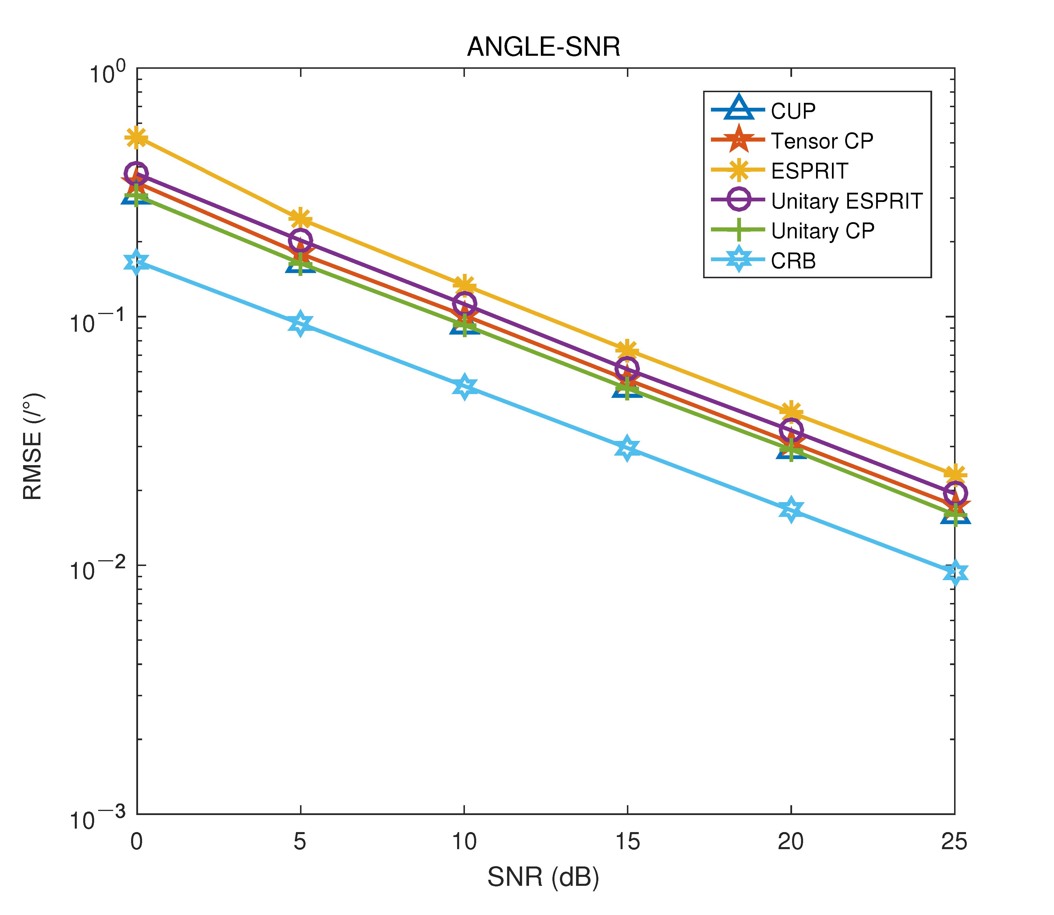
In this experiment, the total number of snapshots is J = 50 . Figure 6 and Figure 7 show that the RMSE curves of the CUP are consistently lower than those of the traditional PARAFAC method [23], the unitary ESPRIT method [24], and the ESPRIT method [22], and are close to those of the unitary PARAFAC method. Moreover, these curves fall as SNR rises. More specifically, as shown in Table 3 and Table 4, the RMSE values of the CUP are smaller than those of the ESPRIT method, the unitary ESPRIT method, and the traditional PARAFAC method; the RMSE values of the CUP are almost close to the RMSE values of the unitary PARAFAC method, in which the differences of the angle RMSE value of the two algorithms do not exceed 0 . 0005 and the differences of the range RMSE values of the two algorithms do not exceed 0.0004 km. Furthermore, the RMSE values decrease with increasing SNR. The smaller the RMSE, the better the estimated performance. Therefore, from these figures and tables, we find that the estimation performance of the CUP outperforms the ESPRIT method, the unitary ESPRIT method, and the traditional PARAFAC method, and is close to the unitary PARAFAC method. The reason for why the performance of the CUP is close to the unitary PARAFAC method is that the compression matrix obtained by TUCKER3 decomposition during tensor compression contains most of the information of the signal. Moreover, we can also find that the estimation performance of these algorithms improves as the SNR increases.

4.3. Simulation of Algorithm Performance with RMSE Changing with Snapshots

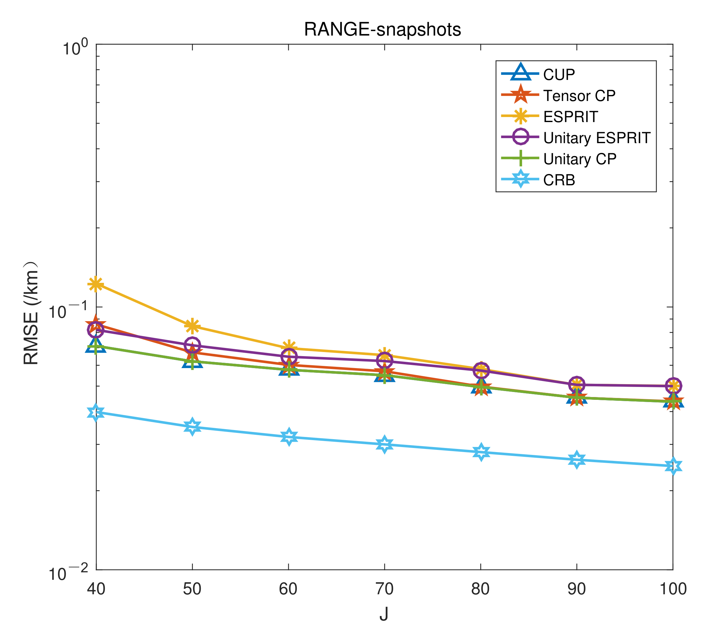
In this experiment, the SNR is 20. It can be seen from Figure 8 and Figure 9 that the RMSE curves of the CUP are lower than those of the traditional PARAFAC method when the number of snapshots is less than 80 and coincides with those of the traditional PARAFAC method when the number of snapshots is more than 80; the RMSE curves of the CUP are always lower than those of the ESPRIT method, the unitary ESPRIT method, and always coincides with the RMSE curve of the unitary PARAFAC method. Furthermore, the RMSE curves of these algorithms all decrease as the number of snapshots increases. More obviously, it can be found from Table 5 and Table 6 that when the number of snapshots is less than 80, the RMSE values of the CUP are lower than those of the traditional PARAFAC method, and when the number of snapshots is greater than 80, they are equal of those of the traditional PARAFAC; the RMSE values of the CUP are always less than those of the ESPRIT method, the unitary ESPRIT method, and are always the same as those of the unitary PARAFAC method. Furthermore, the RMSE values of these algorithms reduce with the increase of the number of snapshots. Consequently, from these figures and tables, we find that the estimated performance of the algorithm improves as the number of snapshots increases, and the CUP performance is better than the traditional PARAFAC algorithm in the case of low snapshots. The reason for this is that the CUP increases the number of virtual snapshots of the algorithm by the forwards–backwards technique.

4.4. Simulation of Algorithm Performance with PSD Changing with SNR

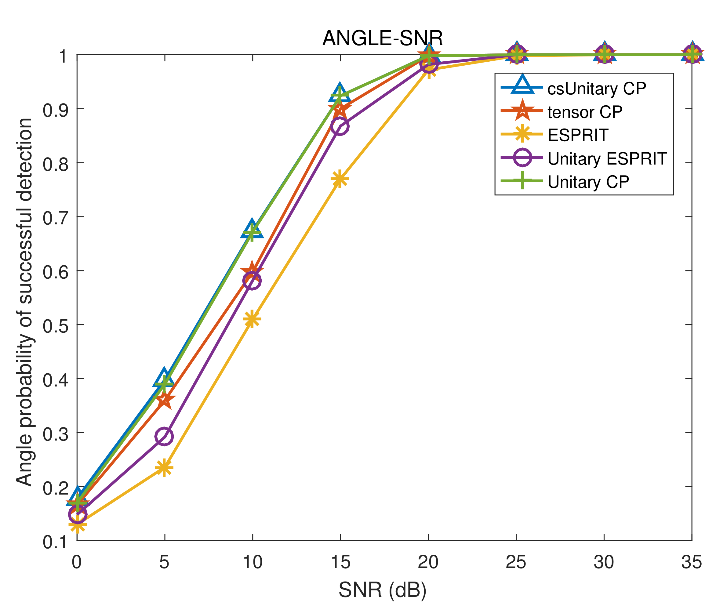
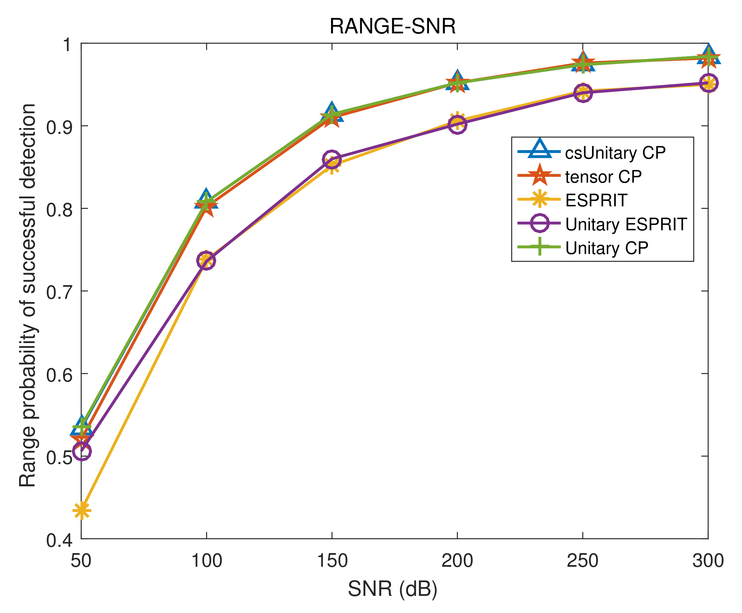
In this experiment, the total number of snapshots is J = 50 . From Figure 10 and Figure 11, we find that the PSD curves of the CUP are higher than those of the traditional PARAFAC method [23], the unitary ESPRIT method [24], and the ESPRIT method [22]; the PSD curves of the CUP are close of those of the unitary PARAFAC method. Additionally, these PSD curves rise with the increase of SNR and finally reach PSD = 1. More clearly, it can be seen from Table 7 and Table 8 that the PSD values of the CUP and the unitary PARAFAC method are close, and the differences between the PSD values of the two methods are no more than 0.5 % ; The PSD values of the CUP are higher than those of the traditional PARAFAC method, the ESPRIT method, and the unitary ESPRIT method. Moreover, the PSD values of all algorithms increase with the rise of SNR, and the final PSD values reach 100 % . The angle PSD value of the CUP reaches 100 % when the SNR is 20, that of the unitary ESPRIT method and the traditional PARAFAC method reaches 100 % when the SNR is 25, and that of the ESPRIT method reaches 100 % when the SNR is 30. The higher the PSD value, the better the estimation performance of the algorithm. Thus, in these figures and tables, we find that the estimation performance of the CUP is better than the ESPRIT method, the unitary ESPRIT method, and the traditional PARAFAC method and is close to the unitary PARAFAC method.

4.5. Simulation of Algorithm Performance with PSD Changing with Snapshots

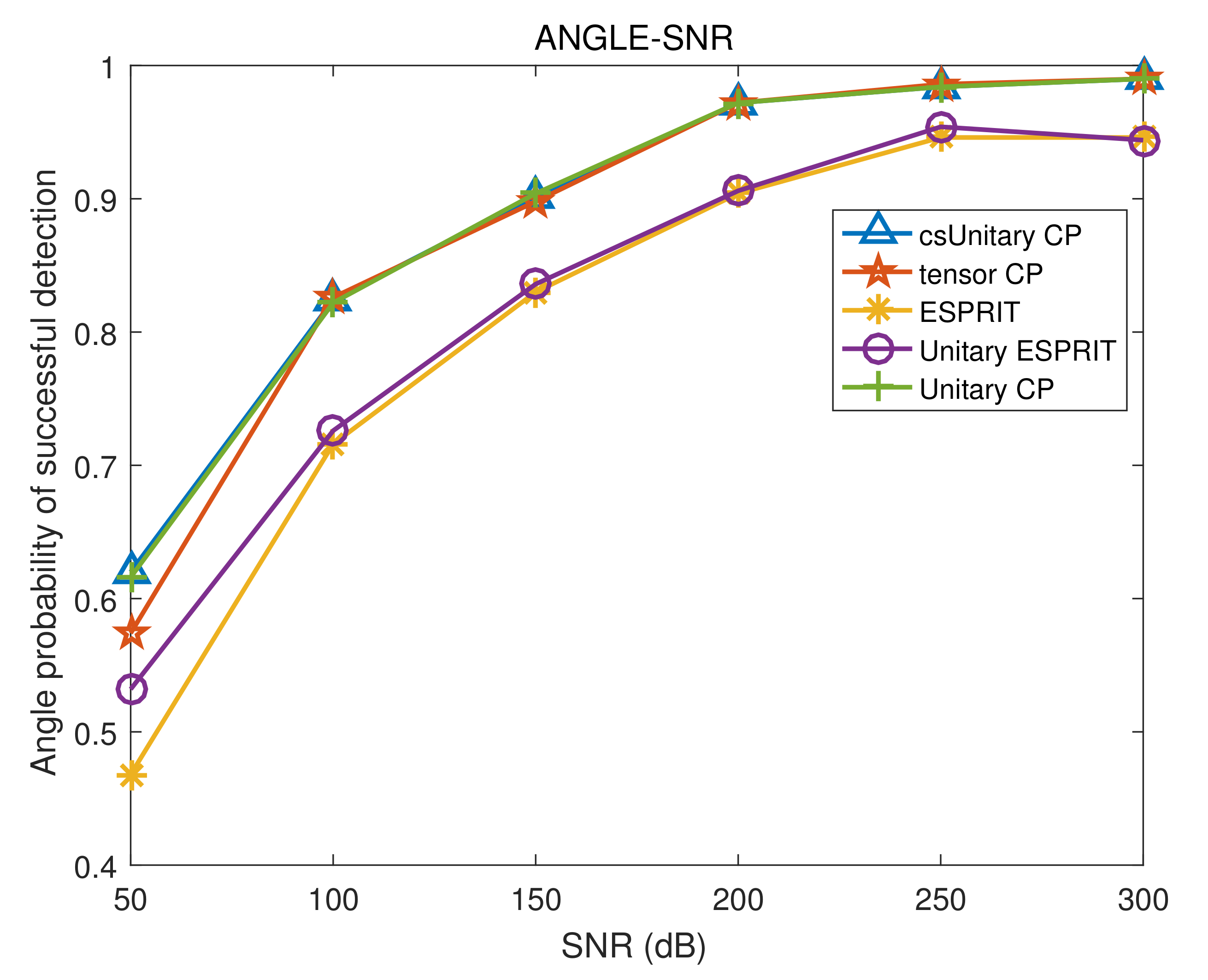
In this experiment, the SNR is 10. It can be seen from Figure 12 and Figure 13 that the PSD curves of the CUP are significantly higher than those of the traditional PARAFAC method [23] when the number of snapshots is 50 and are close to those of the traditional PARAFAC method when the number of snapshots is greater than 100; the PSD curves of the CUP are higher than the ESPRIT method [22] and the unitary ESPRIT method [24] and coincide with the PSD curves of the unitary PARAFAC method. These PSD curves increase with the increase of the number of snapshots. More obviously, as shown in Table 9 and Table 10, the PSD values of the CUP are higher than those of the ESPRIT method and the unitary ESPRIT method; the PSD values of the CUP are close to those of the unitary PARAFAC method, and the differences of the PSD values of the two methods are no more than 0.4 % ; when the number of snapshots is 50, the angle PSD values of the CUP are 4.8 % higher than that of the traditional PARAFAC method and the range PSD value of the CUP is 3 % higher than that of the traditional PARAFAC method; the difference between the PSD value of the CUP and the traditional PARAFAC method does not exceed 0.6 % when the number of snapshots exceeds 100. The PSD values of these algorithms increase with the improvement of the number of snapshots. Therefore, we can find from these figures and tables that the CUP has better performance than the traditional PARAFAC method when the number of snapshots is low and a close performance when the number of snapshots is high.

5. Conclusions

In the paper, a joint range and angle estimation method based on compressed unitary PARAFAC decomposition in monostatic FDA-MIMO radar was proposed. In CUP, a third-order real-valued signal tensor with twice the number of samples is constructed by utilizing a forward–backward technique and unitary transformation technique. Afterward, the compression matrix is used to compress the third-order real-valued signal tensor to form a smaller third-order real-valued signal tensor. This compressed matrix is obtained by truncated TUCKER3 decomposition. Next, we estimate the direction matrices by the TALS method. Finally, the estimated range and angle are obtained by extracting the range and angle information in the direction matrix. The CUP uses forward–backward technology of improve the number of samples. Compared with the traditional PARAFAC method, the CUP can estimate more accurate angles and ranges when the number of snapshots is small, especially when the SNR is low. For example, when the SNR is 0 and the number of snapshots is 50, the angle error and range error of the CUP are 9.9 % and 10.5 % lower than those of the traditional PARAFAC algorithm, respectively. Furthermore, the third-order real-valued tensor and compression technology are constructed by unitary transformation of reduce the complexity of the method. When the number of snapshots is as low as 50 and the number of iterations is 30, the complexity of the CUP is 96.7 % lower than that of the traditional PARAFAC algorithm. The difference between the complexity of the two algorithms is more pronounced at higher snapshots and more iterations.

Author Contributions

Conceptualization, W.W. and X.W.; methodology, W.W. and X.W.; writing—original draft preparation, W.W.; writing—review and editing, X.W. and X.L.; supervision, X.W.; funding acquisition, X.W. and J.S. All authors have read and agreed of the published version of the manuscript.

Funding

This work was supported by Key Research and Development Program of Hainan Province (No. ZDYF2020019), the National Natural Science Foundation of China (No.61861015, 61961013,62101165), National Key Research and Development Program of China(No. 2019CXTD400, No.SQ2020YFF0405680), Young Elite Scientists Sponsorship Program by CAST (No.2018QNRC001).

Institutional Review Board Statement

Not applicable.

Informed Consent Statement

Not applicable.

Data Availability Statement

Not applicable.

Conflicts of Interest

The authors declare no conflict of interest.

References

  1. Coluccia, A.; Fascista, A.; Ricci, G. CFAR feature plane: A novel framework for the analysis and design of radar detectors. IEEE Trans. Signal Process. 2020, 68, 3903–3916. [Google Scholar] [CrossRef]
  2. Cao, Z.; Fang, W.; Song, Y.; He, L.; Song, C.; Xu, Z. DNN-Based Peak Sequence Classification CFAR Detection Algorithm for High-Resolution FMCW Radar. IEEE Trans. Geosci. Remote. Sens. 2021, 60, 1–15. [Google Scholar] [CrossRef]
  3. Rabideau, D.J.; Parker, P. Ubiquitous MIMO multifunction digital array radar. In Proceedings of the Thrity-Seventh Asilomar Conference on Signals, Systems & Computers, Pacific Grove, CA, USA, 9–12 November 2003; pp. 1057–1064. [Google Scholar]
  4. Fishler, E.; Haimovich, A.; Blum, R.; Chizhik, D.; Cimini, L.; Valenzuela, R. MIMO radar: An idea whose time has come. In Proceedings of the 2004 IEEE Radar Conference (IEEE Cat. No. 04CH37509), Philadelphia, PA, USA, 29–29 April 2004; pp. 71–78. [Google Scholar]
  5. Bliss, D.W.; Forsythe, K.W. Multiple-input multiple-output (MIMO) radar and imaging: Degrees of freedom and resolution. In Proceedings of the Thrity-Seventh Asilomar Conference on Signals, Systems & Computers, Pacific Grove, CA, USA, 9–12 November 2003; pp. 54–59. [Google Scholar]
  6. Wang, X.; Yang, L.T.; Meng, D.; Dong, M.; Ota, K.; Wang, H. Multi-UAV cooperative localization for marine targets based on weighted subspace fitting in SAGIN environment. IEEE Internet Things J. 2021, in press. [Google Scholar] [CrossRef]
  7. Antonik, P.; Wicks, M.C.; Griffiths, H.D.; Baker, C.J. Frequency diverse array radars. In Proceedings of the 2006 IEEE Conference on Radar, Verona, NY, USA, 24–27 April 2006; p. 3. [Google Scholar]
  8. Wang, W.Q. Subarray-based frequency diverse array radar for target range-angle estimation. IEEE Trans. Aerosp. Electron. Syst. 2014, 50, 3057–3067. [Google Scholar] [CrossRef]
  9. Chen, H.; Shao, H.Z. Sparse reconstruction based target localization with frequency diverse array MIMO radar. In Proceedings of the 2015 IEEE China Summit and International Conference on Signal and Information Processing (ChinaSIP), Chengdu, China, 12–15 July 2015; pp. 94–98. [Google Scholar]
  10. Xu, J.; Liao, G.; Zhang, Y.; Ji, H.; Huang, L. An adaptive range-angle-Doppler processing approach for FDA-MIMO radar using three-dimensional localization. IEEE J. Sel. Top. Signal Process 2016, 11, 309–320. [Google Scholar] [CrossRef]
  11. Xu, J.; Wang, W.Q.; Cui, C.; Gui, R. Joint range, angle and doppler estimation for FDA-MIMO radar. In Proceedings of the 2018 IEEE 10th Sensor Array and Multichannel Signal Processing Workshop (SAM), Sheffield, UK, 8–11 July 2018; pp. 499–503. [Google Scholar]
  12. Kolda, T.G.; Bader, B.W. Tensor decompositions and applications. SIAM Rev. 2009, 51, 455–500. [Google Scholar] [CrossRef]
  13. Zhang, X.; Xu, Z.; Xu, L.; Xu, D. Trilinear decomposition-based transmit angle and receive angle estimation for multiple-input multiple-output radar. IET Radar Sonar Navig. 2011, 5, 626–631. [Google Scholar] [CrossRef]
  14. Xu, B.; Zhao, Y.; Cheng, Z.; Li, H. A novel unitary PARAFAC method for DOD and DOA estimation in bistatic MIMO radar. Signal Process. 2017, 138, 273–279. [Google Scholar] [CrossRef]
  15. Xu, L.; Wen, F.; Zhangm, X. A novel unitary PARAFAC algorithm for joint DOA and frequency estimation. IEEE Commun. Lett. 2019, 23, 660–663. [Google Scholar] [CrossRef]
  16. Xu, B.; Zhao, Y. Transmit beamspace-based unitary parallel factor method for DOD and DOA estimation in bistatic MIMO radar. IEEE Access 2018, 6, 65573–65581. [Google Scholar] [CrossRef]
  17. Xu, L.; Wu, R.; Zhang, X.; Shi, Z. Joint two-dimensional DOA and frequency estimation for L-shaped array via compressed sensing PARAFAC method. IEEE Access 2018, 6, 37204–37213. [Google Scholar] [CrossRef]
  18. Li, S.; Sun, Z.; Zhang, X.; Chen, W.; Xu, D. Joint DOA and frequency estimation for linear array with compressed sensing PARAFAC framework. J. Circuits Syst. Comput. 2017, 26, 1750136. [Google Scholar] [CrossRef]
  19. Cao, R.; Zhang, X.; Chen, W. Compressed sensing parallel factor analysis-based joint angle and Doppler frequency estimation for monostatic multiple-input–multiple-output radar. IET Radar Sonar Navig. 2014, 8, 597–606. [Google Scholar] [CrossRef]
  20. Li, S.; Zhang, X.F. Study on the compressed matrices in compressed sensing trilinear model. Appl. Mech. Mater. 2014, 556, 3380–3383. [Google Scholar] [CrossRef]
  21. Sidiropoulos, N.D.; Kyrillidis, A. Multi-way compressed sensing for sparse low-rank tensors. IEEE Signal Process. Lett. 2012, 19, 757–760. [Google Scholar] [CrossRef] [Green Version]
  22. Li, B.; Bai, W.; Zheng, G. Successive ESPRIT algorithm for joint DOA-range-polarization estimation with polarization sensitive FDA-MIMO radar. IEEE Access 2018, 6, 36376–36382. [Google Scholar] [CrossRef]
  23. Xu, T.; Yang, Y.; Huang, M.; Wang, H.; Wu, D.; Yi, Q. Tensor-based angle and range estimation method in monostatic FDA-MIMO radar. Math. Probl. Eng. 2020, 2020, 5720189. [Google Scholar] [CrossRef]
  24. Liu, F.; Wang, X.; Huang, M.; Wan, L.; Wang, H.; Zhang, B. A novel unitary ESPRIT algorithm for monostatic FDA-MIMO radar. Sensors 2020, 20, 827. [Google Scholar] [CrossRef] [Green Version]
  25. Haardt, M.; Roemer, F.; Del Galdo, G. Higher-order SVD-based subspace estimation of improve the parameter estimation accuracy in multidimensional harmonic retrieval problems. IEEE Trans. Signal Process. 2008, 56, 3198–3213. [Google Scholar] [CrossRef]
  26. Wang, X.; Wang, W.; Liu, J.; Liu, Q.; Wang, B. Tensor-based real-valued subspace approach for angle estimation in bistatic MIMO radar with unknown mutual coupling. Signal Process. 2015, 116, 152–158. [Google Scholar] [CrossRef]
  27. Andersson, C.A.; Bro, R. Improving the speed of multi-way algorithms: Part I. Tucker3. Chemom. Intell. Lab. Syst. 1998, 42, 93–103. [Google Scholar] [CrossRef]
  28. Xiong, J.; Wang, W.Q.; Gao, K. FDA-MIMO radar range-angle estimation: CRLB, MSE, and resolution analysis. IEEE Trans. Aerosp. Electron. Syst. 2017, 54, 284–294. [Google Scholar] [CrossRef]
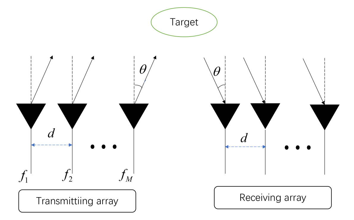
Figure 1. Monostatic FDA-MIMO radar model.
Remotesensing 14 01398 g001
Figure 2. Tensor compression process.
Remotesensing 14 01398 g002
Figure 3. Complexity comparison and snapshots.
Remotesensing 14 01398 g003
Figure 4. Complexity comparison and iterations.
Remotesensing 14 01398 g004
Figure 5. The estimated result of the method with S N R = 20 dB, J = 50 .
Remotesensing 14 01398 g005
Figure 6. RMSE of angle estimation versus SNR.
Remotesensing 14 01398 g006
Figure 7. RMSE of range estimation versus SNR.
Remotesensing 14 01398 g007
Figure 8. RMSE of angle estimation versus snapshots.
Remotesensing 14 01398 g008
Figure 9. RMSE of range estimation versus snapshots.
Remotesensing 14 01398 g009
Figure 10. PSD of angle estimation versus SNR.
Remotesensing 14 01398 g010
Figure 11. PSD of range estimation versus SNR.
Remotesensing 14 01398 g011
Figure 12. PSD of angle estimation versus Snapshots.
Remotesensing 14 01398 g012
Figure 13. PSD of range estimation versus Snapshots.
Remotesensing 14 01398 g013
Table 1. Related notation.
NotationsDefinitions
( · ) H conjugate-transpose
( · ) T transpose
( · ) conjugate
( · ) pseudo-inverse
( · ) 1 inverse
Khatri–Rao product operator
Kronecker product operator
  ·   the Frobenius norm operator
D n ( A ) the diagonal matrix composed of the n-th row of  A .
R e ( · ) the real part operator
identity matrix the vector outer product operator
I K K × K identity matrix
Table 2. Stability Simulation.
Targets 5 10 km 10 60 km 35 80 km
Time
1 4 . 9914 9.9723 km 10 . 0366 59.9731 km 35 . 0131 80.0439 km
2 5 . 0199 9.9351 km 10 . 0096 60.0551 km 34 . 9797 79.8586 km
3 4 . 9731 9.9519 km 10 . 0136 60.0696 km 35 . 0297 80.0381 km
4 4 . 9662 10.0124 km 9 . 9996 60.0360 km 35 . 0163 80.0233 km
5 4 . 9796 10.0312 km 9 . 9729 59.9638 km 35 . 0041 79.9552 km
6 5 . 0081 10.0845 km 10 . 0213 60.0429 km 35 . 0121 80.0241 km
7 4 . 9525 10.0540 km 9 . 9736 59.9131 km 35 . 0021 80.0894 km
8 5 . 0093 9.9456 km 10 . 0001 59.9563 km 35 . 0174 80.0051 km
9 5 . 0098 9.9662 km 9 . 9714 59.9421 km 35 . 0456 80.0094 km
10 5 . 0138 10.0045 km 9 . 9844 59.9912 km 35 . 0175 79.9996 km
11 4 . 9733 10.0388 km 10 . 0153 60.0276 km 35 . 0032 79.9188 km
12 4 . 9965 9.9522 km 9 . 9881 60.0585 km 35 . 0089 79 , 9730 km
13 4 . 9902 9.9782 km 9 . 9800 59.9519 km 34 . 9850 80.0346 km
14 5 . 0038 9.9585 km 10 . 0074 60.1063 km 34 . 9486 79.9092 km
15 5 . 0055 9.9592 km 9 . 9813 60.0371 km 35 . 0352 80.0866 km
16 4 . 9601 10.0271 km 10 . 0366 60.0561 km 35 . 0168 80.0513 km
17 5 . 0313 9.9330 km 9 . 9364 59.8802 km 35 . 0000 79.9561 km
18 5 . 0045 10.0191 km 10 . 0133 59.9373 km 35 . 0717 79.9803 km
19 5 . 0149 9.9883 km 10 . 0226 60.0302 km 35 . 0415 80.0243 km
20 5 . 0107 10.0541 km 10 . 0449 60.0603 km 34 . 9914 80.9997 km
Table 3. RSME of angle estimation versus SNR.
AlgorithmSNR = 0SNR = 5SNR = 10SNR = 15SNR = 20SNR = 25
CRB 0 . 1664 0 . 0936 0 . 0526 0 . 0296 0 . 0166 0 . 0094
CUP 0 . 2984 0 . 1620 0 . 0929 0 . 0528 0 . 0289 0 . 0162
unitary CP 0 . 2979 0 . 1619 0 . 0929 0 . 0528 0 . 0289 0 . 0162
tensor CP 0 . 3312 0 . 1761 0 . 1022 0 . 0572 0 . 0318 0 . 0179
unitary ESPRIT 0 . 3789 0 . 1960 0 . 1098 0 . 0614 0 . 0355 0 . 0194
ESPRIT 0 . 5202 0 . 2444 0 . 1329 0 . 0736 0 . 0426 0 . 0231
Table 4. RSME of range estimation versus SNR.
Algorithm (km)SNR = 0SNR = 5SNR = 10SNR = 15SNR = 20SNR = 25
CRB (km) 0.3495 0.1965 0.1105 0.0621 0.0349 0.0197
CUP (km) 0.6365 0.3559 0.1992 0.1140 0.0612 0.0348
unitary CP (km) 0.6361 0.3559 0.1992 0.1140 0.0612 0.0348
tensor CP (km) 0.7113 0.3973 0.2205 0.1216 0.0663 0.0379
unitary ESPRIT (km) 0.7249 0.4091 0.2251 0.1270 0.0714 0.0393
ESPRIT (km) 1.0331 0.5196 0.2680 0.1544 0.0853 0.0489
Table 5. RSME of angle estimation versus Snapshots.
AlgorithmJ = 40J = 50J = 60J = 70J = 80J = 90J = 100
CRB 0 . 0190 0 . 0166 0 . 0152 0 . 0143 0 . 0133 0 . 0125 0 . 0118
CUP 0 . 0335 0 . 0281 0 . 0258 0 . 0247 0 . 0230 0 . 0211 0 . 0200
unitary CP 0 . 0335 0 . 0281 0 . 0258 0 . 0247 0 . 0230 0 . 0211 0 . 0200
tensor CP 0 . 0404 0 . 0306 0 . 0269 0 . 0251 0 . 0230 0 . 0211 0 . 0200
unitary ESPRIT 0 . 0410 0 . 0335 0 . 0313 0 . 0297 0 . 0284 0 . 0260 0 . 0241
ESPRIT 0 . 0589 0 . 0398 0 . 0346 0 . 0311 0 . 0286 0 . 0260 0 . 0242
Table 6. RSME of range estimation versus Snapshots.
AlgorithmJ = 40J = 50J = 60J = 70J = 80J = 90J = 100
CRB (km) 0.0398 0.0349 0.0320 0.0300 0.0280 0.0262 0.0248
CUP (km) 0.0717 0.0613 0.0552 0.0529 0.0513 0.0475 0.0439
unitary CP (km) 0.0717 0.0613 0.0552 0.0529 0.0513 0.0475 0.0439
tensor CP (km) 0.0860 0.0662 0.0573 0.0543 0.0515 0.0473 0.0440
unitary ESPRIT (km) 0.0818 0.0690 0.0624 0.0624 0.0604 0.0544 0.0501
ESPRIT (km) 0.1238 0.0828 0.0696 0.0657 0.0610 0.0545 0.0502
Table 7. PSD of angle estimation versus SNR.
AlgorithmSNR = 0SNR = 5SNR = 10SNR = 15SNR = 20SNR = 25SNR = 30
CUP20.2%40.6%63.2%92.3%100%100%100%
unitary CP20.6%41.0%63.4%92.4%100%100%100%
tensor CP18.6%34.8%59.0%90.6%99.6%100%100%
unitary ESPRIT16.6%30.2%55.0%83.8%99.0%100%100%
ESPRIT13.8%25.0%45.6%75.4%96.8%99.8%100%
Table 8. PSD of range estimation versus SNR.
AlgorithmSNR = 0SNR = 5SNR = 10SNR = 15SNR = 20SNR = 25SNR = 30
CUP18.0%38.6%56.4%88.8%99.8%100%100%
unitary CP17.8%38.6%56.4%88.8%99.8%100%100%
tensor CP14.2%33.0%52.8%87.6%98.8%100%100%
unitary ESPRIT15.4%33.0%49.8%83.0%99.0%100%100%
ESPRIT14.0%26.0%44.2%73.6%96.6%100%100%
Table 9. PSD of angle estimation versus Snapshots.
AlgorithmJ = 50J = 100J = 150J = 200J = 250J = 300
CUP67.8%84.2%88.2%95.6%97.6%98.8%
unitary CP67.4%84.2%88.2%95.6%97.6%98.8%
tensor CP63.0%84.0%88.4%95.6%97.8%98.6%
unitary ESPRIT56.6%71.8%82.2%88.8%93.0%97.6%
ESPRIT47.4%71.8%80.6%87.6%91.8%97.6%
Table 10. PSD of range estimation versus Snapshots.
AlgorithmJ = 50J = 100J = 150J = 200J = 250J = 300
CUP63.0%79.8%88.0%94.4%96.2%98.4%
unitary CP63.0%79.8%88.0%94.4%96.2%98.4%
tensor CP60.0%80.0%87.4%95.0%96.0%98.4%
unitary ESPRIT54.8%72.8%82.0%87.8%92.8%96.4%
ESPRIT49.4%72.6%80.2%87.6%92.8%96.4%
Publisher’s Note: MDPI stays neutral with regard to jurisdictional claims in published maps and institutional affiliations.