Article

Micro-Motion Classification of Flying Bird and Rotor Drones via Data Augmentation and Modified Multi-Scale CNN

1
Marine Target Detection Research Group, Naval Aviation University, Yantai 264001, China
2
School of Communication and Electronic Engineering, East China Normal University, Shanghai 200050, China
*
Author to whom correspondence should be addressed.
Remote Sens. 2022, 14(5), 1107; https://doi.org/10.3390/rs14051107
Submission received: 17 January 2022 / Revised: 14 February 2022 / Accepted: 22 February 2022 / Published: 24 February 2022
(This article belongs to the Special Issue Radar High-Speed Target Detection, Tracking, Imaging and Recognition)

Abstract

:
Aiming at the difficult problem of the classification between flying bird and rotary-wing drone by radar, a micro-motion feature classification method is proposed in this paper. Using K-band frequency modulated continuous wave (FMCW) radar, data acquisition of five types of rotor drones (SJRC S70 W, DJI Mavic Air 2, DJI Inspire 2, hexacopter, and single-propeller fixed-wing drone) and flying birds is carried out under indoor and outdoor scenes. Then, the feature extraction and parameterization of the corresponding micro-Doppler (m-D) signal are performed using time-frequency (T-F) analysis. In order to increase the number of effective datasets and enhance m-D features, the data augmentation method is designed by setting the amplitude scope displayed in T-F graph and adopting feature fusion of the range-time (modulation periods) graph and T-F graph. A multi-scale convolutional neural network (CNN) is employed and modified, which can extract both the global and local information of the target’s m-D features and reduce the parameter calculation burden. Validation with the measured dataset of different targets using FMCW radar shows that the average correct classification accuracy of drones and flying birds for short and long range experiments of the proposed algorithm is 9.4% and 4.6% higher than the Alexnet- and VGG16-based CNN methods, respectively.

Graphical Abstract

1. Introduction

Bird strikes refer to incidents of aircraft colliding with birds while taking off, landing or during flight, which is a traditional security threat. Recently, “low altitude, slow speed and small size” aircraft, e.g., small rotor drones, have been developing rapidly [1,2,3]. There have been successive incidents of trespassing drones in many airports, which would seriously threaten public safety. Monitoring the illegal flying of drones and the prevention of bird strikes have become challenging problems for several applications, e.g., airport clearance zone surveillance, important event or place security, etc. [4,5,6]. One of the key technologies is classification of the two kinds of targets, as people need to tell them apart for the following different precautions. Radar is an effective means of target surveillance; however, there is still a lack of effective methods for identification of drones and flying birds via radar.
They are non-rigid targets and the rotation of the drone’s rotor and the flapping of the bird’s wings will introduce additional modulation sidebands near the Doppler frequency of the radar echo generated by the translation of the main body, which is called the micro-Doppler (m-D) effect [7,8,9]. The micro-motion characteristics are closely related to the type, motion state, radar observation parameter, environment and background, etc. [10,11]. Therefore, m-D is an effective characteristic for the classification of drones and flying birds, which can improve the ability of fine feature description [12,13,14,15]. However, the internal relationship of complex motions and environmental factors is sometimes difficult to describe clearly by means of mathematical models and parameters. Moreover, as a key step, the feature extraction requires a large amount of data, and the features are mostly manually designed, which makes it difficult to obtain the essential features. At present, for the m-D feature classification, methods based on neural network algorithms show high accuracy [16]. Compared with methods such as empirical mode decomposition (EMD) [14], principal component analysis (PCA) [15], and linear discriminant analysis, deep convolutional neural networks (DCNN) can directly learn and obtain effective features from the original data. This has received great attention and is widely used in the field of pattern recognition [17].
CNNs, as the most classical method of deep learning, have been widely used in image detection and classification [18,19], which has two important properties: local connection and weight sharing. However, it is easy for a CNN to learn some useless feature information, which will lead to over-fitting problems with worse generalization performance [20,21,22]. There is large-scale periodic modulation information in the micro-motion features, as well as small-scale details and small motions. In order to learn the two features, the depth of the traditional CNN model should be as deep as possible, resulting in a sharp increase in training parameters, which is not conducive to real applications. Therefore, determining how to retain useful feature information while suppressing invalid feature information is important for the feature extraction and classification of complex moving targets. In addition, the completeness and quantity of the radar dataset are critical to the training of deep learning network models. Using traditional image augmentation methods to expand the dataset, such as image rotation, cropping, blurring and adding noise, the dataset can be expanded to a certain extent, but it cannot fundamentally obtain additional effective features. As the amount of similar expanded data increases, more and more similar data in the dataset will also lead to overfitting and poor generalization. For micro-motions, the time-frequency (T-F) graph of the echo is often used as the learning feature, while the time domain characteristic along the range and time direction is often ignored, which limits further improvement of classification accuracy. Therefore, it is necessary to find a simple and efficient method of dataset augmentation for radar micro-motion classification.
In this paper, the classification of flying birds and rotary-wing drones is analyzed based on multi-feature fusion, i.e., the range profile, range-time/modulation periods and m-D features (T-F graph). Based on K-band frequency-modulated continuous wave (FMCW) radar [23,24], micro-motion signal measurement experiments were carried out for five different sizes rotary drones and flying birds, i.e., the SJRC S70 W, DJI Mavic Air 2, DJI Inspire 2, hexacopter, and single-propeller fixed-wing drone, and bionic and seagull birds. Based on the proposed data augmentation method, by setting the color display amplitude of the T-F graph and combining the range-time/periods features, the m-D dataset of flying birds and rotary wing drones was constructed. A multi-scale CNN model is employed [25,26] and modified with other modules for learning and classification of micro-motion features of different types of targets, which can extract global and local information of m-D features. The data augmentation and modified multi-scale CNN model can effectively solve the problem of the small amount of sample data for radar target classification, and at the same time enhance the feature information of micro-motion targets. At the same time, the process of deep learning is greatly simplified with fewer parameters, and efficient and accurate target motion classification can be realized.
The structure of the paper is as follows. In Section 2, the m-D signal model of the flying birds and rotary-wing drones is established, which lays the foundation for the subsequent feature extraction and micro-motion parameter estimation. In Section 3, micro-motion signal acquisition and the dataset construction method are introduced. Section 3.1 introduces the K-band FMCW radar and its basic working principles; Section 3.2 introduces the proposed data augmentation method; Section 3.3 the micro-motion characteristics of different types of drones and flying bird are analyzed based on the collected data; and Section 3.4 describes the composition and quantity of the dataset. Description of the proposed multi-scale CNN model and detailed flowchart of the m-D feature extraction and classification method are given in Section 4. Finally, in Section 5, detection experiments are carried out using the target dataset and the multi-scale model. The experimental results show that the proposed method has better classification accuracy and generalization ability compared with popular methods, e.g., AlexNet [27] and VGG16 [28]. The last section concludes the paper and presents future research directions.

2. Radar M-D Model of Flying Bird and Rotor Drone

2.1. M-D Signal of Flying Bird

Flying bird with flapping wings is a typical non-rigid target with joints [29]. For the kinematic model of the flapping wing of a bird, it is assumed that the wings have two interconnected parts, i.e., the elbow joint and the wrist joint. In Figure 1, the elbow joint is used to connect the upper arm and the forearm, and the wrist joint is used to connect the forearm and the hands. The elbow joint can only swing up and down on a fixed plane of one motion axis; the wrist joint can swing and circle around two vertical motion axes respectively. The flapping angle and torsion angle of the wings are both expressed by a general sine and cosine function.
The relationship of the wingtip linear velocity with time is established. We ignore the influence of the upper arm on the angular velocity, and the upper arm and forearm are analyzed as a whole. The flapping angle of the upper arm and forearm are
ψ 1 ( t ) = A 1 cos ( 2 π f flap t ) + ψ 1
ψ 2 ( t ) = A 2 cos ( 2 π f flap t ) + ψ 2
where A1 and A2 are the swing amplitude of upper arm and forearm, fflap is the flapping frequency and ψ1 and ψ2 represent the delay of the flapping angle.
The torsion angle of the forearm is
φ 2 ( t ) = C 2 cos ( 2 π f flap t ) + φ 2
where C2 is the flapping amplitude of the forearm and φ2 is the delay of the torsion angle.
Furthermore, the angular velocity and the linear velocity of the wingtip can be obtained. The angular velocity is expressed as
ω ψ ( t ) = d d t ψ 2 ( t ) = 2 π A 2 f flap sin ( 2 π f flap t )
ω φ ( t ) = d d t φ 2 ( t ) = 2 π C 2 f flap sin ( 2 π f flap t )
Therefore, the linear velocity of a bird’s wing tip can be expressed as
v ψ ( t ) = ( L 1 + L 2 ) ω ψ ( t ) = 2 ( L 1 + L 2 ) π A 2 f flap sin ( 2 π f flap t )
v φ ( t ) = ( L 1 + L 2 ) ω φ ( t ) = 2 ( L 1 + L 2 ) π C 2 f flap sin ( 2 π f flap t )
where L1 and L2 are the length of upper arm and forearm, respectively, and L1 + L2 is the half length of the bird’s wingspan, i.e., half the wingspan.
For ordinary birds, the flight speed, flapping angle and other factors are quite similar, but for different birds such as swallows and finches, the motion state and wingspan length are different. The flapping wing frequency and wingspan length of flying birds are important factors that affect the m-D signal.

2.2. M-D Signal of Rotor Drone

The echo signal of the rotary-wing drone is represented by sum of the Doppler of main body and the m-D of the rotor components. The main body motion is mainly modelled as having uniform or accelerated motion. The significant difference in m-D characteristics between the rotation and the flapping motion provides the basis for the classification. A fixed space coordinate system (X, Y, Z) and a fixed object coordinate system (x, y, z) are established, which are parallel to each other, and the radar and rotor center positions are respectively located at the original point of the two coordinate systems. In addition, the rotor blade is regarded as composed of countless scattering points. During the movement of the rotor drone target, the scattering point in the rotor rotates around the center of the rotor at an angular velocity ω. The azimuth and pitch angles of the rotor relative to the radar are α and β, as shown in Figure 2.
The echo signal of the multi-rotor drone is composed of the main body of the drone and the m-D signal of the rotor components. For the former one, it does not contribute much to the classification features and can be removed by compensation methods, so it is not considered in the paper. The rotor echo reflecting the micro-motion characteristics can be regarded as the sum of multi-rotor echoes together. Based on the helicopter single-rotor signal model, the echo of multi-rotor drone can be represented as follows [7].
s ( t ) = m = 1 M l 0 exp [ j 4 π ( R 0 , m + Z 0 , m sin β m ) λ ] k = 0 N 1 sin c [ 4 π λ l 0 2 cos β m cos ( ω m t + φ 0 , m + 2 ( k 1 ) π N ) ] exp [ j Φ k , m ( t ) ]
and the phase function is
Φ k , m ( t ) = 4 π λ l 0 2 cos β m cos ( ω m t + φ 0 , m + 2 k π / N ) ( k = 1 , 2 , , N ;   m = 1 , 2 , , M )
where M is the number of rotors; l0 is the length of rotor blades; R0,m is the distance from the radar to the center of the mth rotor; Z0,m is the height of the mth rotor blade; βm is the pitch angle from the radar to the mth rotor; N is the number of single rotor blades; ωm is the frequency of the rotation angle; and φ0,m is the initial rotation angle of the mth rotor.
Correspondingly, the m-D frequency of the kth blade of the mth rotor is
f m , k ( t ) = l 0 ω m λ cos β m sin ( ω m t + φ 0 , m + 2 k π / N )
It can be seen that the m-D frequency is modulated in the form of a sine function, and is also affected by radar parameters, blade length, initial phase and pitch angle. As the drone rotor rotates, the linear velocity at the tip of the blade is the largest, so the corresponding Doppler frequency is also the largest, and the maximum m-D frequency is
f max = 2 v tip λ cos β = 2 l 0 ω λ cos β = 4 l 0 π n λ cos β
where vtip is the blade tip linear velocity, ω is the rotational angular velocity (rad/s) and n is the rotational speed of the rotor blade (r/s, revolutions per second).
Based on Equation (11), the length of the rotor blade can be estimated as follows
l 0 = f max λ 2 ω cos β

3. M-D Data Collection and Classification

3.1. Data Augmentation via Adjusting T-F Graph Display Scope and Feature Fusion

The main parameters of the K-band FMCW radar used in this paper are shown in Table 1. A higher working frequency will result in a more obvious m-D signature. The modulation bandwidth related to the range resolution and longer modulation period means more integration time with longer observation range. The parameter of −3 db beamwidth indicates the beam coverage.
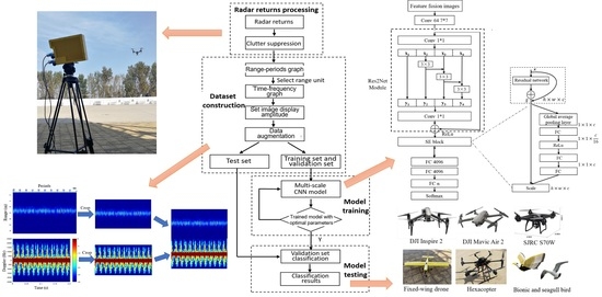
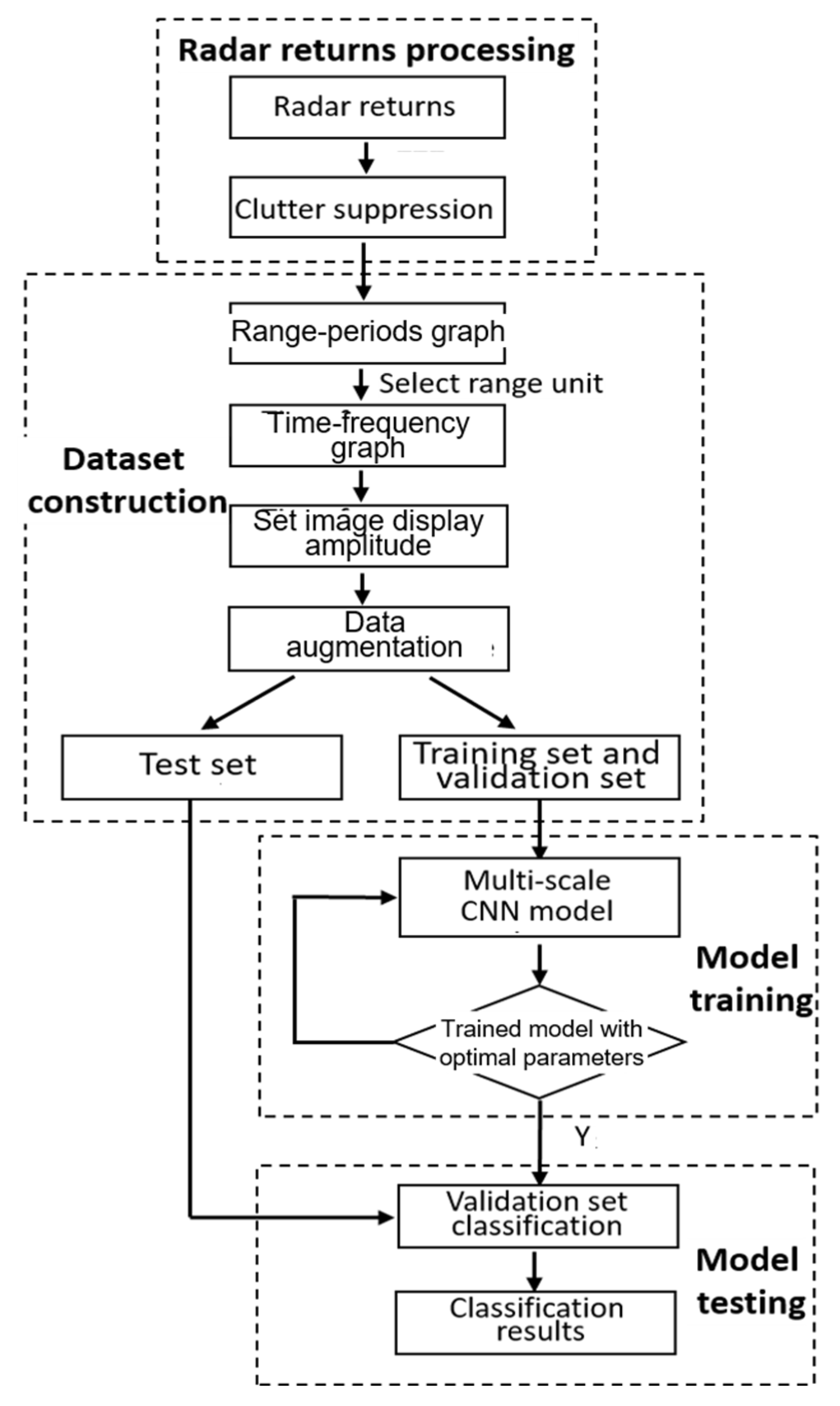
Figure 3 shows the data acquisition and signal processing flowchart of K-band FMCW radar. The processing results obtained after data acquisition are shown in Figure 4, which are a one-dimensional range profile (after demodulation), range-period graph, range-period graph after stationary clutter suppression and T-F graph of the target’s range unit. Figure 4c,d can accurately reflect the location and micro-motion information of the target, which are also the basis of the following m-D dataset.
The measurement principle of FMCW (triangular wave) radar for detecting relative moving target is shown in Figure 5. ft is the transmitted modulated signal, fr is the received reflected signal, B is the signal modulation bandwidth, f0 is the initial frequency of the signal, fd is the Doppler shift, T is the modulation period of the signal, and τ is the time delay. For FMCW radar (triangular wave modulation mode), the range information and speed information between the radar and the target can be measured by the difference frequency signal Δ f a and Δ f b of the triangular wave for two consecutive cycles [23].
Then, the received signal after demodulation can be written as
S M   ×   N = { s ( i , j ) | i = 1 , 2 , , M ;   j = 1 , 2 , , N }
where M represents the number of range unit and N is the samplings during the modulation periods.
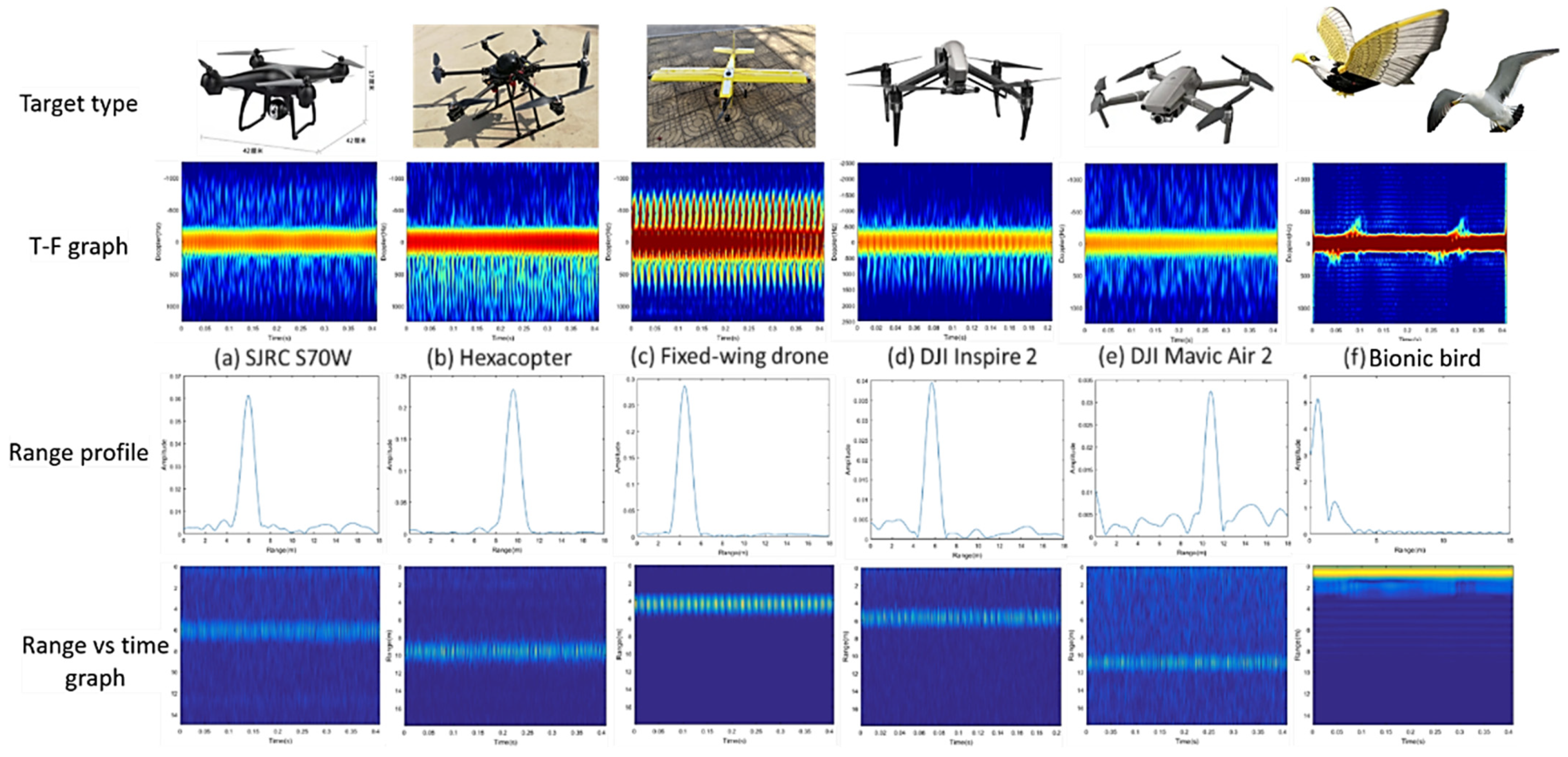
The feature selection of target’s signal includes high-resolution range-period and m-D features. The former can reflect the property of radar cross section (RCS) and the range walk information. The latter can obtain the characteristic of the vibration and rotation of the target and its components. At present, moving target classification usually uses T-F information, while the characteristics of range profile and range walk are ignored. Moreover, it cannot bring in additional effective features using traditional image augmentation methods, such as image rotation, cropping, blurring, and adding noise. It only generates similar images with the original images, and as the increment of expanded dataset, the similar data will also lead to network overfitting and poor generalization. In this paper we proposed three methods for effective data enhancement.
In Method 1, the display of range unit in the range-time/period graph is selected and focused on the target location to obtain the most obvious radar m-D characteristics of flying birds and rotary drones.
In Method 2, the amplitude scope displayed in T-F graph is adjusted to enhance the m-D features, and then the detail features of m-D are more obvious in the spectrum.
In Method 3, the above two methods can be combined together, i.e., adjusting different range units and setting different amplitude scopes. The advantage of the proposed data augmentation is that more different data can be fed into the classification model, and more feature information can be learned from the m-D signals.
The detailed data augmentation is described as follows:
Step 1: The target’s range unit is selected from the range-time/period graph, and T-F transform is performed on the time dimension data of a certain range unit to obtain the two-dimensional T-F graph, i.e., STFT s ( t , ω ) .
STFT s ( t , ω ) = + S M × N ( u ) g ( u t ) e j ω ( u t ) d u
where S M × N ( u ) is the demodulated signal or the signal after MTI processing, g ( u t ) is a movable window function and the variable parameter is the window length of the STFT.
Step 2: The amplitude is firstly normalized to [0, 1]. For the obtained range-time/period graph and T-F graph, the dataset is expanded by changing the display scope (spectrum amplitude). By controlling the color range display of the m-D feature in the T-F graph and the range-time/period graph, the m-D feature of the target and the range walk information can be enhanced or weakened.
The data in the range-time/period graph and T-F graph can be regarded as an array C, which is displayed by imagesc ( C ,   clims ) . The color range (spectrum amplitude) is specified as a two-element vector of the form clims = [ cmin   cmax ] . According to the characteristic display of the graph, different color ranges can be set appropriately to obtain different number of datasets. Take the drone as an example: set the color display for the range-periods graph to [A, 1] and specify the value of A as 0.01, 0.0001, and 0.00001. Then, the range-periods graph drawn in dB is shown in Figure 6. The drone target is located at 1 m, and different amplitude modulation features are given. Set the color display range for the T-F graph to [B, 1] and specify the values of B as 0.01, 0.0001 and 0.00001, respectively. The dataset augmentation of the T-F graph drawn in dB is shown in Figure 7.
Step 3: The dataset is performed by cropping, feature fusion and label calibration.
Based on the original range-period graph and T-F graph, select an area containing the target micro-motion feature for cropping, and the cropped image contains the target micro-movement feature in the uniform size. Feature fusion is to merge the range-period graph and T-F graph of the cropped image, which contains the target’s micro-motion features. The width of the range-period graph and T-F graph are consistent with the categories of different micro-motions. Then, label calibration of the dataset after feature fusion is performed for unified size. The feature fusion processing is shown in Figure 8.

3.2. Datasets Construction

We selected civilian-grade large, medium and small drones as typical rotary drones, i.e., the SJRC S70 W, DJI Mavic Air 2, DJI Inspire 2, six-rotor drone (hexacopter) and single-propeller fixed-wing drone, and flying bird targets (bionic and seagull birds). Figure 9 and Table 2 show the photos and main parameters of the different targets.
The M-D dataset of different types of drones and flying birds is shown in Table 3 and Figure 10. The construction of the micro-motion dataset mainly includes two parts: data preprocessing and data augmentation. The preprocessing mainly performs stationary clutter suppression via MTI (sometimes MTI is not a necessary step). The dataset can be expanded by setting the energy display amplitude of different m-D features. Cut the effective information of the range-periods and m-D spectrogram separately, and then combine the time-range information and the time-Doppler information to realize enhancement of the micro-motion features. In order to achieve the training of the CNN model, it is necessary to modify the dataset, remove the scale and colorbar of the horizontal and vertical axes of the input images, and normalize their sizes.

3.2.1. M-D Analysis of Small Drones, i.e., Mavic Air 2 and Inspire 2

The experimental scene is shown in Figure 11. According to the measured m-D characteristic image of the rotor drone in Figure 12, it can be seen that the echo intensity mainly located at zero frequency and its surroundings is very strong, which reflects the main body motion and micro-motion. The T-F graph of the “Inspire 2”, i.e., Figure 12b, has clearer m-D features than that of the “Mavic Air 2” in Figure 12a.
Figure 13 shows the m-D characteristics of Mavic Air 2 at different distances, i.e., 3 m, 6 m, 9 m and 12 m. As the distance increases, the m-D characteristics caused by the rotor are gradually weakened and its maximum Doppler amplitude is decreased, which is due to the weakening of the rotor echo. Although the m-D signal has been weakened, the reflection characteristics of the root of the rotor are still obvious, which is shown as a small modulation characteristic near the frequency of the main body’s motion.

3.2.2. M-D Analysis of Flying Birds

Due to the maneuverability of the real flying bird, the amount of bird radar data is limited. This paper collects two types of bird data: one is the indoor experiment using a bionic bird that highly simulates the flapping flight of real bird, and the other is the outdoor experiment for a real seagull bird. The subjects of the indoor experiment are a single bird and two birds with flapping wings, which is shown in Figure 14. The m-D characteristics are shown in Figure 15a,b. It can be found that the m-D effect produced by the flapping wings of a bird can be effectively observed by the experimental radar. According to the waveform frequency and maximum Doppler of the m-D characteristic in the figure, we can further estimate the wingspan length and flapping frequency of the bird. When simulating the side-by-side flapping movement of two birds, the micro-motion characteristics in the T-F domain may be overlapped.
The outdoor experiment for real bird micro-motion signal acquisition is carried out. The observation distance is 3 m and other parameters remain unchanged. The obtained m-D characteristics of real bird flight are shown in Figure 16. According to the T-F graph, the m-D effect of the flapping wings can be observed as well and there are both similarities and differences of m-D features between the real birds and bionic bird. The similarity lies in the obvious periodic characteristics of the micro-motions, with longer interval and stronger amplitude, which are also distinctive features from drone targets. The difference is that m-D signal of the real bird is relatively weak due to the far distance, and there are some subtle fluctuations. However, the overall micro-motion characteristics different from the rotary-wing drones are obvious, and therefore the indoor and outdoor bird data are combined together as the overall dataset for further training and testing.

3.2.3. M-D Analysis of Fixed-Wing Drone

Figure 17 shows the micro-motion characteristics of the fixed-wing drone. In order to better analyze the influence of different observation angles on the m-D, results of three observation angles, i.e., side view, front view, and up view, are provided respectively. The following conclusions can be drawn by comparison.
  • When the radar is looking ahead, the echo is the strongest (Figure 17b), with very obvious Doppler periodic modulation characteristics. Due to the low rotation speed, the micro-motion period is significantly longer than that of the rotary-wing drone.
  • Compared Figure 17b,c, i.e., different observation elevation angles, it can be seen that there is an optimal observation angle for radar detection of the target. When the observation angle changes, the m-D characteristics will be weakened to a large extent and the micro-motion information would be partially missing. In addition, when the radar is observing the target vertically (side view Figure 17a), the radial velocity of the blade towards the radar is the biggest, which results in the maximum Doppler effect compared to the other two angles.
  • Due to the large size of the fixed-wing drone and the blades, the main body echo and the m-D characteristics of the blades are significantly stronger than those of the rotary-wing drone and the flying bird.
  • As the blade speed increases, the micro-motion modulation period becomes shorter and part of the micro-motion feature is missing.

3.2.4. M-D Analysis of Hexacopter Drone

Figure 18 shows the m-D characteristics of the six-axis rotor drone, i.e., hexacopter, at two distances. Figure 18a,c shows a range versus modulation periods graph. It can be clearly seen that there are obvious echoes around 11.5 m and 8.5 m, respectively, and the radar range resolution is 7.5 cm (bandwidth is 2 GHz). Under high-resolution conditions, due to the rotation of the rotors, the drone’s echo occupies multiple range units and exhibits obvious periodic changes. Due to the different lengths and sizes of the rotors, various extended range units and modulation periods characteristics can be reflected in the range-periods graph, which verifies the usefulness of the range-period information. Due to the multiple rotors and the fast rotation speed, the micro-motion components in the T-F graph (Figure 18b,d) overlap with each other. The positive-frequency of micro-motion characteristics caused by the rotation of the rotor, i.e., towards the radar, are more obvious than the other part. Large rotors would result in obvious periodic modulation characteristics near the main body, which is also helpful for subsequent classification.

3.3. The Modified Multi-Scale CNN Model

This paper proposes a target m-D feature classification method based on the modified multi-scale CNN [25], which uses multi-scale splitting of the hybrid connection structure. The output of the multi-scale module contains a combination of different receptive field sizes, which is conducive to extracting the global feature information and the local information of the target. Firstly, a single-layer convolution kernel with a 7 × 7 convolutional layer is used to extract features from the input image, and then a multi-scale network characterization module is employed. The 1 × 1 convolution kernel is used to adjust the number of input channels, so that the next multi-scale module can perform in-depth feature extraction. The structure of the multi-scale CNN model is shown in Figure 19, which is based on the residual network module (Res2 Net). The filter bank with a convolution kernel size of 3 × 3 is used to replace the 1 × 1 convolutional feature map of n channels. The feature map after 1 × 1 convolution of two channels is divided into s feature map subsets, and each feature map subset contains n/s number of channels. Except for the first feature map subset that is directly passed down, the rest of the feature map subsets are followed by a convolutional layer with a convolution kernel size of 3 × 3, and the convolution operation is performed.
The second feature map subset is convoluted, and a new feature subset is formed and passed down in two lines. One line is passed down directly; and the other line is combined with the third feature map subset using a hierarchical arrangement connection method and sent to the convolution to form a new feature map subset. Then, the new feature map subset is divided into two lines; one is directly passed down, and the other line is still connected with the fourth feature map subset using a hierarchical progressive arrangement and sent to the convolutional layer to obtain other new feature map subsets. Repeat the above operations until all feature map subsets have been processed. Each feature map subset is combined with another feature map subset after passing through the convolutional layer. This operation will increase the equivalent receptive field of each convolutional layer gradually, so as to complete the extraction of information at different scales.
Use Ki() to represent the 3 × 3 output of the convolution kernel, and xi represents the divided feature map subsets, where i { 1 , 2 , , s } and s represents the number of feature map subsets divided by the feature map. The above process can be expressed as follows
y 1 = x 1 y 2 = K 2 ( x 2 ) y 3 = K 3 ( x 3 + y 2 ) = K 3 [ x 3 + K 2 ( x 2 ) ] y 4 = K 4 ( x 4 + y 3 ) = K 4 ( x 4 + K 3 [ x 3 + K 2 ( x 2 ) ] )
Then the output yi can be expressed as
y i = { x i K i ( x i ) K i ( x i + y i 1 ) i = 1 i = 2 2 < i s
Based on the above network structure, the output of the multi-scale module includes a combination of different receptive field sizes via the split hybrid connection structure, which is conducive to extracting global and local information. Specifically, the feature map after the convolution operation with the convolution kernel size of 1 × 1 is divided into four feature map subsets; after the multi-scale structure hybrid connection, the processed feature map subsets are combined by a splicing method, i.e., y1 + y2 + y3 + y4. A convolutional layer with convolution kernel size 1 × 1 is used on the spliced feature map subsets to realize the information fusion of the divided four feature map subsets. Then, the multi-scale residual module is combined with the identity mapping y = x.
The squeeze excitation (SE) module is added after the multi-scale residual module, and then the modified multi-scale neural network residual module is completed. The structure of the SE module is given in the right of 0. For a feature map with a shape of (h, w, c), i.e., (height, width, channel), the SE module first performs a compression operation, and the feature map is globally averaged in the spatial dimension to obtain a feature vector representing global information. Convert the output of the multi-scale residual module h   ×   w   ×   c into the output of 1   ×   1   ×   c . The second is the incentive operation, which is shown as follows.
S = F ex ( z , W ) = σ [ g ( z , W ) ] = σ [ W 2 × δ ( W 1   ×   z ) ]
where δ ( W 1   ×   z ) represents the first fully connected operation (FC), the first layer weight parameter is W1 whose dimension is c   ×   c / r , r is called the scaling factor.
Here, let r = 16, its function is to reduce the number of channels with less calculations, and z is the result of the previous squeeze operation with the dimension 1 × c. g(z, W) represents the output result after the first fully connected operation. After the first fully connected layer, the dimension becomes 1   ×   1   ×   c / 16 , and then a ReLu layer activation function is added to increase the nonlinearity of the network, while the output dimension remains unchanged. Then, it is multiplied by W2, i.e., weight of the second fully connected layer. The output dimension becomes 1   ×   1   ×   c and the output of the SE module is calculated through the activation function Sigmoid.
Finally, the re-weighting operation is performed, and the feature weights S are multiplied to the input feature map channel by channel to complete the feature re-calibration operation. This learning method can automatically obtain the importance of each feature channel, increase the useful features accordingly and suppress the features useless for the current task. The multi-scale residual module and the SE module are combined together and with 18 such modules the modified multi-scale network is formed. The combination of the multi-scale residual module and the SE module can learn different receptive field combinations and retain useful features, and suppress invalid feature information, which greatly reduces the parameter calculation burden. Finally, we add a three-layer fully connected layer. It is used to map the effective features learned by the multi-scale model to the label space of the samples; moreover, the depth of the network model is increased so that it can learn refined features. Compared with the global average pooling, the fully connected layer can achieve faster convergence speed and higher recognition accuracy.
By setting the parameter solving algorithm Adam, the nonlinear activation function ReLU, the initial learning rate 0.0001, the training round (Epoch) 100 and other parameters, the dataset is trained. After training for one round, a verification is performed on the verification set until the correct recognition rate meets the requirements, and the network model parameters are saved to obtain the suitable network model. The final test is to input the test data not involved in training and verification into the trained network model to verify the effectiveness and generalization ability of the multi-scale CNN model. By calculating the ratio of the number of samples correctly classified in the test dataset to the total number of samples in the entire test set, the classification accuracy is obtained.

3.4. Algorithm Flowchart

The detailed flowchart of the classification method for flying birds and rotary-wing drones based on the data augmentation and the multi-scale CNN is shown in Figure 20, which is consisted of four parts, radar echo processing, m-D dataset construction, CNN model training and model testing.

4. Experimental Results

All models are implemented on a PC equipped with 16 G memory, a 2.5 GHZ Intel(R) Core (TM) i5-8400 CPU and an NVIDIA GeForce GTX1050Ti GPU. In the experiment, we use the Adam algorithm as an optimizer, ReLu as the activation function and the cross entropy as cost function. The initial learning rate is set to 0.0001 and the number of iterations is 100. In addition, to prevent the overfitting problem, dropout is applied to improve model generalization ability. The size of the extracted spectrogram was 560 × 420 and normalized to 100 × 100 for data training in order to increase the computational speed.
Using the proposed method and the other popular CNNs, e.g., Alexnet and VGG16, the classification performance for five types of rotary-wing drones and flying bird is given by the confusion matrix under the conditions of relative short range (SNR > 0 dB) and relative long range (SNR < 0 dB). According to the analysis of Section 5.4, the detection probability of SNR = 0 dB is about 86.3% (normal value), therefore we choose 12 m as the boundary and when the range is farer than 12 m, it is called relative long range and vice versa. K-fold cross-validation method is employed in order to obtain a reliable and stable model [30] (K = 5 in this paper). For shorter range, Table 4, Table 5 and Table 6 show the confusion matrix of Alexnet, VGG16 and the proposed method for six targets, and the number of test samples for each type of target is 40. The true class is along the top. Target A judged as other types are represented in gray, i.e., there is no mutual judgment error; pink is the samples judged correctly; green color represents the cases of wrong classification, and dark green means more than one mistake.
It can be seen from Table 4 and Table 5 that it is difficult to distinguish the Mavic Air 2, SJRC S70 W and Hexacopter, and there are many wrong classification cases. Figure 21b–d shows the range-periods graph and T-F graph, which indicates that the three types of targets all have the micro-motion characteristics of the rotor. Because of the fast speed, the T-F graph is densely distributed with short period. However, there are also subtle differences. For example, the Hexacopter has a wide range of m-D spectrum and obvious micro-motion peaks, while the micro-motion spectrum of the Mavic Air 2 is concentrated around −200 Hz~200 Hz, due to its small rotor size. If better classification ability is needed, the network is required to be able to learn both of large-scale periodic modulation features and small-scale micro-motion features. Compared with Alexnet, the classification accuracy of the CNN based on VGG16 is higher, i.e., from 89.6% to 94.6%, but for small drones, there are still classification errors. Fixed-wing drones have a small number of rotors and exhibit obvious echo modulation characteristics. The Hexacopter drone has many rotors with larger size, and therefore it occupies more range units in the time domain (the white box in Figure 21b), which are also effective features different from small drones. Then, the modified multi-scale CNN is used to split the hybrid connection structure at multiple scales, so that the output of the multi-scale module contains a combination of different receptive field sizes, which is conducive to extracting the global and local information of the target features. The classification accuracy probability is increased to 99.2%.
For longer ranges, the confusion matrices are shown in Table 7, Table 8 and Table 9. As the target echo gets weaker, the m-D characteristics also become inconspicuous. Therefore, for Alexnet, it is difficult to distinguish the three smaller sizes targets, i.e., the Mavic Air 2, SJRC S70 W and Inspire 2, as shown in Figure 22b,c. At the same time, it is easy to judge the Hexacopter as Mavic Air 2, because the spectrum broadening feature of the Hexacopter is not obvious, as shown in Figure 22a. The proposed method can learn the weak and broadened spectrum characteristics, thereby improving the classification probability to 97.5% compared with the other two models, at 88.3% and 92.9%. Based on the above analysis, the proposed method has a good classification ability for different types of rotary-wing drones, and can distinguish flying bird targets as well.

5. Discussion

5.1. The Influence of Amplitude Display on Classification

The spectrum amplitude display is set from clim (10−2) to clim (10−6), and it is found that the m-D spectrum becomes more and more significant. When the amplitude of the spectrum was set to clim (10−6), the Doppler energy was found to be more divergent and even some glitches appeared. On the contrary, when the amplitude of the spectrum is at clim (10−2), the m-D feature disappears or is weakened. In addition, we construct a dataset with different clim values to study the effect of spectrum amplitude display on micro-motion classification. The comparison results of different clim are shown in Table 10. One fold corresponds to the accuracy of each training. It can be observed that the classification accuracy of target classification is getting higher and higher as the number of dataset increases. It is noted that the expansion of the dataset plays a key role in improving the accuracy of the target classification. One phenomenon we find is that the recognition accuracy of clim (10−4) in the same dataset is higher than that without clim (10−4), such as the recognition accuracy of C1 and C3 being higher than that of C2. The result shows that the spectrum with clim (10−4) has the best m-D characteristics for m-D classification.

5.2. Classification Performance Using Feature Fusion Strategy

In order to further compare the impact of the feature fusion method proposed in Section 3.1 on the classification performance, the results of the single range-period graph dataset, the T-F graph dataset and the feature fusion dataset are compared, as shown in Table 11. Each dataset is trained three times and averaged as the final classification accuracy. Experiments show that the classification accuracy using feature fusion strategy is 31% and 6% higher than the classification accuracy of the single range-period graph and T-F graph datasets, respectively.

5.3. Classification Performance via Different Network Models

The superiority of the modified multi-scale network model structure is verified and the two typical ResNet18 and Res2Net18 network models are compared under the same conditions (the network layer depth is the same as 18 layers and the SE module is added). The result is shown in Figure 23. The classification accuracy of Resnet, Res2Net and the modified multi-scale network model on the validation set are as follows: 93.9%, 95.06% and 96.9%, respectively, indicating that the modified model has better classification accuracy.

5.4. Detection Probability for Different Ranges and SNRs

Since the radar used in this paper is a FMCW radar, the detection range for such low-observable drones or birds is limited. In order to prove the universality of the proposed method and further generalize the conclusions, the detection performance with different signal-to-noise ratios (SNRs) of the returned signal is employed as a parameter to show how far to detection the target instead of the range parameter. The SNR is defined as the average power ratio of target’s range unit to the background unit in the range-period data. Table 12 gives the detection probability of Mavic Air 2 under different SNRs. Its maximum detection range is about 100 m according to the radar range equation. The data were recorded for different ranges and we give the relation between the target’s location and the SNR. The detection process is carried out in the two dimension data, i.e., range-period, with the CA-CFAR, and the false alarm rate is 10−2. It should be noted that the relation is only for Mavic Air 2 using the FMCW radar in the paper and we assume the target can be detected for the following analysis of classification.
It should be noted that the proposed algorithm is based on the correct detection of the target (exceeding the threshold), and the obvious m-D characteristics. Therefore, the result of clutter suppression and m-D signal enhancement would affect the classification results. Although due to the low power of the FMCW radar and the small RCS of the drone, the signal is weak and the detection range is relatively short, the conclusion can be applied to other radars according to the SNR relations (Table 12).

6. Conclusions

A feature extraction and classification method of flying birds and rotor drones is proposed based on data augmentation and a modified multi-scale CNN. The m-D signal models of the rotary drone and flying birds are established. Multi-features, i.e., the range profile, range-time/periods and m-D features (T-F graph), are employed and a data augmentation method is proposed by setting the color display amplitude of the T-F spectrum in order to increase the effective dataset and enhance m-D features. Using a K-band FMCW radar, micro-motion signal measurement experiments were carried out for five different sizes of rotary drones and one bionic bird, i.e., the SJRC S70 W, DJI Mavic Air 2, DJI Inspire 2, hexacopter and single-propeller fixed-wing drone. Different observation conditions on the impact of m-D characteristics, e.g., angle, distance, rotating speed, etc., were analyzed and compared. The multi-scale CNN model was modified for better learning and distinguishing of different micro-motion features, i.e., global and local information of m-D features. The experimental results for different scenes (indoor, outdoor, high SNR and low SNR) show that the proposed method has better classification accuracy of the five types of drones and flying birds compared with popular methods, e.g., AlexNet and VGG16. In future research, in order to better analyze the target classification performance for long distance and clutter background, the coherent pulse-Doppler radar will be used and the target’s characteristics, e.g., m-D, will be investigated. Further, the CNN may be more intelligent with the intelligent systems, which enables truly intelligent processing and recognition [31].

7. Patents

The methods described in this article have applied for a Chinese invention patent: “A dataset expansion method and system for radar micro-motion target recognition. Patent number: 2020121101990640”; “A radar target micro-motion feature extraction and intelligent classification method and system. Patent number: 202110818621.0”.

Author Contributions

Conceptualization, X.C.; methodology, X.C.; software, J.L.; validation, J.L. and H.Z.; formal analysis, Z.H.; investigation, J.G. and J.S.; resources, J.G.; data curation, X.C. and J.S.; writing—original draft preparation, X.C. and J.L.; writing—review and editing, X.C.; visualization, Z.H.; supervision, J.G.; project administration, X.C.; funding acquisition, X.C. All authors have read and agreed to the published version of the manuscript.

Funding

This research was supported by Shandong Provincial Natural Science Foundation, grant number ZR2021YQ43, National Natural Science Foundation of China, grant number U1933135, 61931021, partly funded by the Major Science and Technology Project of Shandong Province, grant number 2019JZZY010415.

Institutional Review Board Statement

Not applicable.

Informed Consent Statement

Not applicable.

Data Availability Statement

Not applicable.

Acknowledgments

The authors would like to thank Libao Wang for the help of the FMCW radar.

Conflicts of Interest

The authors declare no conflict of interest.

References

  1. Chen, X.; Chen, W.; Rao, Y.; Huang, Y.; Guan, J.; Dong, Y. Progress and prospects of radar target detection and recognition technology for flying birds and unmanned aerial vehicles. J. Radars 2020, 9, 803–827. [Google Scholar] [CrossRef]
  2. Gong, J.; Yan, J.; Li, D.; Chen, R. Using Radar Signatures to Classify Bird Flight Modes Between Flapping and Gliding. IEEE Geosci. Remote Sens. Lett. 2019, 17, 1518–1522. [Google Scholar] [CrossRef]
  3. Flock, W.L.; Green, J.L. The detection and identification of birds in flight, using coherent and noncoherent radars. Proc. IEEE 1974, 62, 745–753. [Google Scholar] [CrossRef]
  4. Chen, X.; Guan, J.; Chen, W.; Zhang, L.; Yu, X. Sparse long-time coherent integration–based detection method for radar low-observable maneuvering target. IET Radar Sonar Navig. 2020, 14, 538–546. [Google Scholar] [CrossRef]
  5. Taha, B.; Shoufan, A. Machine Learning-Based Drone Detection and Classification: State-of-the-Art in Research. IEEE Access 2019, 7, 138669–138682. [Google Scholar] [CrossRef]
  6. Park, J.; Jung, D.-H.; Bae, K.-B.; Park, S.-O. Range-Doppler Map Improvement in FMCW Radar for Small Moving Drone Detection Using the Stationary Point Concentration Technique. IEEE Trans. Microw. Theory Tech. 2020, 68, 1858–1871. [Google Scholar] [CrossRef]
  7. Chen, V.C.; Li, F.; Ho, S.; Wechsler, H. Micro-Doppler effect in radar: Phenomenon, model, and simulation study. IEEE Trans. Aerosp. Electron. Syst. 2006, 42, 2–21. [Google Scholar] [CrossRef]
  8. Li, G.; Zhang, R.; Ritchie, M.; Griffiths, H. Sparsity-Driven Micro-Doppler Feature Extraction for Dynamic Hand Gesture Recognition. IEEE Trans. Aerosp. Electron. Syst. 2017, 54, 655–665. [Google Scholar] [CrossRef]
  9. Du, L.; Li, L.; Wang, B.; Xiao, J. Micro-Doppler Feature Extraction Based on Time-Frequency Spectrogram for Ground Moving Targets Classification with Low-Resolution Radar. IEEE Sens. J. 2016, 16, 3756–3763. [Google Scholar] [CrossRef]
  10. Li, T.; Wen, B.; Tian, Y.; Li, Z.; Wang, S. Numerical Simulation and Experimental Analysis of Small Drone Rotor Blade Polarimetry Based on RCS and Micro-Doppler Signature. IEEE Antennas Wirel. Propag. Lett. 2019, 18, 187–191. [Google Scholar] [CrossRef]
  11. Kim, B.K.; Kang, H.-S.; Park, S.-O. Experimental Analysis of Small Drone Polarimetry Based on Micro-Doppler Signature. IEEE Geosci. Remote Sens. Lett. 2017, 14, 1670–1674. [Google Scholar] [CrossRef]
  12. Gong, J.; Yan, J.; Li, D.; Chen, R.; Tian, F.; Yan, Z. Theoretical and Experimental Analysis of Radar Micro-Doppler Signature Modulated by Rotating Blades of Drones. IEEE Antennas Wirel. Propag. Lett. 2020, 19, 1659–1663. [Google Scholar] [CrossRef]
  13. Singh, A.K.; Kim, Y.-H. Automatic Measurement of Blade Length and Rotation Rate of Drone Using W-Band Micro-Doppler Radar. IEEE Sens. J. 2017, 18, 1895–1902. [Google Scholar] [CrossRef]
  14. Oh, B.-S.; Guo, X.; Wan, F.; Toh, K.-A.; Lin, Z. Micro-Doppler Mini-UAV Classification Using Empirical-Mode Decomposition Features. IEEE Geosci. Remote Sens. Lett. 2017, 15, 227–231. [Google Scholar] [CrossRef]
  15. Zhu, L.; Zhang, S.; Ma, Q.; Zhao, H.; Chen, S.; Wei, D. Classification of UAV-to-Ground Targets Based on Enhanced Micro-Doppler Features Extracted via PCA and Compressed Sensing. IEEE Sens. J. 2020, 20, 14360–14368. [Google Scholar] [CrossRef]
  16. Kim, B.K.; Kang, H.-S.; Park, S.-O. Drone Classification Using Convolutional Neural Networks with Merged Doppler Images. IEEE Geosci. Remote Sens. Lett. 2016, 14, 38–42. [Google Scholar] [CrossRef]
  17. Wang, C.; Tian, J.; Cao, J.; Wang, X. Deep Learning-Based UAV Detection in Pulse-Doppler Radar. IEEE Trans. Geosci. Remote Sens. 2021, 60, 1–12. [Google Scholar] [CrossRef]
  18. Zhu, J.; Chen, H.; Ye, W. A Hybrid CNN–LSTM Network for the Classification of Human Activities Based on Micro-Doppler Radar. IEEE Access 2020, 8, 24713–24720. [Google Scholar] [CrossRef]
  19. Ai, J.; Tian, R.; Luo, Q.; Jin, J.; Tang, B. Multi-Scale Rotation-Invariant Haar-Like Feature Integrated CNN-Based Ship Detection Algorithm of Multiple-Target Environment in SAR Imagery. IEEE Trans. Geosci. Remote Sens. 2019, 57, 10070–10087. [Google Scholar] [CrossRef]
  20. Chen, X.; Su, N.; Huang, Y.; Guan, J. False-Alarm-Controllable Radar Detection for Marine Target Based on Multi Features Fusion via CNNs. IEEE Sens. J. 2021, 21, 9099–9111. [Google Scholar] [CrossRef]
  21. Chen, X.; Mu, X.; Guan, J.; Liu, N.; Zhou, W. Marine target detection based on Marine-Faster R-CNN for navigation radar PPI images. Front. Inf. Technol. Electron. Eng. 2022; in press. [Google Scholar]
  22. Chen, X.; Guan, J.; Mu, X.; Wang, Z.; Liu, N.; Wang, G. Multi-Dimensional Automatic Detection of Scanning Radar Images of Marine Targets Based on Radar PPInet. Remote Sens. 2021, 13, 3856. [Google Scholar] [CrossRef]
  23. Rai, P.K.; Idsøe, H.; Yakkati, R.R.; Kumar, A.; Khan, M.Z.A.; Yalavarthy, P.K.; Cenkeramaddi, L.R. Localization and activity classification of unmanned aerial vehicle using mmwave FMCW radars. IEEE Sens. J. 2021, 21, 16043–16053. [Google Scholar] [CrossRef]
  24. Shin, D.-H.; Jung, D.-H.; Kim, D.-C.; Ham, J.-W.; Park, S.-O. A Distributed FMCW Radar System Based on Fiber-Optic Links for Small Drone Detection. IEEE Trans. Instrum. Meas. 2017, 66, 340–347. [Google Scholar] [CrossRef]
  25. Gao, S.-H.; Cheng, M.-M.; Zhao, K.; Zhang, X.-Y.; Yang, M.-H.; Torr, P. Res2Net: A new multi-scale backbone architecture. IEEE Trans. Pattern Anal. Mach. Intell. 2021, 43, 652–662. [Google Scholar] [CrossRef] [PubMed] [Green Version]
  26. Sun, L.; Liu, Z.; Sun, X.; Liu, L.; Lan, R.; Luo, X. Lightweight Image Super-Resolution via Weighted Multi-Scale Residual Network. IEEE/CAA J. Autom. Sin. 2021, 8, 1271–1280. [Google Scholar] [CrossRef]
  27. Krizhevsky, A.; Sutskever, I.; Hinton, G. ImageNet classification with deep convolutional neural networks. In Proceedings of the 25th International Conference on Neural Information Processing Systems, Lake Tahoe, CA, USA, 1 December 2012; pp. 1097–1105. [Google Scholar]
  28. Simonyan, K.; Zisserman, A. Very deep convolutional networks for large-scale image recognition. arXiv 2014, arXiv:1409.1556. [Google Scholar]
  29. Ritchie, M.; Fioranelli, F.; Griffiths, H.; Torvik, B. Monostatic and bistatic radar measurements of birds and micro-drone. In Proceedings of the 2016 IEEE Radar Conference (RadarConf), Philadelphia, PA, USA, 2–6 May 2016; pp. 1–5. [Google Scholar] [CrossRef] [Green Version]
  30. Moreno-Torres, J.G.; Saez, J.A.; Herrera, F. Study on the Impact of Partition-Induced Dataset Shift on k-Fold Cross-Validation. IEEE Trans. Neural Netw. Learn. Syst. 2012, 23, 1304–1312. [Google Scholar] [CrossRef]
  31. Iantovics, L.B.; Iakovidis, D.K.; Nechita, E. II-Learn—A Novel Metric for Measuring the Intelligence Increase and Evolution of Artificial Learning Systems. Int. J. Comput. Intell. Syst. 2019, 12, 1323. [Google Scholar] [CrossRef] [Green Version]
Figure 1. Flying bird flapping motion model. (a) The front view; (b) The top view.
Remotesensing 14 01107 g001
Figure 2. The geometric diagram of radar and quadrotor drone.
Remotesensing 14 01107 g002
Figure 3. Description K-band FMCW radar. (a) Radar and computer terminal connection diagram; (b) System operation and signal processing flowchart.
Remotesensing 14 01107 g003
Figure 4. Processing results obtained after data collection. (a) Range profile (after demodulation); (b) Range-period graph after stationary clutter suppression; (c) Range-period graph; (d) T-F graph of the target’s range unit.
Remotesensing 14 01107 g004
Figure 5. The schematic diagram of FMCW radar measurement.
Remotesensing 14 01107 g005
Figure 6. Dataset augmentation of range-period graph. (a) [−20, 0] dB; (b) [−40, 0] dB; (c) [−50, 0] dB.
Remotesensing 14 01107 g006
Figure 7. The dataset augmentation of the T-F graph. (a) [−20, 0] dB; (b) [−40, 0] dB; (c) [−50, 0] dB.
Remotesensing 14 01107 g007
Figure 8. Feature fusion of the datasets.
Remotesensing 14 01107 g008
Figure 9. Pictures of different categories of drones and flying bird.
Remotesensing 14 01107 g009
Figure 10. M-D datasets of different types of drones and flying bird.
Remotesensing 14 01107 g010
Figure 11. Outdoor experiment of small drone data collection using FMCW Radar. (a) DJI Mavic Air 2; (b) DJI Inspire 2.
Remotesensing 14 01107 g011
Figure 12. M-D of small drones for outdoor experiment. (a) DJI Mavic Air 2; (b) DJI Inspire 2.
Remotesensing 14 01107 g012
Figure 13. The m-D characteristics of Mavic Air2 at different distances. (a) 3 m; (b) 6 m; (c) 9 m; (d) 12 m.
Remotesensing 14 01107 g013aRemotesensing 14 01107 g013b
Figure 14. The indoor experimental scene of bionic flying birds. (a) Single bird; (b) Two birds.
Remotesensing 14 01107 g014
Figure 15. The m-D characteristics of bionic flying birds (indoor experiment). (a) Single bird; (b) Two bionic birds.
Remotesensing 14 01107 g015
Figure 16. The m-D characteristics of real flying birds (outdoor experiment). (a) Bird A; (b) Bird B.
Remotesensing 14 01107 g016
Figure 17. M-D characteristics of fixed wing drone for different observation views. From the side view, range 2.3 m: (a1) Low speed; (a2) High speed; (a3) Scene photo. From the front view range 4 m: (b1) Low speed; (b2) High speed; (b3) Scene photo. From the up view, range 8 m: (c1) Low speed; (c2) High speed; (c3) Scene photo.
Remotesensing 14 01107 g017
Figure 18. M-D characteristics of hexacopter drone. Data 1: (a) Range vs periods (after MTI); (b) T-F graph. Data 2: (c) Range vs. periods (after MTI); (d) T-F graph.
Remotesensing 14 01107 g018
Figure 19. The multi-scale CNN structure. The right picture is an enlarged view of the SE module.
Remotesensing 14 01107 g019
Figure 20. Micro-motion classification flowchart of flying bird and drone target.
Remotesensing 14 01107 g020
Figure 21. Range-periods and T-F graph for relative short range (4–8 m). (a) Fixed-wing; (b) Hexacopter; (c) SJRC S70 W; (d) Mavic Air 2.
Remotesensing 14 01107 g021
Figure 22. Range-periods and T-F graph for relative long range (11–13 m). (a) Hexacopter; (b) Inspire 2; (c) Mavic Air 2.
Remotesensing 14 01107 g022
Figure 23. Comparison of classification accuracy using different network models.
Remotesensing 14 01107 g023
Table 1. Main parameters of the K-band FMCW radar.
ParametersValue
Working frequency23.8 GHz
Modulation bandwidth10 MHz~2 GHz
Modulation period0.2 ms~40 ms
Transmitting power10 dBm
−3 db beamwidthAzimuth: 16 degree; Elevation: 12 degree
Table 2. Target parameters of different types of birds and drones.
TypesNameAbbreviationType *Number of RotorsLength of Rotor (cm)
1HexacopterHQ638
2DJI Inspire 2IQ438
3Fixed-wing droneFP230
4DJI Mavic Air 2MQ422
5SJRC S70 WSQ423
6Flying birdBB2 #22 #
* Type “Q” is for quadrocopter, “P” is for plane, “B” is for bird. # The target parameters of the bird are expressed as the number of wings and half the length of the bird’s wingspan.
Table 3. The composition of the micro-motion classification dataset (Each data lasts about 0.4 s).
DataTraining DataValidation DataTesting Data
Types
Mavic Air 272018040
Inspire 272018040
SJRC S70 W72018040
Hexacopter72018040
Fixed-wing72018040
Flying bird72018040
Total43201080240
Table 4. Confusion matrix of Alexnet for relative short range (average classification accuracy 89.6%).
MethodMavic Air 2SJRC S70 WInspire 2HexacopterFixed-WingFlying Bird
M3221100
S4321400
I1138000
H3503510
F0000380
B0000140
Table 5. Confusion matrix of VGG16 for relative short range (average classification accuracy 94.6%).
ClassMavic Air 2SJRC S70 WInspire 2HexacopterFixed-WingFlying Bird
M3510000
S2361200
I1039000
H2303810
F0000390
B0000040
Table 6. Confusion matrix of the proposed method for relative short range (average classification accuracy 99.2%).
ClassMavic Air 2SJRC S70 WInspire 2HexacopterFixed-WingFlying Bird
M3910000
S1390000
I0040000
H0004000
F0000400
B0000040
Table 7. Confusion matrix of Alexnet for relative long range (average classification accuracy 88.3%).
ClassMavic Air 2SJRC S70 WInspire 2HexacopterFixed-WingFlying Bird
M3231200
S4321000
I2236110
H2323702
F0000381
B0000137
Table 8. Confusion matrix of VGG16 for relative long range (average classification accuracy 92.9%).
ClassMavic Air 2SJRC S70 WInspire 2HexacopterFixed-WingFlying Bird
M3411200
S3370000
I2237200
H1023600
F0000401
B0000039
Table 9. Confusion matrix of the proposed method for relative long range (average classification accuracy 97.5%).
ClassMavic Air 2SJRC S70 WInspire 2HexacopterFixed-WingFlying Bird
M3810000
S1380000
I1139100
H0013900
F0000400
B0000040
Table 10. Classification accuracy results of the different clims.
MethodsDatasetFold 1Fold 2Fold 3Average
C1clim (10−3, 10−4)96.96%96.57%96.61%96.71%
C2clim (10−3, 10−5)95.42%95.39%95.40%95.40%
C3clim (10−4, 10−5)96.11%96.37%96.96%96.48%
C4clim (10−3, 10−4, 10−5)98.13%97.26%97.48%97.62%
C5clim (10−2, 10−3, 10−4, 10−5)98.61%98.28%98.48%98.46%
C6clim (10−2, 10−3, 10−4,10−5, 10−6)98.90%98.65%98.71%98.75%
Table 11. Classification accuracy results using feature fusion strategy.
Training Times123Average
Dataset
Range-period graph65.20%63.83%67.61%65.54%
T-F graph90.34%90.85%90.27%90.49%
Feature fusion97.01%96.9%96.93%96.94%
Table 12. Detection probability for different ranges (Mavic Air 2).
SNR = −6 dB
(About 50 m)
SNR = −3 dB
(About 20 m)
SNR = 0 dB
(About 12 m)
SNR = 2 dB
(About 8 m)
SNR = 5 dB
(About 6 m)
Detection Probability75.9%80.7%86.3%93.2%99.1%
Publisher’s Note: MDPI stays neutral with regard to jurisdictional claims in published maps and institutional affiliations.

