Space-Based Detection of Significant Water-Depth Increase Induced by Hurricane Irma in the Everglades Wetlands Using Sentinel-1 SAR Backscatter Observations

Abstract

Extreme rainfall, induced by severe weather events, such as hurricanes, impacts wetlands because rapid water-depth increases can lead to flora and fauna mortality. This study developed an innovative algorithm to detect significant water-depth increases (SWDI, defined as water-depth increases above a threshold) in wetlands, using Sentinel-1 SAR backscatter. We used Hurricane Irma as an example that made landfall in the south Florida Everglades wetlands in September 2017 and produced tremendous rainfall. The algorithm detects SWDI for during- and post-event SAR acquisition dates, using pre-event water-depth as a baseline. The algorithm calculates Normalized Difference Backscatter Index (NDBI), using pre-, during-, and post-event backscatter, at a 20-m SAR resolution, as an indicator of the likelihood of SWDI, and detects SWDI using all NDBI values in a 400-m resolution pixel. The algorithm successfully detected large SWDI areas for the during-event date and progressive expansion of non-SWDI areas (water-depth differences less than the threshold) for five post-event dates in the following two months. The algorithm achieved good performance in both ‘herbaceous dominant’ and ‘trees embedded within herbaceous matrix’ land covers, with an overall accuracy of 81%. This study provides a solution for accurate mapping of SWDI and can be used in global wetlands, vulnerable to extreme rainfall.

1. Introduction

Wetlands are productive ecosystems that provide various services, including habitats for many plant and animal species, water supply and purification, carbon sequestration, coastal protection, and outdoor recreation. Hydrology is the most important abiotic factor controlling wetland functions [1]. For many wetlands, hydrological conditions vary seasonally, but occasionally, water levels can rise rapidly due to extreme precipitation events, associated with tropical cyclones or other extreme weather events. Anomalous water depth with an extended duration can significantly increase water discharge, transport large amounts of sediments and nutrients, cause flora and fauna mortality, and change plant community compositions and species richness in the long term [2,3,4,5]. It is expected that the frequency and magnitude of extreme precipitation events will increase with global warming [6]. Therefore, detecting and monitoring significant water-depth increases (SWDI) due to extreme precipitation events becomes important for wetland management.

Remote sensing observations, such as Synthetic Aperture Radar (SAR) backscatter and optical data, are sensitive to changes in the surface hydrological conditions of wetlands [7]. However, SAR backscatter is more useful than optical observations in hydrological applications on vegetated areas, because microwave energy transmitted by SAR is characterized by a higher degree of transmission through canopies. SAR backscatter observations were widely and successfully used to map flooded extents in wetlands and floodplains [8,9,10], forests [11,12,13], and agricultural lands [14,15,16,17]. However, these studies only detected the transition from unflooded to flooded conditions, not considering the transition from shallow to deep water depths.

Previous studies have successfully applied SAR backscatter to map water depths, but those studies are limited to river flood events associated with floodplains [18,19,20,21,22,23,24]. Water depth mapping was often conducted using a three-stage procedure, including (1) using backscatter to determine flood extent, (2) calculating the ground elevation of flood extent boundary with Digital Terrain Model (DTM) data, and (3) mapping water depths. However, since these studies focused on floodplains with limited vegetation land covers, they often assume that flooding only induces backscatter decreases, which is not valid at forested and dense herbaceous areas [1]. Furthermore, the studies relied on DTM data, and water depth estimation accuracies depended on the quality of the DTM product, which is often worse in vegetated wetlands.

For wetlands with dominant vegetation and significant seasonal water depth variations, previous studies have found SAR backscatter’s sensitivity on changes in water depth. Studies have shown that both L-band HH (horizontal transmit and horizontal receive) and C-band VV (vertical transmit and vertical receive) polarization data are strongly correlated with water depths, for forested, medium- and sparse-herbaceous vegetation, with different types of linear relationships [1,25,26,27,28,29,30], whereas C-band VH data have only shown strong correlations with changes in water depths for sparse herbaceous vegetation [25]. Though a limited number of studies successfully discovered that backscatter is correlated with water depth variations in vegetated wetlands, no study has applied backscatter to monitor regional water depth changes for vegetated wetlands.

Interferometric SAR (InSAR) techniques have been used successfully in estimating water-depth changes in wetlands and floodplains [30,31,32,33,34,35,36,37,38,39]. However, InSAR studies can only achieve reliable water-depth change estimates when the level of coherence between two SAR acquisitions is high, e.g., larger than 0.5 [39]. Significant and rapid water-depth changes in wetlands, caused by tropical cyclones under high-wind conditions, result in interferometric decorrelation and, therefore, no information of water-depth changes can be obtained.

This study aimed to develop a SAR backscatter-based algorithm to detect SWDI, defined as water-depth increases above a specified threshold. We focused on the effects of the 2017 Hurricane Irma that induced excessive precipitation and caused regional SWDI, with extended duration (two months) in large parts of the Everglades wetland, in south Florida. The algorithm is based on linear relationships between the backscatter coefficient (σ°) and water depths (d_w), which exist in different vegetation types (discussed in Section 2.1). The algorithm detected the areas of SWDI and non-SWDI (water-depth increases less than the threshold) for one during-event and five post-event dates with SAR acquisitions. We compared the accuracy of SWDI detection between ‘herbaceous dominant’ and ‘trees within herbaceous matrix’ land cover types.

2. Background

2.1. SAR Backscatter in Wetlands

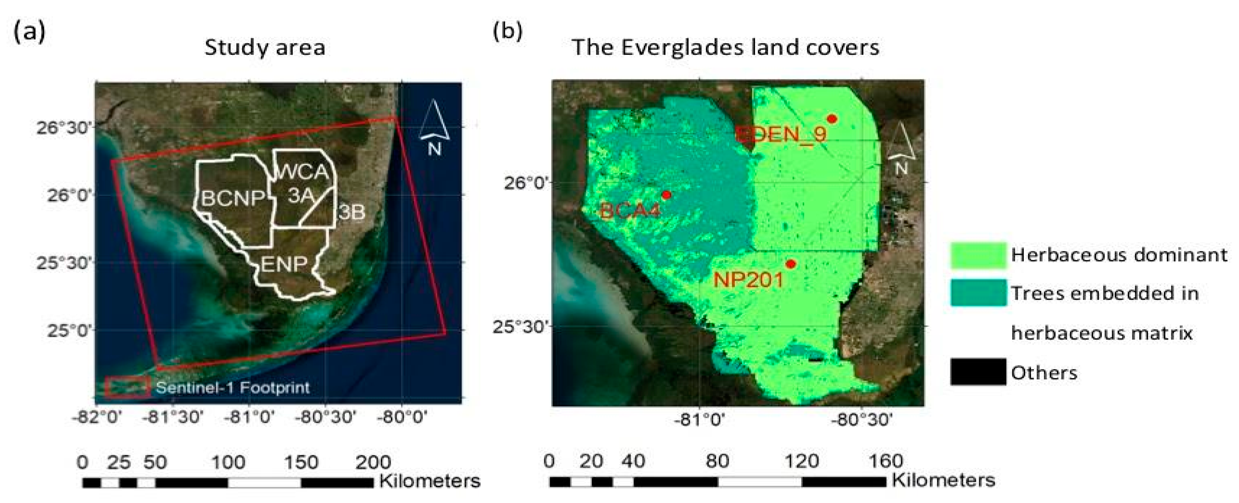
SAR backscatter acquired over wetlands is affected by vegetation biophysical parameters and hydrological conditions. Previous studies have found that C-band co-polarized backscatter changes, over time, often reflect seasonal hydrological variations [1,25,28,29]. The relationships between C-band backscatter and water depth were described using different types of linear models, according to vegetation characteristics [1,25,26,27,28,29,30,40]. This section introduces the current knowledge of C-band backscatter behavior, in response to changes in water depths, for three major wetland vegetation types: open-canopy woody, medium-dense herbaceous, and sparse herbaceous (Figure 1). Woody and herbaceous vegetation with dense canopies are not discussed because backscatter is insensitive to changes in hydrological conditions of the ground substrate, and only a small portion of C-band microwave energy can be transmitted through the canopies.

The types of linear relationships between C-band σ° and d_w vary among vegetation types. For open-canopy woody vegetation, water-depth increase enhances double-bounce scattering (Figure 1a,b), resulting in linearly increasing backscatter (Figure 1c) [1,25]. For medium-dense herbaceous vegetation, under the condition of shallow water depths, relative to plant heights, backscatter increases with water depth, due to enhanced double-bounce (Figure 1e) [41]. However, after water depth reaches a certain level, backscatter decreases with increasing water depth, because an increasing portion of the microwave energy scatters away from the satellite (Figure 1f). Consequently, the σ°-d_w relationship is a combined positive and negative linear relationship (Figure 1g) [25]. For sparse herbaceous vegetation, increasing water depth leads to decreased backscatter because emergent vegetation volume decreases (Figure 1i,j), resulting in negative linear relationships between σ° and d_w (Figure 1k) [25,28,29].

The linear σ°-d_w relationships provide the foundation for backscatter-based SWDI detection, which assumes that change in water-depth is the main factor for backscatter variations for a given vegetation type. The difference between pre-event and post-event backscatter values depends on the magnitude of changes in water depth. Reliable SWDI detection requires pre-event conditions to be characterized by standing water because, if unflooded, backscatter is mainly determined by other parameters, such as soil moisture [28]. In addition, pre-event water depths should not be higher than the plants because backscatter from fully submerged vegetation is insensitive to further water-depth increases due to specular reflection. Under shallow water-depth conditions, relative to plant heights, i.e., with a portion of plant volume emerging from water surfaces, backscatter is likely sensitive to water-depth increases. Additionally, if a SAR observation is acquired during a hurricane event, winds could change the horizontal and vertical plant structure, and it is important to evaluate wind effect on backscatter changes.

Our SWDI detection only relied on the negative and combined positive–negative σ°-d_w linear relationships for herbaceous vegetation, assuming that backscatter decreases in response to water-depth increases (Figure 1h,l). Note that, in the cases of combined linear relationships, this assumption is valid only when the pre-event water depth is around the ‘hinge’ area, where the positive and negative linear relationships transition or the water depth is even deeper and corresponds to the negative linear trend (Figure 1h). The SWDI detection did not rely on the positive σ°-d_w linear relationships for woody vegetation because C-band energy is less sensitive to changes in hydrologic conditions than herbaceous vegetation [7,25]. The low sensitivity is attributed to the low transmission of microwave energy through woody canopies [25].

2.2. Study Area

Our study area is a part of the greater Everglades wetland ecosystem in south Florida (Figure 2a). The greater Everglades ecosystem is characterized by a small topographic gradient of 2 cm per kilometer [7] and is subject to subtropical climate, with seasonal rainfall. The study area was set to the extent of water surface maps, generated by the Everglades Depth Estimation Network (EDEN), as reference data for validating SWDI detection. The study area consists of hydrologically controlled- and natural-flow units (Figure 2a). The hydrologically controlled areas include two Water Conservation Areas (WCA3A and WCA3B), and the natural flow areas include Everglades National Park (ENP) and Big Cypress National Preserve (BCNP). The vegetation types in WCAs and ENP are dominated by herbaceous marshes and prairies, sloughs, and woodlands with trees and shrubs (Figure 2b) [42]. BCNP is dominated by ‘trees embedded in herbaceous matrix’ land cover, representing areas with sparse to dense tree covers, mainly bald cypress (Taxodium distichum), within the matrix of herbaceous species that often form the understory [43]. Around one-quarter of BCNP is covered with treeless wet prairies and marshes (Figure 2b) [43].

2.3. Hurricane Irma

Hurricane Irma was one of the strongest hurricanes to hit the eastern US coast on record. It made landfall in the southern Florida Keys, on 10 September 2017, as a catastrophic hurricane category four on the Saffir–Simpson hurricane wind scale, with maximum sustained winds of ~58 m/s, continued northward as a category three hurricane, arrived near Naples, Florida, later, on the same day, with maximum sustained wind speed of ~51 m/s [44,45]. The strongest observed wind gust was 64 m/s, which was recorded near Naples [46]. Hurricane Irma produced heavy precipitation, resulting in an extensive, rapid, and significant water-depth increase for the Everglades wetlands. The hurricane caused significant damage to vegetation canopies of the coastal mangrove forests along the west coast of the Everglades (not included in the area of interest for this study), whereas the impact on the eastern inland wetlands was not significant [47,48]. After Hurricane Irma’s occurrence, until the end of November, the intensity of occasional rainfall events was much weaker than the rainfall induced by Hurricane Irma, and according to water gauge measurements, water depth gradually decreased to the pre-event levels.

3. Data and Data Preprocessing

This study relied on two multi-temporal datasets: a satellite-based SAR dataset and a ground-based hydrological dataset. The satellite-based dataset consisted of C-band SAR backscatter observations, acquired by the satellite, Sentinel-1A. The hydrological dataset consisted of gauge measurements of water depths from the EDEN network and interpolated water surface maps [49,50].

3.1. SAR Data and Pre-Processing

Sentinel-1A data were consistently acquired for the Everglades, with 51 scenes, from September 2016 to September 2018 (one year before and one year after Hurricane Irma), from the same ascending path 48 (European Space Agency-https://scihub.copernicus.eu/dhus/#/home, last accessed on 12 December 2021). SWDI detection used a total of nine acquisitions in the year 2017: three pre-event ones, acquired on 24 July, 17 and 29 August, one during-event, on 10 September, and five post-event ones, on 4, 16, 28 October, and 9 and 21 November. The three pre-event SAR dates formed a baseline to capture the rapid water-depth increase induced by Hurricane Irma, with their water-depth maps presented in Section 5.2. The rest of the SAR data were used to illustrate the σ°-d_w relationships (Section 5.1).

This study used Sentinel-1 Level-1 high-resolution Ground Range Detected (GRD) Interferometric Wide (IW) mode products that included C-band VV and VH data (C-VV and C-VH), with a spatial resolution of 20 m and 22 m in range and azimuth directions, respectively. Sentinel-1A data processing used the Sentinel Application Platform (SNAP), provided by ESA. The processing included thermal noise removal, radiometric calibration, speckle filtering, and terrain correction using the 3-arcsecond Shuttle Radar Topography Mission (SRTM) DTM. Backscatter was expressed as sigma naught (σ°) in decibel (dB) units and resampled to 20-m pixel spacing using bilinear interpolation. This procedure generated two co-registered stacks of backscatter time series in C-VV and C-VH, respectively. However, this study does not emphasize the C-VH data because of noisy pre-event backscatter and anomalous during-event backscatter values, possibly due to backscatter from waves induced by winds.

3.2. Hydrologic Data and Digital Terrain Model

Hydrologic data, including water gauge measurements and water surface maps, and DTM data, were provided by EDEN (https://sofia.usgs.gov/eden/, last accessed on 16 November 2021). Daily median water gauge measurements were used to relate to the daily interpolated surface maps. For 10 September 2017, during the passage of Hurricane Irma over south Florida, hourly water level data were used because of rapid water-level increases, induced by heavy rainfall. The hourly water level measurements were from 19:00–20:00 Eastern Standard Time (or UTC 23:00–24:00), corresponding to the Sentinel-1 acquisition time (UTC 23:27). We subtracted the ground elevation value from water level measurements for each water gauge to calculate the water depth time series.

EDEN daily water surface maps represent median water levels, with a vertical accuracy of 3.3 cm, and align with the same grid, with a 400 m × 400 m resolution [49,50]. We obtained daily median water surface maps, corresponding to eight of the nine Sentinel-1 acquisition dates (three pre-event and five post-event) used for SWDI detection, and, for the during-event date, the hourly water surface map for UTC 23:00–24:00, interpolated by hourly water gauge measurement [51], was used because of rapid water-depth increases during Hurricane Irma. The hourly surface interpolation method was the same as other daily median maps, using the radial basis function (RBF) and multi-quadric method [49,50,51,52]. Similarly, the EDEN DTM map was subtracted from water surface maps to generate water-depth maps.

4. Methodology

We developed an SWDI detection algorithm that classifies SWDI and non-SWDI areas with respect to baseline hydrological conditions for each of the six target SAR dates (one during- and five post-event). The algorithm classifies 400-m resolution pixels of the regular EDEN grid into three classes ‘SWDI’, ‘Non-SWDI’, and ‘Uncertain’. This section mainly describes the backscatter-based SWDI detection algorithm consisting of three stages (Figure 3, Section 4.1). Section 4.2 describes the selection of values for threshold parameters used in the algorithm.

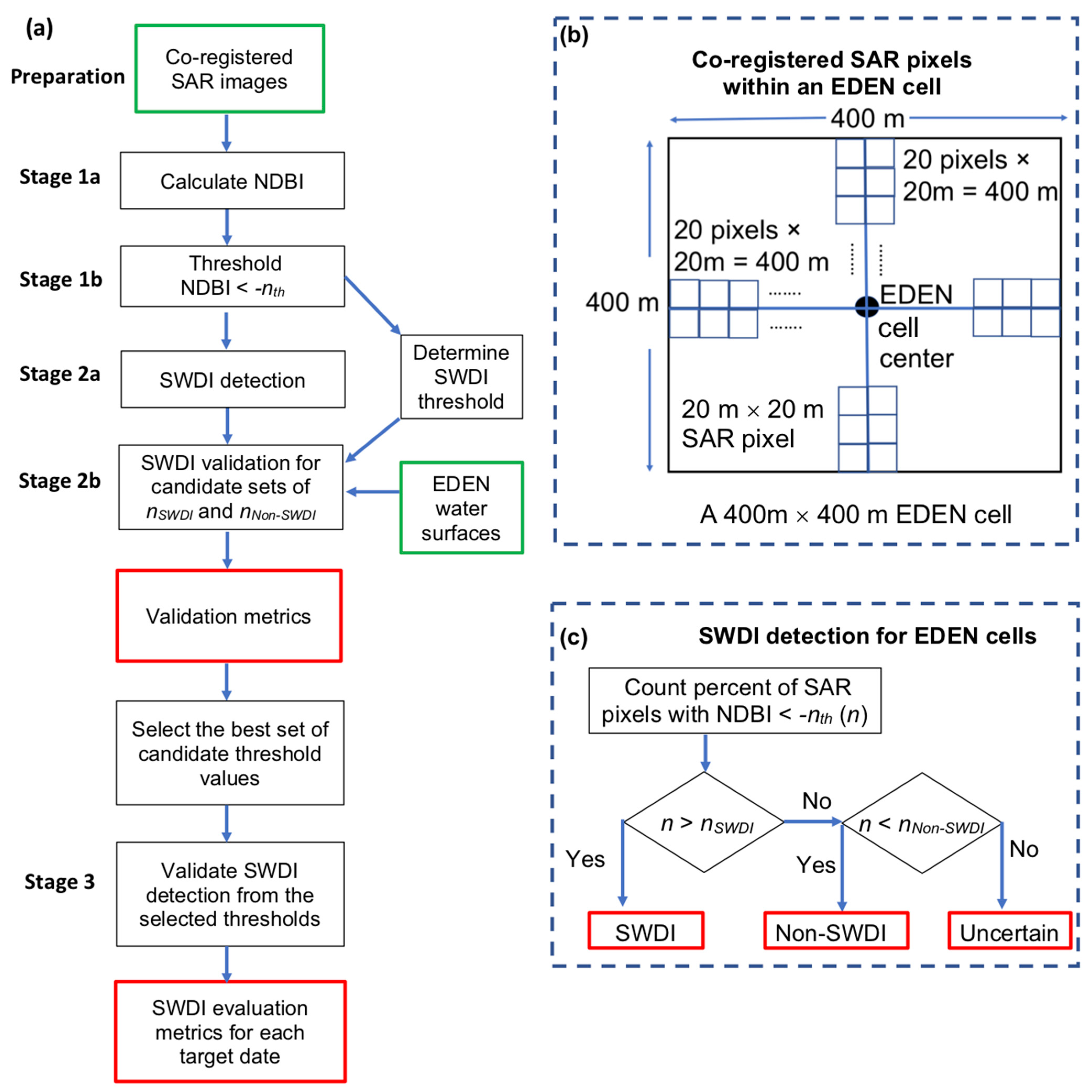
4.1. SWDI Detection Methodology

Our SWDI detection was based on two assumptions: (1) water depth is the factor controlling most of the variations in backscatter, and (2) SWDI leads to backscatter decreases for herbaceous wetlands because they are characterized by negative or combined σ°-d_w linear relationships depending on vegetation density (Figure 1). The first assumption is valid for major vegetation types in the Everglades under flooded conditions [25], whereas it may not hold under unflooded (groundwater) conditions. We, therefore, examined the flooding conditions for the selected SAR dates, especially for three pre-event dates when water levels are lower than the during- and post-event dates (Section 5.2). In addition, we evaluated Hurricane Irma’s wind impact on backscatter values by selecting 135 water gauges, for which water depth measurements were available for the period of interest (September 2016–September 2018) to calculate σ°-d_w linear models based on the methodology described by Zhang et al. [25]. For each water gauge, the during-event backscatter’s deviation from the linear model was calculated (Figure S1a,b) and compared to the Mean Absolute Error (MAE) of the linear model, which is the average absolute deviation value for all SAR observations used for the linear model.

The second assumption does not hold for combined σ°-d_w linear relationships if pre-event water depths are shallow relative to plant heights when SWDI leads to backscatter increase instead of decrease (Figure 1h). To verify the second assumption, we classified EDEN water gauge pixel locations into four classes (positive, combined positive–negative, negative (each with strong correlations with R² > 0.5 and p-value < 0.04), and weak linear σ°-d_w relationships) by applying the classification method provided by Zhang et al. [25] on the two-year backscatter and water depth time series. For the gauge pixels with a combined positive–negative linear relationship, their relative pre-event water depths were investigated and are shown in Figure S2.

If both assumptions are verified, SWDI detection mainly uses a Normalized Difference Backscatter Index (NDBI) that calculates mean and standard deviation values for pre-event backscatter [10,53]. The SWDI detection algorithm consists of a data preparation step and three stages (Figure 3a): NDBI calculation and thresholding (Stage 1), SWDI detection and validation using candidate sets of thresholds (Stage 2), and detailed validation of SWDI detection resulting from the selected set of thresholds (Stage 3).

Data Preparation. The SWDI detection unit was set to the EDEN water surface maps’ 400 m × 400 m grid cell. The 20-m SAR pixels were co-registered to fit into the EDEN grid (Figure 3b) by first resampling the EDEN grid into a 20-m resolution grid as an intermediate product and then resampling the nine selected SAR images to this grid. As a result, each 400-m EDEN cell contained 400 (20 × 20) co-registered SAR pixels (Figure 3b).

Stage 1 includes NDBI calculation (Stage 1a) and thresholding to select SAR pixels likely to have SWDI (Stage 1b). The analysis is conducted at a 20-m SAR pixel scale.

Stage 1a calculates NDBI for each SAR pixel with Equation (1) using three pre-event and one target date (during or post-event) backscatter values. NDBI is the normalized difference value between target and pre-event mean backscatter.

$$NDBI=\frac{\sigma {°}_t-\overline{\sigma {°}_p }}{S{D}_p}$$

(1)

where $\sigma {°}_t$ denotes backscatter for a target image pixel, $\overline{\sigma {°}_p}$ denotes the average of three pre-event backscatter values as backscatter baseline, $S{D}_p$ =$\sqrt{\frac{1}{3}{\displaystyle \sum }_{\mathrm{i}=1}^3{\left(\sigma {°}_{pi}-\overline{\sigma {°}_p}\right)}^2}$ denotes the standard deviation of the pre-event backscatter, with ${\sigma }_{pi}^o$ denoting a pre-event backscatter.

Based on the linear σ°-d_w relationships described in Section 2.1, differences between $\sigma {°}_t$ and $\overline{\sigma {°}_p}$ are proportional to changes in water depths. $S{D}_p$ accounts for pre-event backscatter variations, and large $S{D}_p$ reduces the confidence of SWDI detection.

Stage 1b thresholds NDBI values using a criterion of NDBI < -n_th, with the rationale that water-depth increase leads to backscatter decrease because of negative or combined σ°-d_w linear relationships for herbaceous vegetation. Significant water-depth increase leads to negative NDBI values with large magnitudes. For example, using an n_th of 3, i.e., a threshold criterion as NDBI < −3, indicates that the normalized change between the baseline and target backscatter is more negative than −3. Based on the NDBI threshold n_th, we determine the SWDI detection threshold as n_th times the pre-event water-depth standard deviation (Figure 3a), according to the linear σ°-d_w relationships.

We mapped the NDBI with three classes: NDBI < −n_th, −n_th <= NDBI <= n_th, and NDBI > n_th to spatially investigate the pixels that were likely to have SWDI. Though the algorithm does not use positive NDBI values as an indicator for SWDI, i.e., NDBI > n_th, due to weak correlations between σ° and d_w for woody vegetation (Section 2.1), we mapped this class to further justify that the NDBI > n_th criterion should not be used in SWDI detection.

Stage 2 consists of SWDI detection (Stage 2a) and validation (Stage 2b), and it is conducted at a 400-m EDEN cell scale. Stage 2a describes the SWDI detection algorithm, and Stage 2b describes the metrics for validating SWDI detection results.

Stage 2a analyzes NDBI values resulting from Stage 1 to classify each EDEN cell into one of three classes: ‘SWDI’, ‘Non-SWDI’, and ‘Uncertain’ (Figure 3c). ‘SWDI’ class indicates that water-depth increase relative to the baseline is higher than the SWDI detection threshold (determined in Stage 1b); ‘Non-SWDI’ class indicates that water-depth increase is less than the threshold; ‘Uncertain’ class indicates that the status of water-depth change could not be determined.

The algorithm first calculates a term n, the percentage of SAR pixels contained in an EDEN cell with NDBI < -n_th, meaning, for that SAR pixel, the backscatter change from baseline to the target, after normalization (see Equation (1)), is more negative than -n_th. The algorithm then compares n to two threshold parameters: n_Non-SWDI and n_SWDI, (with n_Non-SWDI ≤ n_SWDI). The EDEN cell is classified as ‘SWDI’ when n > n_SWDI; ‘Non-SWDI’ class when n < n_Non-SWDI; ‘Uncertain’ class when n_Non-SWDI ≤ n ≤ n_SWDI. (For example, n_Non-SWDI = 10% and n_SWDI = 20%; the rationale for searching of optimal values is explained later in Stage 2b). The EDEN cell would be classified as ‘SWDI’ when n > n_SWDI, meaning if there is a high percentage of SAR pixels with NDBI < -n_th, it is likely for SWDI to occur at that EDEN cell. On the other hand, the EDEN cell would be classified as ‘Non-SWDI’ class when n < n_Non-SWDI. When a low percentage of SAR pixels satisfy NDBI < −n_th, the observed NDBI values are assumed to primarily come from noisy backscatter values, and it is inferred that SWDI does not occur in that pixel (non-SWDI). Finally, when n_Non-SWDI ≤ n ≤ n_SWDI, the pixel would be classified as ‘Uncertain’ class.

Stage 2b systematically validates SWDI detection resulting from candidate values of n_SWDI and n_Non-SWDI to select the set of thresholds that yields the best performance on detection. We systematically tested n_SWDI and n_Non-SWDI candidates with a range from 0% to 100% (note that n_Non-SWDI ≤ n_SWDI) and an increment of 5%. Detection results were compared to reference water-depth increase maps produced for each target date by subtracting the baseline from a target water surface, with each reference map including ‘SWDI’ and ‘Non-SWDI’ classes determined by the SWDI detection threshold (Figure 3a). For each set of candidate thresholds, metrics were calculated, including overall accuracy (OA), Kappa coefficient [54], and the average percentage of the ‘Uncertain’ class for six target dates as a whole, to select the set with high accuracy but low ‘Uncertain’ class percentage.

Stage 3 is a detailed validation for SWDI detection resulting from the selected set of thresholds with the best performance. We generated an evaluation map for each target SAR date with five classes, including correctly classified (‘True SWDI’ and ‘True Non-SWDI’), incorrectly classified (‘False SWDI’ and ‘False Non-SWDI’), and ‘Uncertain’. Evaluation metrics were tabulated, including the percentage of each class, OA, Kappa coefficient, user’s and producer’s accuracy (UA and PA) for ‘SWDI’ and ‘Non-SWDI’ classes. We also compared OA among different land covers for each target date.

4.2. Selection of Threshold Values

An initial threshold n_th of 3 was used to classify NDBI values based on previous studies using a similar technique for hydrological applications [10,17]. A sensitivity test was conducted using n_th of 2 and a corresponding SWDI detection threshold of 8 cm (2 × 4 cm) to investigate SWDI detection accuracy. SWDI detection threshold is n_th times the pre-event water-depth standard deviation. The standard deviation map showed a range of 4 ± 2 cm for most of the study area (84%, Section 5.2) and, therefore, we used the spatial mean value of standard deviations, 4 cm, to represent the standard deviation for the study area, resulting in an SWDI detection threshold as n_th × 4 = 12 cm. Another sensitivity test was conducted using different values ranging from 2 to 6 cm to represent the pre-event water-depth standard deviation for the entire study area.

5. Results

This section includes three parts. The first section presents the three types of σ°-d_w linear relationships (Section 5.1), which serves as foundations for SWDI detection. The second section presents pre-event hydrologic conditions (Section 5.2). Finally, Section 5.3 consists of three subsections, following three stages of the algorithm.

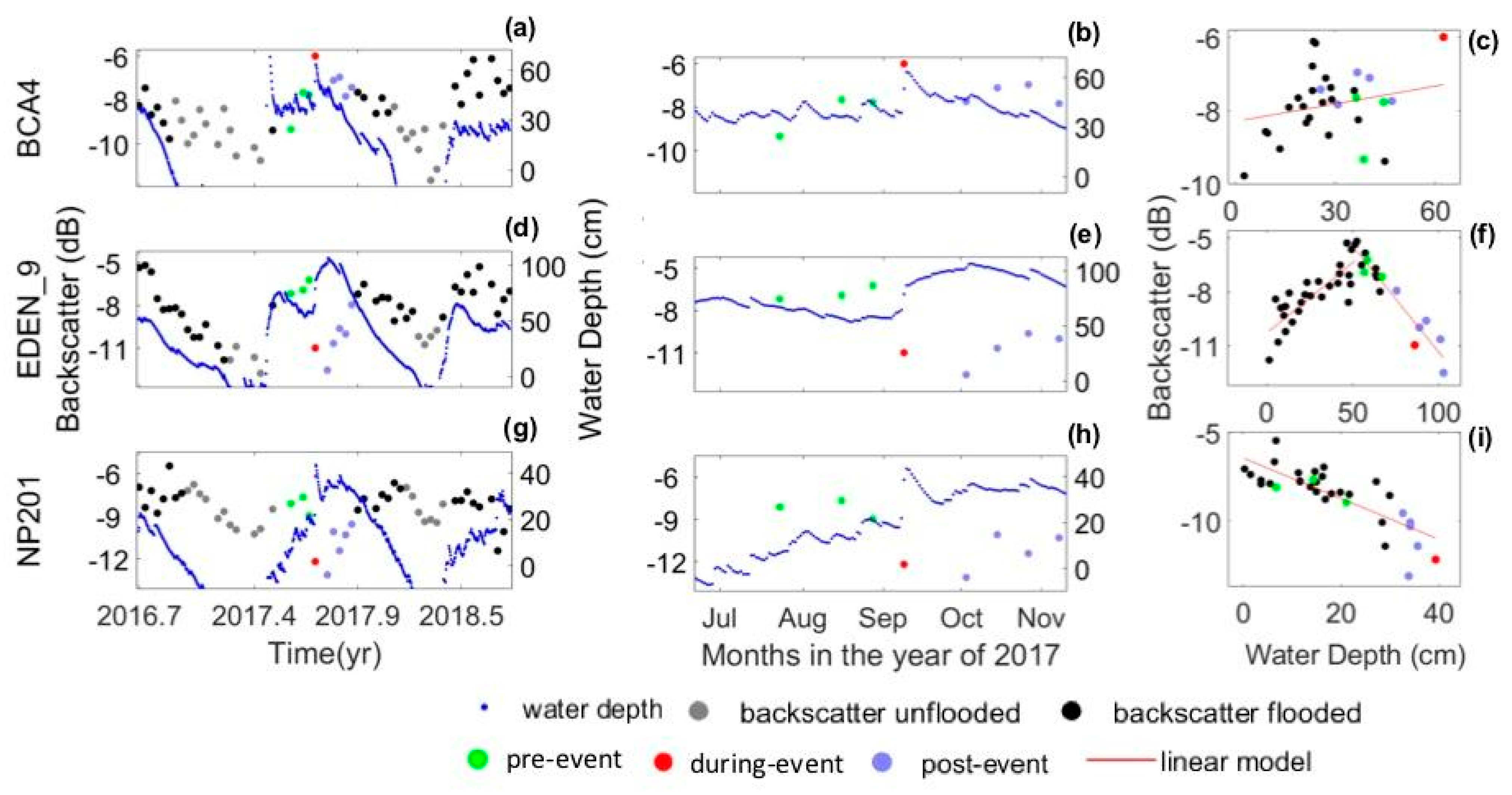
5.1. Backscatter Behavior in Response to Variations in Water Depth for Three Selected Water Gauges

Three representative gauges were selected to illustrate the three types of σ°-d_w linear relationships (Section 2.1); ‘BCA4’, ‘EDEN_9’, and ‘NP201’ (Figure 4). Gauge ‘BCA4’ was located within cypress swamps in BCNP, and ‘EDEN_9’ and ‘NP201’ were located in graminoid marshes in WCA-3A and ENP, respectively (Figure 2b). The water gauges exemplified positive, combined positive–negative, and negative σ°-d_w relationships, respectively. The presented backscatter values were obtained by using the SAR pixel containing the gauge location.

For water gauge ‘BCA4’, backscatter was in phase with water-depth variations (Figure 4a). The positive linear σ°-d_w relationship was weak (R² = 0.04, Figure 4c). During-event backscatter was higher than all pre- and post-event backscatter values, and the during-event water depth was also higher than the other dates (Figure 4b).

For water gauge ‘EDEN_9’, backscatter was in phase with water-depth variations at low water depths (Figure 4d). However, backscatter was out of phase with water-depth variations during the highlighted period with high water depths (Figure 4e). The scatter plot of backscatter and water depth showed a combined positive and negative σ°-d_w linear relationship (R² values are 0.68 and 0.91, respectively, Figure 4f). The during-event backscatter was lower than the pre-event backscatter values, whereas the during-event water depth was higher (Figure 4e). Post-event SAR dates showed gradually decreasing water depths and increasing backscatter values.

For the ‘NP201’ water gauge, backscatter and water-depth variations were out of phase for the entire time series (Figure 4g). The scatter plot of backscatter and water depths showed a negative σ°-d_w linear relationship with an R² of 0.62 (Figure 4i). The during-event date showed a higher water depth and lower backscatter value than the pre-event ones. Post-event backscatter increased as water depths decreased (Figure 4h).

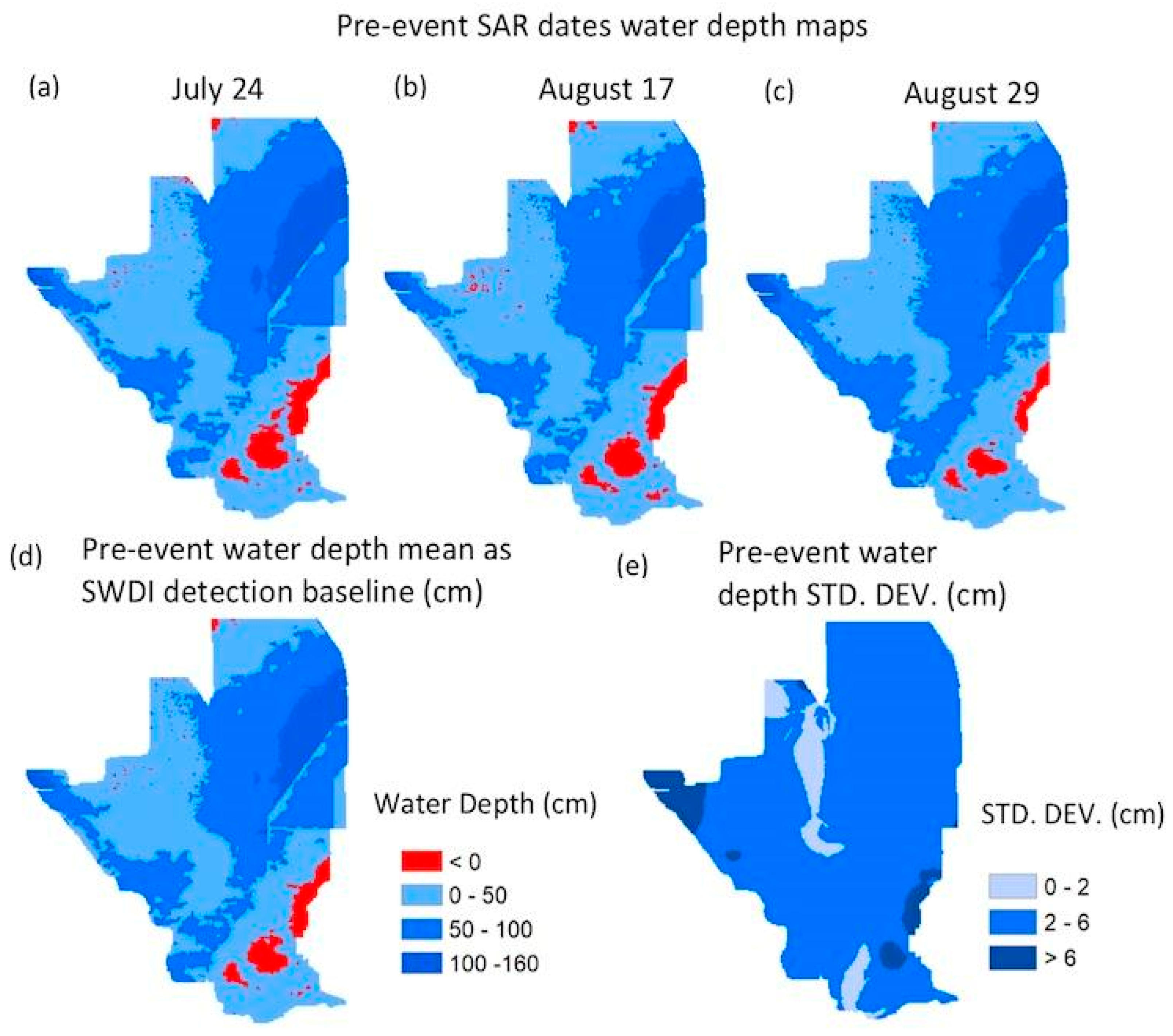
5.2. Pre-Event Hydrological Conditions

We investigated pre-event hydrological conditions to verify the first assumption, that water depth is the factor controlling most of the variations in backscatter from vegetated wetlands, which is not valid under unflooded conditions. The water-depth maps, derived from EDEN’s water surface maps, for the three pre-event SAR acquisition dates (24 July, 17 and 29 August in 2017), revealed that most of the study area was flooded with water depths of less than 100 cm (Figure 5a–c). Though water-depth maps were missing for the northwestern BCNP, due to the lack of DTM, EDEN water gauges in BCNP indicated flooded conditions during the pre-event dates. Because the study area mainly consists of woody vegetation in BCNP and herbaceous vegetation, dominated by tall species (e.g., Cladium jamaicense, with heights over 160 cm) in WCAs and ENP [55,56], a significant portion of plant volume emerged above the water surface. Consequently, the pre-event dates were characterized by flooded conditions, and soil moisture makes little contribution to backscatter, supporting the first assumption that changes in backscatter are mostly controlled by water-depth variations.

During-event backscatter’s deviations from linear models were compared to MAE for 135 selected water gauges, and most of the gauges showed during-event backscatter deviations were at a similar level to the MAE, i.e., less than 2 dB (Figure S1), indicating that the hurricane’s wind did not have a significant impact on the during-event backscatter values. Therefore, the first assumption proved to be valid. Details of evaluating Hurricane Irma’s impact on during-event backscatter values is presented in Note 2.

To verify the second assumption, that SWDI leads to backscatter decreases for medium–dense herbaceous vegetation, characterized by combined σ°-d_w linear relationships, we classified σ°-d_w relationships for water gauges and selected eleven gauges as combined positive–negative relationships (Figure S2). Their pre-event water depths were either located in the “hinge” area or along with the negative linear trend on the σ°-d_w scatter plots (Figure S2 and Figure 4f). The eleven selected water gauges are widely distributed in WCAs and ENP and, therefore, well represent the medium–dense herbaceous vegetation (Figure S3). The results verified the second assumption of backscatter decreases in response to SWDI for medium–dense herbaceous vegetation.

5.3. Results of SWDI Detection and Validation

5.3.1. NDBI Maps for the During- and Selected Post-Event SAR Dates

NDBI maps were generated for the Everglades wetlands, including BCNP, WCAs, and ENP (Figure 2a). Though the proposed SWDI methodology cannot be applied to forested vegetation, we included the BCNP region, where cypress trees are often embedded within the herbaceous vegetation matrix. Because we used a 400-m scale SWDI detection unit, the herbaceous vegetation could provide useful NDBI values for the SWDI detection.

We selectively present three NDBI maps, resulting from methodology stage 1, including the during-event and two post-event dates (4 October and 21 November) (Figure 6). The rest of the post-event NDBI maps are presented in Supplementary Material Figure S4, which look similar to the November 21 map in Figure 6c. The during-event NDBI values were less than −3 (n_th = 3) for most of WCAs and ENP (blue areas in Figure 6a), whereas NDBI values were larger than 3 for BCNP (red areas) and boundary area between WCA-3A and 3B.

The NDBI map of the first post-event date, 4 October, was similar to the during-event map, showing most ENP and WCAs with NDBI values less than −3, whereas, for BCNP, the areas with NDBI values larger than 3 were much smaller than during-event. The boundary area between WCA-3A and 3B showed negative NDBI values. The NDBI map of the last post-event date showed that WCAs and north ENP were dominated by NDBI values less than 3, whereas BCNP was dominated by NDBI values larger than 3.

To illustrate the contrast pattern of NDBI values between woody and herbaceous vegetation, we selected three local areas for the during-event day under SWDI conditions (Figure 6(a1–a6)). The first area, located in WCA-3B, was characterized by tree islands and surrounding sloughs with sparse sawgrass (Figure 6(a1,a2)); the second area, located in BCNP, was characterized by mixed tree species forests (Figure 6(a3,a4)); the third area was pine rockland, with elevated ground surfaces (Figure 6(a5,a6)). All three areas showed that woody vegetation had positive NDBI values, whereas surrounding herbaceous vegetation had negative values.

5.3.2. SWDI Detection and Validation Using Candidate Sets of n_SWDI and n_Non-SWDI Thresholds

SWDI detection and validation were conducted based on NDBI values, using the methods described in stage 2 of the Methodology section. SWDI validation metrics, resulting from candidate sets of threshold parameters n_SWDI and n_Non-SWDI, were sorted according to the Kappa coefficient (

Table 1. SWDI detection candidate sets of thresholds and three validation metrics. The row in bold font indicates the optimal set of thresholds.

nSWDI (%)	nNon-SWDI (%)	Overall Accuracy	Kappa Coefficient	Average Uncertain Pixels Percentage
45	10	0.81	0.60	0.30
40	10	0.81	0.60	0.27
35	10	0.81	0.60	0.24
50	10	0.80	0.60	0.32
30	10	0.81	0.59	0.21
25	10	0.81	0.58	0.17
20	10	0.81	0.57	0.13
35	15	0.78	0.55	0.17
40	15	0.78	0.55	0.20
45	15	0.77	0.54	0.22
30	15	0.78	0.54	0.14
50	15	0.77	0.54	0.25

). Further, n_SWDI values higher than 45% were removed from Table 1 because of high ‘Uncertain’ class percentages. The top candidate set had n_SWDI of 45% and n_Non-SWDI of 10%, resulting in a Kappa coefficient of 0.59, an overall accuracy of 0.8, and an ‘Uncertain’ class percentage of 30% (Table 1). The top seven candidate sets had the same n_Non-SWDI value of 10%, and the five following sets had a value of 15%. The set with n_SWDI of 20% and n_Non-SWDI of 10% resulted in the lowest ‘Uncertain’ class percentage and moderate overall accuracy and Kappa coefficient. Considering the trade-off between accuracy and ‘Uncertain’ class percentage, we selected the optimal set with n_SWDI = 20% and n_Non-SWDI = 10% for further analyses.

We tested using the ‘NDBI > n_th or NDBI < −n_th’ criterion for SWDI detection and validation, which resulted in lower accuracy than the ‘NDBI < −n_th’ criterion (Table S1). In addition, a sensitivity test was conducted using n_th of 2 with a corresponding SWDI detection threshold of 8 cm, resulting in similar accuracy to n_th of 3 (with the detection threshold of 12 cm), and the selected set (n_SWDI = 20% and n_Non-SWDI = 10%) also achieved a high accuracy and low percentage of ‘Uncertain’ class (Table S2). We also present the validation metrics resulting from C-VH data (Table S3), which had lower Kappa coefficients than those of C-VV.

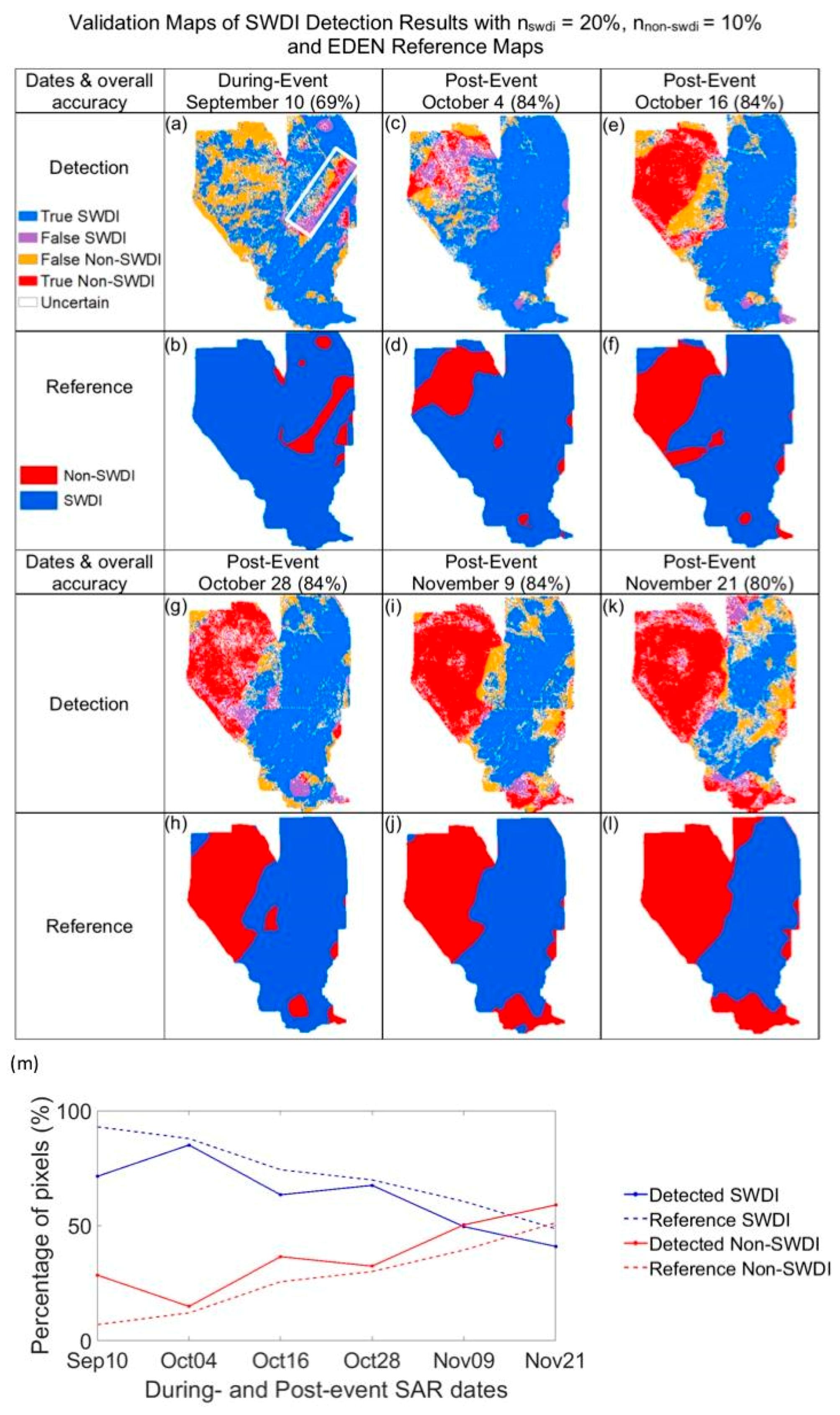
5.3.3. SWDI Validation Using the Selected Set of Thresholds

SWDI validation maps and EDEN reference maps are presented for each of the six target dates (Figure 7a–l), resulting from the selected set of thresholds (n_SWDI = 20% and n_Non-SWDI = 10%). The validation map for the during-event date showed ‘True SWDI’ areas for most ENP and WCAs and ‘False Non-SWDI’ areas in BCNP (Figure 7a). Boundary areas between WCA-3A and 3B showed a mix of true and false classifications.

The post-event dates featured large areas of true classifications, for both SWDI and non-SWDI classes, including northern ENP, WCA-3A, and 3B with dominant SWDI class, and progressive expansion of non-SWDI extents from BCNP to northwestern ENP (Figure 7c–l). Another noticeable feature was the expansion of non-SWDI extents at the southern tip of ENP for the last three target dates. However, an extensive eastern part of the study area showed false classification for the last date, November 21 (Figure 7k).

Temporal variations of the percentages of SWDI and non-SWDI classes were highly consistent between classification and reference data (Figure 7m). For the during-event day, the SWDI percentage was the highest, and the non-SWDI percentage was the lowest. For the post-event days, SWDI percentages progressively decreased, and non-SWDI areas increased. For the last post-event date, the non-SWDI percentage exceeded the SWDI percentage, for both classification and reference data.

Daily evaluation metrics (

Table 2. SWDI validation metrics based on the selected set of thresholds with n_SWDI = 20% and n_Non-SWDI = 10%. ‘Uncertain’ class was not taken into account when calculating other accuracy metrics. The percentages of the first four classes (True SWDI, False SWDI, False Non-SWDI, and True Non-SWDI) add up to 100%.

Date	True SWDI	False SWDI	False Non- SWDI	True Non- SWDI	Uncertain	OA	Kappa	SWDI		Non-SWDI
								UA	PA	UA	PA
20170910	0.67	0.05	0.26	0.02	0.12	0.69	0.03	0.94	0.72	0.08	0.50
20171004	0.79	0.06	0.09	0.06	0.11	0.84	0.33	0.92	0.89	0.38	0.47
20171016	0.61	0.02	0.13	0.24	0.10	0.84	0.64	0.96	0.82	0.64	0.91
20171028	0.61	0.07	0.09	0.23	0.13	0.84	0.63	0.90	0.87	0.72	0.77
20171109	0.47	0.03	0.13	0.37	0.12	0.84	0.67	0.94	0.77	0.73	0.93
20171121	0.35	0.06	0.14	0.45	0.18	0.80	0.59	0.84	0.71	0.76	0.88

) showed that the ‘True SWDI’ class percentage decreases with time, whereas the ‘True Non-SWDI’ percentage increases with time. False classes had low percentages for all dates, except for the ‘False Non-SWDI’ class in the during-event date (26%). Percentages of the ‘Uncertain’ class were less than 20% for each target date. Overall accuracies were above 80% for all post-event dates, but only 69% for the during-event date. Similarly, Kappa coefficients were around 0.6 for the last four post-event dates, but only 0.03 and 0.33 for the first two dates, respectively. The first two dates showed user’s and producer’s accuracies for the non-SWDI class no greater than 0.5. In contrast, the remaining post-event dates showed high user’s and producer’s accuracies, for both SWDI and non-SWDI classes.

We compared the overall accuracies between ‘herbaceous dominant’ and ‘trees embedded in herbaceous matrix’ (

Table 3. Overall accuracy of SWDI detection for two major land cover types.

	September 10	October 4	October 16	October 28	November 9	November 21
Herbaceous dominant	0.79	0.94	0.92	0.89	0.85	0.75
Trees embedded in herbaceous matrix	0.40	0.61	0.68	0.75	0.82	0.90

). The herbaceous area had high accuracy throughout the time series, whereas ‘trees embedded in herbaceous matrix’ land cover had low accuracy for the during-event date but higher accuracy for the post-event dates. In addition, SWDI detection results, using C-VH data with the selected set of thresholds (n_SWDI = 20% and n_Non-SWDI = 10%) (Table S4), showed lower accuracy than C-VV for all six dates. The sensitivity test using different values (2 to 6 cm) to represent the study area’s pre-event water-depth standard deviation showed that the initial chosen value of 4 cm achieved the best overall accuracy for SWDI detection (Table S5).

6. Discussion

This study developed a backscatter-based algorithm to map SWDI and non-SWDI areas associated with severe rainfall events in wetlands. We tested the algorithm using the Everglades wetlands as an example, which experienced heavy rainfall and rapid water-depth increase during the passage of Hurricane Irma, in September 2017. We used pre-event water surface as a baseline, one during-event, and five post-event SAR dates as targets. The algorithm was conducted at a 400-m scale and classified EDEN cells into three classes: ‘SWDI’, ‘Non-SWDI’, and ‘Uncertain’, which were validated using EDEN’s water-surface products as reference. The algorithm accurately detected extensive SWDI areas during the event and progressive expansion of non-SWDI areas where water depths dropped close to pre-event conditions within two months.

This section consists of three subsections. Section 6.1 evaluates the performance of the SWDI detection method, based on the results from each stage of the methodology. Section 6.2 discusses the conditions and limitations of the algorithm applications. Section 6.3 compares this study to previous SAR and InSAR-based studies that detect changes in hydrological conditions.

6.1. Evaluation of SWDI Detection Algorithm Performance

Section 6.1 includes three parts, according to three stages of the methodology: (1) evaluating NDBI thresholding; (2) discussing the selection of thresholds n_SWDI and n_Non-SWDI; (3) evaluating SWDI performance, based on validation results generated from the selected set of thresholds.

6.1.1. NDBI Thresholding for SAR Pixels

The first step of the SWDI detection algorithm is to threshold NDBI values at the SAR-pixel scale, which used the criterion of ‘NDBI < −n_th’ (n_th was initially set as 3) by assuming that SWDI results in backscatter decrease for herbaceous vegetation. The results (Figure 6a–c) indicated that for the during- and selected post-event dates, areas with NDBI < −3 were correctly classified as SWDI, according to the validation maps (Figure 7a,c,k). Hence, we concluded that the ‘NDBI < −3’ criterion correctly represents the status of SWDI.

Though positive σ°-d_w relationships have been found for woody wetlands in previous studies [1,25], this study indicates that NDBI > n_th criterion is unreliable for SWDI detection. Although the during-event NDBI map showed extensive areas in BCNP with NDBI > 3 (Figure 6a), correctly represented SWDI conditions according to the reference map (Figure 7b), NDBI > 3 areas in the last post-event date map (Figure 6c) corresponded to non-SWDI conditions (Figure 7l). Adding the criterion of ‘NDBI > n_th’ improved the accuracy for the during-event date but significantly reduced the accuracy for all post-event dates, because of the high ‘False SWDI’ class percentage (Table S1). We attribute it to the weak σ°-d_w linear relationships for woody vegetation, as evidenced by the first water gauge example ‘BCA4’ (Figure 4c), which indicate that biophysical parameters (e.g., canopy cover) can also significantly influence backscatter values, and the assumption that water depth is the main controlling factor on backscatter is not valid.

6.1.2. Selection of SWDI Detection Thresholds

The second step of the methodology conducts SWDI detection using candidate sets of n_SWDI and n_Non-SWDI values and evaluates the detection results on the basis of three metrics: overall accuracy, Kappa coefficient, and the average percentage of ‘Uncertain’ class pixels. The result (Table 1) showed that the threshold n_Non-SWDI must remain at a low level (e.g., 10%) to achieve high accuracy, because high n_Non-SWDI significantly increased the percentage of ‘False Non-SWDI’ class, i.e., classifying an SWDI class pixel into non-SWDI. Consequently, we selected the optimal n_Non-SWDI value of 10% for detecting non-SWDI class.

For the top ten candidate sets in Table 1, with a fixed value of n_Non-SWDI, higher n_SWDI values (e.g., 45% in Table 1) resulted in higher Kappa Coefficients and larger percentages in the ‘Uncertain’ class. Higher n_SWDI led to greater confidence for classifying an EDEN cell as ‘SWDI’ class, but also widened the gap between n_SWDI and n_Non-SWDI values and, therefore, increased the ‘Uncertain’ class percentage. As n_SWDI decreases from 45% to 20%, the ‘Uncertain’ class percentage significantly dropped from 30% to 13%, with little compromise in the Kappa coefficient (Table 1). Considering this trade-off, we selected an n_SWDI of 20% for SWDI detection to achieve high accuracy and a reduced ‘Uncertain’ class percentage.

6.1.3. Evaluating SWDI Performance Based on Validation Results

SWDI validation maps, resulting from the selected set of n_SWDI and n_Non-SWDI thresholds, showed most of the study area was correctly classified for each target SAR date (Figure 7), but with some false classifications at local-scale areas. The false classifications were concentrated at (1) BCNP for the during-event, (2) boundary areas between WCA-3A and 3B for the during-event date, and (3) eastern and northern parts of the study area for the last post-event date. This section explains the reasons for the three types of false classifications.

The first false classification case. For the during-event, a large extent of ‘trees within herbaceous matrix’ land cover in BCNP was classified into the ‘False Non-SWDI’ class (Figure 7a), indicating SWDI condition was incorrectly classified as non-SWDI because the algorithm does not consider positive NDBI values as SWDI. High NDBI values are attributed to deep water surfaces, submerging most of the understory herbaceous vegetation, resulting in significant double-bounce scattering from water surfaces and trunks. The misclassification decreases the user’s and producer’s accuracies for the non-SWDI class (Table 2).

However, the algorithm achieved better performance for the post-event dates in BCNP, since it successfully detected extensive non-SWDI areas with high accuracy (Figure 7c–l, Table 2). Water depths gradually dropped to the pre-event level, and the herbaceous vegetation emerged from water surfaces. The successful detection of non-SWDI areas relies on the herbaceous vegetation within 400-m resolution pixels that provide useful backscatter information for SWDI detection.

Cypress trees in BCNP vary with stature and canopy cover in space, and about half of the cypress swamps consist of open-stand, small cypress trees, embedded in seasonally flooded grassland [43]. A previous study [28] found that open-stand miniature growth cypress sites within the herbaceous matrix in BCNP showed a strong negative correlation (R² = 0.45) between backscatter and water depth, at a 200 m resolution, in contrast to the weak positive σ°-d_w correlations from the ‘BCA4’ water gauge pixel at a 20 m resolution (Figure 4c). Consequently, we suggest that the high SWDI detection accuracy is attributed to the large extents of open-stand small cypress within the herbaceous matrix. However, the water gauges sparsely located in BCNP are not enough to fully evaluate the algorithm’s performance in different characteristics of cypress trees, which can be achieved using a high spatial resolution vegetation map of BCNP in future studies.

The second false classification case. This occurred along the WCA-3A and 3B boundary areas (Figure 7a) for the during-event day. This area is characterized by deep water depths and sparse emergent plants. The results showed positive NDBI values (Figure 6a) because waves induced by the hurricane’s strong winds increased backscatter, which did not reflect variations in water depths. For post-event dates with no strong winds, the algorithm correctly classified this area as the ‘True SWDI’ class. We suggest that the algorithm should not be used on low-cover herbaceous wetlands, under high-wind conditions, because backscatter is primarily affected by scattering from waves.

The third false classification case. ‘False Non-SWDI’ class occurred in the northern and eastern parts of the study area (orange patches in Figure 7k) for the last post-event date. The reference maps showed small ‘Non-SWDI’ areas in both regions (Figure 7l), indicating that water depths dropped close to the baseline level (water-depth increases relative to the baseline are less than 12 cm). A quantitative investigation of the EDEN water surfaces showed that ‘False Non-SWDI’ areas had slightly higher water-depth increases than the SWDI threshold of 12 cm (most of them had less than 17 cm). We suggest that the limited degree of water-depth increase is the main reason for the false classification.

6.2. Conditions and Limitations in Applications of the SWDI Detection Algorithm

The innovative backscatter-based SWDI detection algorithm could be applied to heavy rainfall events in the Everglades, or other wetlands, worldwide. This section discusses the conditions and limitations of the algorithm application.

6.2.1. Conditions of Land Cover Selection

Future studies should mask open water before applying the algorithm because the first assumption, that water depth is the main factor controlling variations in backscatter, does not hold. In addition, the criterion of ‘NDBI < −n_th’ could not be used on forests, though it works with the land cover of trees embedded in the herbaceous vegetation matrix. To monitor ground surface hydrological status for forests, we recommend using L-band backscatter, which is characterized by a higher degree of canopy transmission [1,7], and has been proven to have strong positive linear correlations with water depths in previous studies [26,30].

6.2.2. Conditions of Pre-Event Baseline Data Selection

Previous studies detecting flooded conditions in wetlands often selected many baseline acquisitions for assessing non-flooded conditions [10,17]. In this study, however, the selection of baseline data is more restrictive, because the goal is to separate SWDI and non-SWDI classes, and it should consider flooded conditions, water-depth standard deviations, and relative water depths to plant heights.

First, pre-event baseline selection should avoid unflooded conditions. Backscatter may vary significantly under unflooded conditions due to variations in soil moisture [28]. The first assumption, that only water depth is the main factor controlling variations in backscatter, may not hold under unflooded conditions.

Second, the water-depth standard deviation of the selected pre-event dates should be less than the water-depth increase, induced by the rainfall event of interest, which could be estimated based on water gauge measurements. This study selected three pre-event dates with water-depth standard deviations of about 4 cm (Figure 5e), which is less than the water-depth increase induced by Hurricane Irma, more than 12 cm in most areas (Figure 7b). Significant pre-event water-depth variations result in large variations in backscatter, due to linear relationships between the two variables, and reduce the sensitivity of SWDI detection.

However, under the condition of limited water-depth standard deviation, the number of pre-event SAR acquisitions should be as high as possible, because the backscatter mean ($\overline{\sigma {°}_p}$) and standard deviation ($S{D}_p$) are less susceptible to speckle noise. A large number of pre-event SAR acquisitions could improve SWDI detection performance.

Third, the selection of pre-event dates should examine relative water depths using water gauges with combined positive-negative σ°-d_w linear relationships to verify the second assumption of backscatter decrease in response to SWDI. We systematically evaluated all water gauges in the Everglades with combined linear relationships and found that pre-event water depths were located in the ‘hinge’ area, or along with the negative linear models (Figure S2). Similarly, before applying the SWDI detection algorithm, future studies could investigate σ°-d_w relationships for gauge locations using the method provided by Zhang et al. [25] and check the relative water depths for the selected pre-event dates, if combined positive–negative relationships are found.

6.2.3. Conditions of Post-Event Dates Selection

This study detected SWDI for five post-event SAR dates, in which the last date was November 21, when water depths dropped close to the baseline level in most areas (Figure 7l). We did not apply the detection algorithm on the next SAR date, December 3, when many gauge water-depth measurements were significantly lower than the baseline (more than 12 cm). NDBI values cannot distinguish water-depth increase and decrease for the SAR pixels with combined σ°-d_w relationships because significant water-depth decreases also result in backscatter decreases (Figure 1h). If water gauge measurements are available for other wetlands, it is essential to roughly estimate the hydrological changes using those measurements before applying the algorithm.

6.2.4. Conditions of Polarization Selection

This study focused on C-VV data that resulted in better detection performance than C-VH data. The lower accuracy resulting from C-VH data occurred because of (1) anomalously high backscatter values for the during-event date and (2) large backscatter standard deviations for pre-event dates in most areas. Investigation of water gauges’ σ°-d_w scatter plots revealed that during-event C-VH backscatter values were often significantly higher than linear model predictions (Figure S5), due to additional scattering caused by wind-induced waves. Furthermore, pre-event C-VH backscatter standard deviations were larger than C-VV, by as much as 2.5 dB, possibly because of speckle noise. High standard deviations result in smaller NDBI values, reduced sensitivity to SWDI conditions and, therefore, low SWDI detection accuracy (Table S4).

However, future studies could examine SWDI detection using C-VH data, especially for sparse herbaceous vegetation, where C-VH σ° is more sensitive to variations in water depths than C-VV [25]. We suggest that future studies select the polarization with smaller pre-event backscatter standard deviations for SWDI detection.

6.2.5. Limitation of Spatial Resolution

This study detected SWDI at a 400-m resolution of the EDEN water-surface grid cell. We did not use the 20-m SAR pixel scale as the detection unit, because of highly correlated water-depth changes in space at a 400-m scale. SWDI detection based on NDBI values alone for 20-m SAR pixels is unreliable when the σ°-d_w linear relationship is weak. Using a 400 m × 400 m detection unit resulted in much higher accuracies than using the 20-m scale SAR pixel unit because the algorithm extracts NDBI values from 400 SAR pixels, contained in an EDEN cell (Figure 3b), which makes the detection less vulnerable to SAR pixels with noisy backscatter values.

6.3. Comparison with Previous Studies Using SAR and InSAR Observations for Hydrological Applications

To our knowledge, this study is the first to use SAR backscatter observations. i.e., amplitude, to detect SWDI in vegetated wetlands. Previous SAR-based studies that were successfully used in wetland hydrological applications can be classified into two categories: (1) using the amplitude observable to detect flooded areas, and (2) using the phase observable with the interferometric (InSAR) technique to detect water-depth differences between two SAR acquisitions.

Studies in the first category are often based on two fundamental assumptions: (1) backscatter decreases when herbaceous vegetation is flooded, and (2) backscatter increases when woody vegetation is flooded [8,9,10,11,12,13,14,15,16,17]. However, those studies only distinguished between flooded and non-flooded areas, with no investigation on the degree of water-depth changes. In comparison, this study detects SWDI using linear relationships between backscatter and water depths, which previous studies often did not consider. For wetlands like the Everglades, SWDI detection is more important than flooding detection because large areas are characterized by long hydroperiods, with occasionally anomalous high-water surfaces, lasting for a prolonged period, which can have a significant ecological impact on plant communities.

The second category of studies used the InSAR technique to estimate water-depth changes. The accuracy of the estimates depends on multiple factors, such as temporal baseline between two SAR dates, coherence level, and interferogram unwrapping process [33,34,38]. InSAR-based hydrology studies often use short temporal baselines (e.g., 12 days for Sentinel-1 datasets) because long temporal baselines (e.g., longer than a month) result in significant decorrelation [39]. In addition, the coherence level is often low under windy conditions, resulting in large errors in the results. Interferogram unwrapping methods often rely on spatial continuity of high-coherence areas and, hence, are not suitable for wetlands with heterogeneous landscapes, such as the Everglades, where tree islands, elevated ridges, and open-water sloughs coexist.

In comparison, the backscatter-based SWDI detection algorithm yields reliable results, even under strong wind conditions (e.g., the during-event result), especially for the herbaceous wetlands. Since the algorithm is not limited by coherence, it can detect SWDI between SAR acquisitions with long temporal baselines as months. Furthermore, the backscatter-based algorithm does not include any unwrapping processes and, therefore, is more suitable to apply on heterogeneous wetlands than the InSAR approach. However, the algorithm can only yield categorical results at this stage (‘SWDI’ and ‘Non-SWDI’ classes), rather than numerical estimates on water-depth changes, which will rely on more systematic analyses on σ°-d_w linear relationships for various vegetation types [25].

7. Conclusions

This study developed a SAR backscatter-based algorithm to detect significant water-depth increase, or SWDI, in vegetated wetlands, using the Everglades as an example, which experienced rapid water level increase during the passage of Hurricane Irma in September 2017. The SWDI detection used multi-temporal backscatter from pre-, during-, and post-event SAR acquisitions. The algorithm, consisting of three stages, classifies each 400-m scale pixel to one of the three classes: ‘SWDI’, ‘Non-SWDI’, and ‘Uncertain’. The classified SWDI and non-SWDI areas showed a remarkable agreement with EDEN reference for all six target dates, accurately representing large SWDI areas during the event and progressive expansion of non-SWDI areas in the following two months. The algorithm performed well for both ‘herbaceous dominated’ and ‘trees embedded in herbaceous vegetation matrix’ land covers.

We discussed the conditions and limitations for future algorithm applications, in terms of selection of land covers, pre- and post-event dates, SAR polarization, and limitations on spatial resolutions. The SWDI detection algorithm has a great potential to be applied to other severe rainfall events in the Everglades, and other wetlands, in light of greater SAR data availability in the future.

References

1. Lang, M.W.; Kasischke, E.S. Using C-Band Synthetic Aperture Radar Data to Monitor Forested Wetland Hydrology in Maryland’s Coastal Plain, USA. IEEE Trans. Geosci. Remote Sens. 2008, 46, 535–546. [Google Scholar] [CrossRef]
2. Van Dolah, R.F.; Anderson, G.S. Effects of Hurricane Hugo on Salinity and Dissolved Oxygen Conditions in the Charleston Harbor Estuary. J. Coast. Res. 1991, 83–94. [Google Scholar]
3. Michener, W.K.; Blood, E.R.; Bildstein, K.L.; Brinson, M.M.; Gardner, L.R. Climate Change, Hurricanes and Tropical Storms, and Rising Sea Level in Coastal Wetlands. Ecol. Appl. 1997, 7, 770–801. [Google Scholar] [CrossRef]
4. Gough, L.; Grace, J.B. Effects of Flooding, Salinity and Herbivory on Coastal Plant Communities, Louisiana, United States. Oecologia 1998, 117, 527–535. [Google Scholar] [CrossRef]
5. Garssen, A.G.; Baattrup-Pedersen, A.; Voesenek, L.A.C.J.; Verhoeven, J.T.A.; Soons, M.B. Riparian Plant Community Responses to Increased Flooding: A Meta-Analysis. Glob. Chang. Biol. 2015, 21, 2881–2890. [Google Scholar] [CrossRef]
6. Dankers, R.; Feyen, L. Climate Change Impact on Flood Hazard in Europe: An Assessment Based on High-Resolution Climate Simulations. J. Geophys. Res. 2008, 113, D19. [Google Scholar] [CrossRef]
7. Bourgeau-Chavez, L.L.; Smith, K.B.; Brunzell, S.M.; Kasischke, E.S.; Romanowicz, E.A.; Richardson, C.J. Remote Monitoring of Regional Inundation Patterns and Hydroperiod in the Greater Everglades Using Synthetic Aperture Radar. Wetlands 2005, 25, 176. [Google Scholar] [CrossRef]
8. Long, S.; Fatoyinbo, T.E.; Policelli, F. Flood Extent Mapping for Namibia Using Change Detection and Thresholding with SAR. Environ. Res. Lett. 2014, 9, 035002. [Google Scholar] [CrossRef]
9. Ward, D.P.; Petty, A.; Setterfield, S.A.; Douglas, M.M.; Ferdinands, K.; Hamilton, S.K.; Phinn, S. Floodplain Inundation and Vegetation Dynamics in the Alligator Rivers Region (Kakadu) of Northern Australia Assessed Using Optical and Radar Remote Sensing. Remote Sens. Environ. 2014, 147, 43–55. [Google Scholar] [CrossRef]
10. Tsyganskaya, V.; Martinis, S.; Marzahn, P.; Ludwig, R. Detection of Temporary Flooded Vegetation Using Sentinel-1 Time Series Data. Remote Sens. 2018, 10, 1286. [Google Scholar] [CrossRef] [Green Version]
11. Townsend, P.A. Mapping seasonal flooding in forested wetlands using multi-temporal Radarsat SAR. Photogramm. Eng. Remote Sens. 2001, 67, 857–864. [Google Scholar]
12. Townsend, P.A. Relationships between Forest Structure and the Detection of Flood Inundation in Forested Wetlands Using C-Band SAR. Int. J. Remote Sens. 2002, 23, 443–460. [Google Scholar] [CrossRef]
13. Pulvirenti, L.; Pierdicca, N.; Chini, M.; Guerriero, L. Monitoring Flood Evolution in Vegetated Areas Using COSMO-SkyMed Data: The Tuscany 2009 Case Study. IEEE J. Sel. Top. Appl. Earth Obs. Remote Sens. 2013, 6, 1807–1816. [Google Scholar] [CrossRef]
14. Brivio, P.A.; Colombo, R.; Maggi, M.; Tomasoni, R. Integration of Remote Sensing Data and GIS for Accurate Mapping of Flooded Areas. Int. J. Remote Sens. 2002, 23, 429–441. [Google Scholar] [CrossRef]
15. Mason, D.C.; Horritt, M.S.; Dall’Amico, J.T.; Scott, T.R.; Bates, P.D. Improving River Flood Extent Delineation From Synthetic Aperture Radar Using Airborne Laser Altimetry. IEEE Trans. Geosci. Remote Sens. 2007, 45, 3932–3943. [Google Scholar] [CrossRef] [Green Version]
16. Matgen, P.; Hostache, R.; Schumann, G.; Pfister, L.; Hoffmann, L.; Savenije, H.H.G. Towards an Automated SAR-Based Flood Monitoring System: Lessons Learned from Two Case Studies. Phys. Chem. Earth Parts A/B/C 2011, 36, 241–252. [Google Scholar] [CrossRef]
17. Cian, F.; Marconcini, M.; Ceccato, P. Normalized Difference Flood Index for Rapid Flood Mapping: Taking Advantage of EO Big Data. Remote Sens. Environ. 2018, 209, 712–730. [Google Scholar] [CrossRef]
18. Schumann, G.; Hostache, R.; Puech, C.; Hoffmann, L.; Matgen, P.; Pappenberger, F.; Pfister, L. High-Resolution 3-D Flood Information From Radar Imagery for Flood Hazard Management. IEEE Trans. Geosci. Remote Sens. 2007, 45, 1715–1725. [Google Scholar] [CrossRef]
19. Matgen, P.; Schumann, G.; Henry, J.-B.; Hoffmann, L.; Pfister, L. Integration of SAR-Derived River Inundation Areas, High-Precision Topographic Data and a River Flow Model toward near Real-Time Flood Management. Int. J. Appl. Earth Obs. Geoinf. 2007, 9, 247–263. [Google Scholar] [CrossRef]
20. Zwenzner, H.; Voigt, S. Improved Estimation of Flood Parameters by Combining Space Based SAR Data with Very High Resolution Digital Elevation Data. Hydrol. Earth Syst. Sci. Discuss. 2008, 5, 2951–2973. [Google Scholar] [CrossRef] [Green Version]
21. Brown, K.M.; Hambidge, C.H.; Brownett, J.M. Progress in Operational Flood Mapping Using Satellite Synthetic Aperture Radar (SAR) and Airborne Light Detection and Ranging (LiDAR) Data. Prog. Phys. Geogr. Earth Environ. 2016, 40, 196–214. [Google Scholar] [CrossRef]
22. Jo, M.J.; Osmanoglu, B.; Zhang, B.; Wdowinski, S. Flood Extent Mapping Using Dual-Polarimetric Sentinel-1 Synthetic Aperture Radar Imagery. Int. Arch. Photogramm. Remote Sens. Spat. Inf. Sci. 2018, XLII-3, 711–713. [Google Scholar] [CrossRef] [Green Version]
23. Cian, F.; Marconcini, M.; Ceccato, P.; Giupponi, C. Flood Depth Estimation by Means of High-Resolution SAR Images and Lidar Data. Nat. Hazards Earth Syst. Sci. 2018, 18, 3063–3084. [Google Scholar] [CrossRef] [Green Version]
24. Parida, B.R.; Tripathi, G.; Pandey, A.C.; Kumar, A. Estimating Floodwater Depth Using SAR-Derived Flood Inundation Maps and Geomorphic Model in Kosi River Basin (India). Geocarto Int. 2021, 1–26. [Google Scholar] [CrossRef]
25. Zhang, B.; Wdowinski, S.; Gann, D.; Hong, S.-H.; Sah, J. Spatiotemporal Variations of Wetland Backscatter: The Role of Water Depth and Vegetation Characteristics in Sentinel-1 Dual-Polarization SAR Observations. Remote Sens. Environ. 2022, 270, 112864. [Google Scholar] [CrossRef]
26. Yuan, T.; Lee, H.; Jung, H.C. Toward Estimating Wetland Water Level Changes Based on Hydrological Sensitivity Analysis of PALSAR Backscattering Coefficients over Different Vegetation Fields. Remote Sens. 2015, 7, 3153–3183. [Google Scholar] [CrossRef] [Green Version]
27. Kim, D.; Lee, H.; Laraque, A.; Tshimanga, R.M.; Yuan, T.; Jung, H.C.; Beighley, E.; Chang, C.-H. Mapping Spatio-Temporal Water Level Variations over the Central Congo River Using PALSAR ScanSAR and Envisat Altimetry Data. Int. J. Remote Sens. 2017, 38, 7021–7040. [Google Scholar] [CrossRef]
28. Kasischke, E.S.; Smith, K.B.; Bourgeau-Chavez, L.L.; Romanowicz, E.A.; Brunzell, S.; Richardson, C.J. Effects of Seasonal Hydrologic Patterns in South Florida Wetlands on Radar Backscatter Measured from ERS-2 SAR Imagery. Remote Sens. Environ. 2003, 88, 423–441. [Google Scholar] [CrossRef]
29. Kasischke, E.S.; Bourgeau-Chavez, L.L.; Rober, A.R.; Wyatt, K.H.; Waddington, J.M.; Turetsky, M.R. Effects of Soil Moisture and Water Depth on ERS SAR Backscatter Measurements from an Alaskan Wetland Complex. Remote Sens. Environ. 2009, 113, 1868–1873. [Google Scholar] [CrossRef]
30. Kim, J.-W.; Lu, Z.; Jones, J.W.; Shum, C.K.; Lee, H.; Jia, Y. Monitoring Everglades Freshwater Marsh Water Level Using L-Band Synthetic Aperture Radar Backscatter. Remote Sens. Environ. 2014, 150, 66–81. [Google Scholar] [CrossRef]
31. Alsdorf, D.E.; Melack, J.M.; Dunne, T.; Mertes, L.A.; Hess, L.L.; Smith, L.C. Interferometric Radar Measurements of Water Level Changes on the Amazon Flood Plain. Nature 2000, 404, 174–177. [Google Scholar] [CrossRef] [PubMed]
32. Alsdorf, D.E.; Smith, L.C.; Melack, J.M. Amazon Floodplain Water Level Changes Measured with Interferometric SIR-C Radar. IEEE Trans. Geosci. Remote Sens. 2001, 39, 423–431. [Google Scholar] [CrossRef]
33. Wdowinski, S.; Amelung, F.; Miralles-Wilhelm, F.; Dixon, T.H.; Carande, R. Space-Based Measurements of Sheet-Flow Characteristics in the Everglades Wetland, Florida. Geophys. Res. Lett. 2004, 31, 15. [Google Scholar] [CrossRef] [Green Version]
34. Wdowinski, S.; Kim, S.-W.; Amelung, F.; Dixon, T.H.; Miralles-Wilhelm, F.; Sonenshein, R. Space-Based Detection of Wetlands’ Surface Water Level Changes from L-Band SAR Interferometry. Remote Sens. Environ. 2008, 112, 681–696. [Google Scholar] [CrossRef]
35. Lu, Z.; Crane, M.; Kwoun, O.-I.; Wells, C.; Swarzenski, C.; Rykhus, R. C-Band Radar Observes Water Level Change in Swamp Forests. EOS Trans. Am. Geophys. Union 2005, 86, 141. [Google Scholar] [CrossRef]
36. Kim, J.-W.; Lu, Z.; Lee, H.; Shum, C.K.; Swarzenski, C.M.; Doyle, T.W.; Baek, S.-H. Integrated Analysis of PALSAR/Radarsat-1 InSAR and ENVISAT Altimeter Data for Mapping of Absolute Water Level Changes in Louisiana Wetlands. Remote Sens. Environ. 2009, 113, 2356–2365. [Google Scholar] [CrossRef]
37. Hong, S.-H.; Wdowinski, S.; Kim, S.-W.; Won, J.-S. Multi-Temporal Monitoring of Wetland Water Levels in the Florida Everglades Using Interferometric Synthetic Aperture Radar (InSAR). Remote Sens. Environ. 2010, 114, 2436–2447. [Google Scholar] [CrossRef]
38. Oliver-Cabrera, T.; Wdowinski, S. InSAR-Based Mapping of Tidal Inundation Extent and Amplitude in Louisiana Coastal Wetlands. Remote Sens. 2016, 8, 393. [Google Scholar] [CrossRef] [Green Version]
39. Liao, H.; Wdowinski, S.; Li, S. Regional-Scale Hydrological Monitoring of Wetlands with Sentinel-1 InSAR Observations: Case Study of the South Florida Everglades. Remote Sens. Environ. 2020, 251, 112051. [Google Scholar] [CrossRef]
40. Kasischke, E.S.; Bourgeau-Chavez, L.L. Monitoring South Florida Wetlands Using ERS-1 SAR Imagery. Photogramm. Eng. Remote Sens. 1997, 63, 281–291. [Google Scholar]
41. Pope, K.O.; Rejmankova, E.; Paris, J.F.; Woodruff, R. Detecting Seasonal Flooding Cycles in Marshes of the Yucatan Peninsula with SIR-C Polarimetric Radar Imagery. Remote Sens. Environ. 1997, 59, 157–166. [Google Scholar] [CrossRef]
42. Watts, D.L.; Cohen, M.J.; Heffernan, J.B.; Osborne, T.Z. Hydrologic Modification and the Loss of Self-Organized Patterning in the Ridge–slough Mosaic of the Everglades. Ecosystems 2010, 13, 813–827. [Google Scholar] [CrossRef]
43. Muss, J.D.; Austin, D.F.; Snyder, J.R. Plants of the Big Cypress National Preserve, Florida. J. Torrey Bot. Soc. 2003, 130, 119–142. [Google Scholar] [CrossRef]
44. Mitsova, D.; Esnard, A.-M.; Sapat, A.; Lai, B.S. Socioeconomic Vulnerability and Electric Power Restoration Timelines in Florida: The Case of Hurricane Irma. Nat. Hazards 2018, 94, 689–709. [Google Scholar] [CrossRef]
45. So, S.; Juarez, B.; Valle-Levinson, A.; Gillin, M.E. Storm Surge from Hurricane Irma along the Florida Peninsula. Estuar. Coast. Shelf Sci. 2019, 229, 106402. [Google Scholar] [CrossRef]
46. Pinelli, J.P.; Roueche, D.; Kijewski-Correa, T.; Plaz, F.; Prevatt, D.; Zisis, I.; Elawady, A.; Haan, F.; Pei, S.; Gurley, K.; et al. Overview of Damage Observed in Regional Construction during the Passage of Hurricane Irma over the State of Florida. In Forensic Engineering 2018: Forging Forensic Frontiers; American Society of Civil Engineers: Reston, VA, USA, 2018; pp. 1028–1038. [Google Scholar]
47. Lagomasino, D.; Fatoyinbo, T.; Castañeda-Moya, E.; Cook, B.D.; Montesano, P.M.; Neigh, C.S.R.; Corp, L.A.; Ott, L.E.; Chavez, S.; Morton, D.C. Storm Surge and Ponding Explain Mangrove Dieback in Southwest Florida Following Hurricane Irma. Nat. Commun. 2021, 12, 4003. [Google Scholar] [CrossRef]
48. Wingard, G.L.; Bergstresser, S.E.; Stackhouse, B.L.; Jones, M.C.; Marot, M.E.; Hoefke, K.; Daniels, A.; Keller, K. Impacts of Hurricane Irma on Florida Bay Islands, Everglades National Park, USA. Estuaries Coasts 2020, 43, 1070–1089. [Google Scholar] [CrossRef] [Green Version]
49. Palaseanu, M.; Pearlstine, L. Estimation of Water Surface Elevations for the Everglades, Florida. Comput. Geosci. 2008, 34, 815–826. [Google Scholar] [CrossRef]
50. Liu, Z.; Volin, J.C.; Dianne Owen, V.; Pearlstine, L.G.; Allen, J.R.; Mazzotti, F.J.; Higer, A.L. Validation and Ecosystem Applications of the EDEN Water-Surface Model for the Florida Everglades. Ecohydrology 2009, 2, 182–194. [Google Scholar] [CrossRef]
51. Haider, S.; McCloskey, B. EDEN: Everglades Depth Estimation Network Water Level And Depth Surfaces; U.S. Geological Survey Software Release: Reston, VA, USA, 2020. [CrossRef]
52. Johnston, K.; Ver Hoef, J.M.; Krivoruchko, K.; Lucas, N. Using ArcGIS Geostatistical Analyst; Esri: Redlands, CA, USA, 2004. [Google Scholar]
53. Lin, Y.N.; Yun, S.-H.; Bhardwaj, A.; Hill, E.M. Urban Flood Detection with Sentinel-1 Multi-Temporal Synthetic Aperture Radar (SAR) Observations in a Bayesian Framework: A Case Study for Hurricane Matthew. Remote Sens. 2019, 11, 1778. [Google Scholar] [CrossRef]
54. Cohen, J. A Coefficient of Agreement for Nominal Scales. Educ. Psychol. Meas. 1960, 20, 37–46. [Google Scholar] [CrossRef]
55. Sah, J.P.; Heffernan, J.B.; Ross, M.S.; Isherwood, E.; Castrillon, K. Landscape Pattern-Ridge, Slough, and Tree Island Mosaics; Annual Report—Year 4 (2015–2019); US Army Engineer Research and Development Center: Vicksburg, MS, USA, 2020; 56p. [Google Scholar]
56. Kalla, P.I.; Scheidt, D.J. Everglades Ecosystem Assessment--Phase IV, 2014: Data Reduction and Initial Synthesis; SESD Project 14–0380; United States Environmental Protection Agency, Science and Ecosystem Support Division: Athens, GA, USA, 2017; 58p.
57. Zhang, B.; Wdowinski, S.; Oliver-Cabrera, T.; Koirala, R.; Jo, M.; Osmanoglu, B. Mapping the Extent and Magnitude of Sever Flooding Induced by Hurricane IRMA with Multi-Temporal SENTINEL-1 SAR and Insar Observations. Int. Arch. Photogramm. Remote Sens. Spat. Inf. Sci. 2018, 42, 2237–2244. [Google Scholar] [CrossRef] [Green Version]
Figure 1. Schematic illustrations showing C-band backscatter (σ°) changes in response to water-depth (dw) variations for three vegetation types. The second (a,e,i) and third (b,f,j) columns present microwave energy-water-vegetation interactions under the conditions of shallow and deep-water depths, respectively. The fourth column (c,g,k) shows linear relationships between co-polarized σ° and dw according to [25]. The dashed line in (c) represents a weaker correlation than those in (g,k). The last column (d,h,l) shows water-depth increases (Δdw) resulting in changes in backscatter (Δσ°). The green and red dots in (d,h,l) represent pre- and post- rainfall event observations, respectively, and cyan dashed lines show water-depth increases and changes in backscatter. This figure is a modified version of Figure 2 in [25].
Remotesensing 14 01415 g001
Figure 2. (a) Map of the study area in the Everglades according to the extent of EDEN water surface products, including four hydrological units (polygons with white boundaries). The red frame shows a Sentinel-1 SAR footprint. (b) The land cover map of the Everglades is derived from the South Florida Water Management District (SFWMD) Land Cover Use map for 2014–2016 (https://geo-sfwmd.hub.arcgis.com/datasets/sfwmd::sfwmd-land-cover-land-use-2014-2016/about, last accessed on 1 November 2021, with details provided in Supplementary Material Note 1). Red dots mark the locations of three selected EDEN water gauges presented in Section 5.1. (Background of both maps is the optical base map provided by ESRI, DigitalGlobe, GeoEye, Earthstar Geographics, CNES/Airbus DS, USDA, USGS, AeroGRID, IGN, and the GIS User Community).
Remotesensing 14 01415 g002
Figure 3. (a) Flow chart of the three-stage Significant Water-Depth Increase (SWDI) detection and validation algorithm. Rectangles with a green boundary represent data; rectangles with a black boundary represent analyses; rectangles with a red boundary represent products and results. (b) Illustration of 20 × 20 co-registered SAR pixels within an EDEN cell. (c) Decision tree of SWDI detection for EDEN cells based on Normalized Difference Backscatter Index (NDBI) values of SAR pixels. Diamonds denote criteria for n, i.e., the percentage of SAR pixels with NDBI < −nth.
Remotesensing 14 01415 g003
Figure 4. Backscatter changes in response to variations in water depths for three selected water gauges. Three rows represent water gauges ‘BCA4’, ‘EDEN_9’, and ‘NP201’, respectively. (a,d,g) Temporal changes in backscatter and water depths from September 2016 to September 2018. Small blue dots represent daily water depth; black and grey dots represent SAR backscatter values under flooded and unflooded conditions, respectively; green, red, and purple dots represent pre-, during-, and post-event backscatter, respectively. The x-axes represent time in decimal year format. Water depth measurements under unflooded conditions (negative values) were excluded. (b,e,h) Zoomed-in view for the period from July to November 2017, highlighting pre-, during-, and post-event data. (c,f,i) Scatter plots of backscatter and water depth under flooded conditions from September 2016 to September 2018 with red lines representing least-squares best-fitting models.
Remotesensing 14 01415 g004
Figure 5. (ac) Pre-event water-depth maps for the three selected SAR dates in 2017. Negative water depths (red areas) represent unflooded conditions, and positive water depths (blue areas) represent flooded conditions. (d) Pre-event water-depth mean map as the baseline for SWDI detection. (e) Pre-event water-depth standard deviation map, with each pixel representing the standard deviation of three water-depth values for the pre-event SAR dates. Most study areas show standard deviations between 2 and 6 cm, and the spatial mean value of standard deviations is 4 cm.
Remotesensing 14 01415 g005
Figure 6. (a) NDBI map for the during-event (10 September) SAR acquisition with three cyan frames denoting local areas with a contrast NDBI pattern and a white frame denoting the boundary area between WCA-3A and 3B. (b,c) NDBI map for post-event SAR dates October 4 and November 21, respectively. (a1a6) Zoomed-in views of three exemplary areas with (a1,a3,a5) displaying classified NDBI values and (a2,a4,a6) displaying the corresponding optical images. The figures are similar to the results reported in our previous study [57].
Remotesensing 14 01415 g006
Figure 7. (al) Validation maps for SWDI detection and corresponding reference maps for the six target dates. The white polygon in (a) represents boundary areas between WCA-3A and 3B with a mix of true and false classifications. (m) Time series of pixel percentages of the classified and reference SWDI and non-SWDI classes.
Remotesensing 14 01415 g007