Rapid Mapping of Landslides on SAR Data by Attention U-Net

Abstract

Multiple landslide events are common around the globe. They can cause severe damage to both human lives and infrastructures. Although a huge quantity of research has been shaped to address rapid mapping of landslides by optical Earth Observation (EO) data, various gaps and uncertainties are still present when dealing with cloud obscuration and 24/7 operativity. To address the issue, we explore the usage of SAR data over the eastern Iburi sub-prefecture of Hokkaido, Japan. In the area, about 8000 co-seismic landslides were triggered by an Mw 6.6 earthquake on 6 September 2018, at 03.08 local time (JST). In the following study, we modify a Deep Learning (DL) convolutional neural network (CNN) architecture suited for pixel-based classification purposes, the so-called Attention U-Net (Attn-U-Net) and we employ it to evaluate the potential of bi- and tri-temporal SAR amplitude data from the Sentinel-1 satellite and slope angle to map landslides even under thick cloud cover. Four different datasets, composed of two different band combinations per two satellite orbits (ascending and descending) are analyzed. Moreover, the impact of augmentations is evaluated independently for each dataset. The models’ predictions are compared against an accurate landslide inventory obtained by manual mapping on pre-and post-event PlanetScope imagery through F1-score and other common metrics. The best result was yielded by the augmented ascending tri-temporal SAR composite image (61% F1-score). Augmentations have a positive impact on the ascending Sentinel-1 orbit, while metrics decrease when augmentations are applied on descending path. Our findings demonstrate that combining SAR data with other data sources may help to map landslides quickly, even during storms and under deep cloud cover. However, further investigations and improvements are still needed, this being one of the first attempts in which the combination of SAR data and DL algorithms are employed for landslide mapping purposes.

1. Introduction

Landslides are one of the most commonly occurring natural phenomena in mountainous areas globally that can cause severe damage to both human lives and infrastructures [1]. There are several triggering factors of landslide occurrences such as earthquake events [2,3,4,5,6], heavy rainfall, and anthropogenic activities or the combination of the aforementioned factors [7,8]. The detection of landslides to generate landslide inventories [9,10] is the basis for modeling the landslide susceptibility and hazard scenarios. The past landslide conditions are the key to predicting future landslide events, both spatially and temporally [11,12]. Moreover, landslide modeling and forecasting are heavily affected by limited or incomplete landslide inventories, which affect both calibration and validation processes [13].

A great deal of research has gone into developing and employing methods for detecting landslides. Field surveys with the Global Satellite Navigation System (GNSS) may create a landslide inventory dataset, which includes accurate limits, spatial positions, and distributions, but this is an expensive and, in certain cases, risky technique because of the rugged topography and slope instabilities [14,15]. As a result, satellite products are regarded as a low-cost and valuable data source for the creation of landslide inventory datasets [16]. In the remote sensing field, the analysis and categorization of Earth observation (EO) imagery have been widely explored to extract ground displacements and landslides. The categorization and extraction of information from satellite imagery may be divided into two approaches: object-based and pixel-based. Object-based image analysis is becoming more common [17], although pixel-based techniques remain dominant. Those approaches have both been combined with other Machine Learning (ML) approaches and used in a variety of applications [18].

Deep-learning (DL) algorithms, particularly convolutional neural networks (CNNs), have lately shown promising results in a variety of image processing applications in computer vision [19]. As for their employment in landslide investigation, the methodology potential has been just partially uncovered. Researchers are exploring the potential of CNNs in various landslide detection tasks (object-based, pixel-based), achieving even higher results than with the classical ML approaches. Chen et al. [20] employed CNNs for automated landslide detection on multi-temporal satellite-based data. Ghorbanzadeh et al. [21] evaluated various ML algorithms, such as support vector machines (SVMs), random forest (RF), artificial neural networks (ANNs), CNNs, and deep convolutional neural networks (D-CNN) on high-resolution Rapid Eye imagery to this end, achieving the highest performances with CNNs. Catani [22] evaluated various CNNs for crowdsourced landslide imagery classification. Meena et al. [23] achieved a mean accuracy of 78% by employing the combination of optical PlanetScope imagery and slope angle and CNNs for rainfall-induced landslide mapping. Further studies evaluated the impact of various morphological factors in combination with satellite data for DL-based landslide detection approaches [24,25,26]. Lastly, Prakash et al. [27] propose a method for landslide mapping across four different regions and landslide events by using CNNs and images from different optical sensors.

However, with time as a key factor in rapidly mapping landslides for effective disaster planning [28], using optical images may have certain limitations like obscuration due to thick cloud cover. The last is recurrent in various tropical countries and everywhere present in the case of storm-induced landslide activations [29]. Moreover, many are the cases in which, after earthquakes triggered multiple landslide events, the first optical cloud-free image was acquirable more than a month later [30]. Synthetic Aperture Radar (SAR) images are a good solution to such cloud obscuration and the emphasis of employing state-of-the-art techniques in detecting landslides can potentially alleviate the problems in rapid landslide mapping. Various SAR-based approaches have been explored for landslide detection purposes deepening the potential of both phase and amplitude for this task [31,32,33,34]. However, as stated by Mondini et al. [35] SAR amplitude images for landslide recognition and mapping are not widespread. This is due to the data pre-processing complexity [34,36], as well as the numerous distortions due to the acquisition geometry in high slope areas, which are the most prone to landslide occurrence. Nonetheless, a further cross-site study by Mondini et al. [37] showed that in 84% of the cases, changes of amplitude were caused by the occurrence of landslides.

This literature review shows that with the availability of SAR data and the progress in the development of image processing techniques, it has been possible to rapidly obtain information on potential sources of slope instabilities over large areas. Automated methods are being developed to exploit the use of the increasingly available data and with that, recent ML and DL models have created a new paradigm in detecting landslides through their advanced and complex algorithms. Researchers have put their efforts into mapping known event landslides using numerous semi-automated approaches on optical imagery (see Table 1). However, the combination of SAR and DL for pixel-based landslide mapping has not been explored yet.

In the remainder of this paper, we investigate and introduce the possibility of using an improved U-Net version and SAR data for landslide mapping. Multiple landslides can be triggered in cloud obscuration situations in a variety of ways, as stated above. To investigate this possibility, we chose the Iburi co-seismic landslides of Hokkaido, Japan, which occurred on 6 September 2018 as a study case. In the area, the first cloud-free Sentinel-2 image was available more than one month after the event. For the study, we use a modified version of the well-known U-Net, called Attn-U-Net from Abraham et al. [38]. We apply the Attn-U-Net on various combinations of pre-and post-event ground range detected (GRD) Sentinel-1 amplitude data, using the results of Nava et al. [39] as a starting point, which explored various combinations of SAR amplitude and topographical factors for DL object-based landslide detection, showing comparable results to that of studies done with optical datasets.

Table 1. Recently published studies on landslide detection, classification, and mapping using Deep Learning approaches.

Study	Main Objective	Algorithm	Data Used
Chen et al. [20]	Automated landslide detection for mountain cities	D-CNN 1	Multispectral, slope
Ghorbanzadeh et al. [21]	Comparison between ML and DL for landslide mapping	CNN 2, D-CNN 1, SVM 3, RM 4, ANN 5	Multispectral, plan curvature, slope aspect, slope
Catani [22]	Automated landslide classification	CNN 2	Crowdsourced optical imagery
Meena et al. [23]	Automated rainfall-induced landslide mapping	CNN 2	Multispectral, slope
Sameen et al. [24]	Landslide detection by residual networks	ResNet 7, CNN 2	RGB, elevation, slope, slope aspect, curvature
Ghorbanzadeh et al. [25]	Evaluation of the impact of conditioning factors for automated landslide mapping	CNN 2	Multispectral, elevation, slope, slope aspect, plan curvature
Liu et al. [26]	Co-seismic automated landslide mapping	Liu et al. [26] 6	Co-seismic automated landslide mapping
Prakash et al. [27]	Generalized, cross-site landslide automated mapping	Deep supervised CNN 2	Multispectral, hillshade, slope
Nava et al. [39]	Co-seismic automated landslide detection	CNN 2	SAR amplitude, elevation, slope

¹ Deep Convolutional Neural Network. ² Convolutional Neural Network. ³ Support Vector Machine. ⁴ Random Forest. ⁵ Artificial Neural Network. ⁶ Residual U-Net. ⁷ Residual Network.

Table 1. Recently published studies on landslide detection, classification, and mapping using Deep Learning approaches.

Study	Main Objective	Algorithm	Data Used
Chen et al. [20]	Automated landslide detection for mountain cities	D-CNN 1	Multispectral, slope
Ghorbanzadeh et al. [21]	Comparison between ML and DL for landslide mapping	CNN 2, D-CNN 1, SVM 3, RM 4, ANN 5	Multispectral, plan curvature, slope aspect, slope
Catani [22]	Automated landslide classification	CNN 2	Crowdsourced optical imagery
Meena et al. [23]	Automated rainfall-induced landslide mapping	CNN 2	Multispectral, slope
Sameen et al. [24]	Landslide detection by residual networks	ResNet 7, CNN 2	RGB, elevation, slope, slope aspect, curvature
Ghorbanzadeh et al. [25]	Evaluation of the impact of conditioning factors for automated landslide mapping	CNN 2	Multispectral, elevation, slope, slope aspect, plan curvature
Liu et al. [26]	Co-seismic automated landslide mapping	Liu et al. [26] 6	Co-seismic automated landslide mapping
Prakash et al. [27]	Generalized, cross-site landslide automated mapping	Deep supervised CNN 2	Multispectral, hillshade, slope
Nava et al. [39]	Co-seismic automated landslide detection	CNN 2	SAR amplitude, elevation, slope

¹ Deep Convolutional Neural Network. ² Convolutional Neural Network. ³ Support Vector Machine. ⁴ Random Forest. ⁵ Artificial Neural Network. ⁶ Residual U-Net. ⁷ Residual Network.

2. Study Area and Materials

2.1. Study Area

The research area is in Hokkaido, Japan’s Iburi sub-prefecture (see Figure 1). Mukawa, Abira Atsuma, and Atsuma are three of the towns in the area. They have a population of over 10,000 people and a low density of 17 people per square kilometer. A hilly morphology dominates the landscape. With a maximum altitude of over 800 m, the average elevation is 160 m The basement complex is mostly made up of Neogene tertiary sedimentary rocks such as sandstone and mudstone layers, conglomerate, sandstone, and diatomaceous siltstone [40,41]. Small rivers in the research area are utilized for irrigation systems discharge, with upstream reservoirs and rainfall as their sources [42].

The Hokkaido Eastern Iburi Earthquake struck the area at 03.08 local time (JST) on September 2018, with a magnitude of 6.56 (HEIE). With a focal depth of 37 km, the epicenter is at 42.690°N 142.007°E. The activation is linked to a blind fault with low activity [43]. There were 44 fatalities and more than 660 injured in the 700 km² region devastated by induced land sliding. It is worth noting that co-seismic landslides were responsible for even more than 80% of the victims. A total of 7837 co-seismic shallow landslides were counted, with planar and spoon types being the most common. The majority of the slides occurred on air-fall pumice and ash deposits [44], at elevations less than 300 m [6]. The overall thickness of the superficial strata within the epicenter region is approximately 4–5 m. This stratified soil is not particularly stable, and small landslides have happened on a regular basis, mainly when the water concentration is high [44].

2.2. Materials

We downloaded Sentinel-1 imagery from Copernicus Open Access Hub [45]. The acquired products are Level-1 Ground Range Detected (GRD) mode, VV polarization, and Interferometric Wide (IW) acquisition mode. GRD products are focused on SAR data that have been detected, multi-looked, and projected to ground range into a regular 10 m grid using an Earth ellipsoid model [46]. Nava et al. [39] evaluated the influence of the VH polarization by testing it alone as well as in combination with the VV polarization. However, when using the VH, results were far less accurate than those obtained by just using the VV. Therefore, in this manuscript, VH polarization was discarded. For both ascending and descending orbits, images were collected on three distinct days (see

Table 2. Dates of acquisition of Sentinel-1 data for both descending and ascending orbits.

Orbit	Date	Details
Descending	1 September 2018	Pre-event
	13 September 2018	Post-event
	25 September 2018	Post-event
Ascending	05 September 2018	Pre-event
	17 September 2018	Post-event
	29 September 2018	Post-event

). Changes in roughness and moisture content in the land cover are caused by landslide occurrence and captured by SAR amplitude data [35]. Those changes, on the other hand, can be induced also by human activity such as flatland farming. Slope angle revealed itself to be very helpful in distinguishing landslide areas from flat areas [23]. Moreover, in hilly and mountainous places, surface topography has a significant influence on landslide occurrence. Above all, the slope angle is a crucial component for slope stability analysis. Furthermore, in the study area, most of the landslides occurred in a slope range of 25–30°. Given the abovementioned reasons, we used the 30 m resolution 1 Arc-Second Global DEM downloaded from USGS Earth Explorer [47] from the Shuttle Radar Topography Mission (SRTM)for the derivation of the slope angle.

We utilized a detailed inventory of 7837 co-seismic landslides based on visual interpretation of PlanetScope images by Wang et al. [6] as the basis for our ground truth. The inventory includes the co-seismic landslides generated by the HEIE, which were manually digitized by cross-checking pre-and post-event imagery.

3. Methodology

The SAR multi-temporal information from Sentinel-1 was exploited in combination with slope angle to map the landslides in presence of cloud cover. A modified version of the state-of-art segmentation model U-Net was evaluated to tackle the task. We adopted various image bands combinations, starting from the results of Nava et al. [39], in which the best accuracy was given by the Sentinel-1 based BAA dataset (VV amplitude pre-event, VV amplitude post-event, VV amplitude post-event). Moreover, various strategies, such as hyperparameter tuning and data augmentations were explored to increase the accuracy of the final mapping, as well as to understand the influence of augmented datasets when dealing with SAR data. Lastly, we evaluated and compared the detection performances of both ascending and descending orbits for the study area. A well-known study area was chosen to accurately evaluate the performance of the methodology proposed.

3.1. Dataset Preparation

3.1.1. Data Processing

Sentinel-1 GRD images are re-projected to the ground using the SRTM 1 Arc-Second 30 m DEM to reduce the geometric shifts between SAR amplitude imagery and the optically derived landslide inventory. Given the different acquisition orientations between the two satellite overpasses, ascending and descending orbits were parted and treated as complementary data. Due to the geometric distortions caused by SAR systems’ side-looking geometry, comparable acquisition geometries for SAR images are essential for change-detection-based approaches [35], such as the one we are describing in the manuscript. In fact, change-detection-based approaches carried out with images acquired with different acquisition angles result in highly distorted results.

The slope angle map is resampled in a GIS environment to the resolution of the SAR imagery (10 m), using ‘Cubic polynomial’ as an interpolation operator. Unlike the nearest neighborhood interpolation operator, which is useful for categorical data, cubic interpolation generates a smoothened output and is more useful for non-categorical data such as in the case of continuous slope values. The choice of the cubic interpolation operator was made to avoid sudden jumps in the pixel values that would have otherwise occurred while using a nearest neighborhood interpolation operator. Furthermore, the usage of slope is only as a support to the optimal interpretation of SAR data and a smoothed value averaged over the Sentinel-1 pixel is preferable to a value that emphasizes the local changes. VV amplitude images and the slope angle map, at 10 m resolution, are then combined using ‘Composite Bands’ to create two band combinations visible in Table 2. Since the purpose of the research is to investigate and propose an as rapid as possible method for landslide detection on SAR data, we created the BAA_S and BA_S datasets, which use two and one VV amplitude post-event, respectively (see Figure 2). In the first case, for the ascending path, the last image was acquired 19 days after the multiple landslide event, while in the second, just 7 days. As for the descending orbit, the last image was acquired 23 days after the multiple landslide event, while in the second, 11 days. As a comparison, the first cloud-free Sentinel-2 optical image was available almost one month and a half after the HEIE.

The landslide shapefile was converted to raster and resampled to the resolution of the SAR images, using this time, ‘Nearest’ as interpolation operator, to keep the original spatial distribution of the landslide pixels and to avoid the creation of floating values between 0 and 1 in the ground truth masks.

3.1.2. Dataset Creation

To create the datasets, we extracted a big tile of the entire study area, one for each composite image, orbit, and mask. The size of the tile was composed of 2346 × 3842 pixels, which correspond to 90,133 square km, and 3 or 4 bands, depending on the type of bands combination. The count of the pixels in the study area shows 8,397,776 pixels belonging to the non-landslide class and 615,556 landslides, with a rate of 1.36. The tile, along with the mask, was divided into 64 × 64 pixels patches without overlap, for a total of 2010 images, of which we kept just the 941 that contained at least one landslide pixel. This strategy was chosen to mitigate the imbalance between classes, but at the same time, to feed a consistent number of non-landslide pixels, which have the highest spatial variability. Of those 941 patches, we used 80% for training, and 20% for the test set. 20% of the training dataset is used as a validation dataset. Before the subdivision into training, validation, and test sets, the patches were randomly shuffled, to increase the variance of all the sets. Since there was no overlap between patches, both validation and test sets were unseen by the network. For each patch, we normalized the maximum and minimum pixel values between 0 and 1.

As stated above, we strategized the training in four groupings of SAR orbital paths and bands combinations, described in

Table 3. Name and characteristics of the composite images created.

Name	Orbit	Band1	Band2	Band3	Band4
D_BA_S	Descending	VV pre-event	VV post-event	Slope
A_BA_S	Ascending	VV pre-event	VV post-event	Slope
D_BAA_S	Descending	VV pre-event	VV post-event	VV post-event	Slope
A_BAA_S	Ascending	VV pre-event	VV post-event	VV post-event	Slope

. Figure 3 shows the differences between a Sentinel-2 optical image and the D_BAA_S composite.

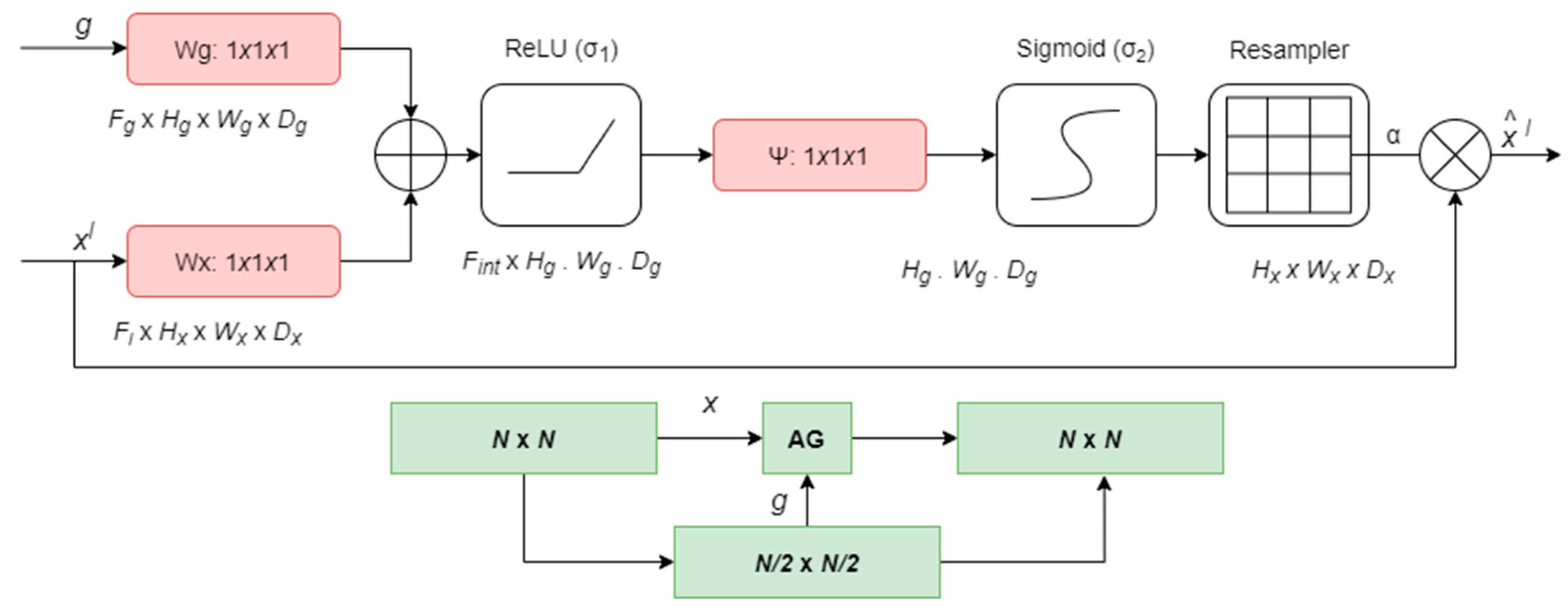
3.2. Attention U-Net

A CNN can learn hierarchical feature representations of images to perform classification tasks such as identifying landslide footprints through the low-level and high-level features of the satellite images [48]. However, to properly delineate and segment the pixels for identifying locations of landslides, especially when dealing with SAR data, more complex models are required. For this study, we modified a version of U-Net called Attn-U-Net, to classify each pixel of the image into a binary class. One of the reasons why the Attn-U-Net is well suited for this task is because it follows the classical U-Net encoder-decoder structure with skip connections, which allows the preservation of the structural integrity of the image to reduce the distortions that come with just convolution operations. Moreover, Attn-U-Nets have additional layers, such as soft attention gates [38], which allow the network to identify relevant spatial information also from low-level feature maps. The information is then propagated to the decoding phase. It is composed of two vector inputs x and g, where g comes from the lowest layer of the network (containing smaller dimensions and better feature representation), and X goes through a stridden convolution that is later summed up leading to an increase in the size of the aligned weights. The attention gates are implemented on the skip connections that actively suppress activations in irrelevant regions, thus reducing the number of redundant features. A scheme of the attention gates is visible in Figure 4.

3.3. Supervised Pixel-Based Classification

In the context of pixel-based classification and employing deep learning models like Attn-U-Nets, we utilized the concept of semantic segmentation, briefly described as a common computer vision task in which masking out regions of interest [49]. Semantic segmentation illustrates the association of pixels to class labels, in this case, landslides and non-landslides. With the help of Attn-U-Nets, we used an encoder-decoder network structure that allows the classification of each pixel into their expected prediction classes and obtaining the final output image with the same size as the input. Thus, an input image of size 64 × 64 pixels would be output as 64 × 64 using such network architectures and thus allow pixel-by-pixel manner segmentation of the image. We select this image size as the best since neither increasing it to 128 × 128 nor decreasing it to 32 × 32 increased the accuracy of the models. As training labels are important, it is also crucial to maintain a balance between the landslide and non-landslide classes. Otherwise, there can be instances of increased false negatives (actual landslides being missed out). Therefore, employing techniques like data augmentation can be very helpful in this context. However, labels could be in areas with no useful landslide-significant SAR amplitude information, therefore augmentations, here, could also be detrimental, since they could increase the number of geometrically distorted pixels in the dataset. We discuss this more in-depth in the discussion section. Nonetheless, we chose vertical and horizontal random flip augmenters considering that flipping a satellite landslide image results in newer landslide images exhibiting different landslide orientations without generating significant distortion.

The entire process was written in Python, with GIS processing handled by ArcMap and machine learning handled by TensorFlow [50]. We used Dice Loss [51] as the loss function for training the deep learning model:

$$\mathrm{Dice}\mathrm{Loss}={\displaystyle \sum }_{\mathrm{c}}1-\frac{{\sum }_{\mathrm{i}=1}^{\mathrm{N}}{\mathrm{p}}_{\mathrm{ic}}{\mathrm{g}}_{\mathrm{ic}}+\in }{{\sum }_{\mathrm{i}=1}^{\mathrm{N}}{\mathrm{p}}_{\mathrm{ic}}+{\mathrm{g}}_{\mathrm{ic}}+\in }$$

(1)

Equation (1) represents a 2-class Dice score coefficient (DSC) variation for class c, where ${\mathrm{g}}_{\mathrm{ic}}\in$ [0, 1] and ${\mathrm{p}}_{\mathrm{ic}}\in$ [0, 1] represent the ground truth and predicted labels, respectively. Furthermore, to avoid division by zero, the $\in$ ensures numerical stability, while N denotes the total number of image pixels. We employed a stochastic gradient descent approach based on an adaptive estimate of first- and second-order moments (Adam) as the loss function optimizer, which is useful in tasks in which data are noisy and/or present sparse gradients [52]. Lastly, training such deep learning models requires the right combinations of hyper-parameters to optimize the model to achieve the best possible results. Therefore, we trained the model with a series of hyper-parameter combinations iteratively, namely, the number of filters (2, 4, 8, 16, 32) and batch size (2, 4, 8, 16, 32).

3.4. Accuracy Assessment

Standard accuracy metrics Precision, Recall, F1-score, and Intersection Over-Union (IOU) were derived for the results using true positives (TP), true negatives (TN), false positives (FP), and false negatives (FN). The fraction of landslide pixels accurately recognized by the model was shown by precision (2) [53]. Recall (3) is the proportion of landslides in the labeled data that are accurately detected by the model [26], and the F1-score (4) is the balance between the Precision and the Recall metrics. The Intersection over Union (IoU) (5) approaches towards the overlap between the predictions and the ground truth.

$$\mathrm{Precision}:\mathrm{p}=\frac{\mathrm{TP}}{\left(\mathrm{TP}+\mathrm{FP}\right)}$$

(2)

$$\mathrm{Recall}:\mathrm{r}=\frac{\mathrm{TP}}{\left(\mathrm{TP}+\mathrm{FN}\right)}$$

(3)

$$\mathrm{F}1-\mathrm{score}:\mathrm{f}=2\frac{\left(\mathrm{p}·\mathrm{r}\right)}{\left(\mathrm{p}+\mathrm{r}\right)}$$

(4)

$$\mathrm{IoU}:\mathrm{i}=\frac{\mathrm{TP}}{\left(\mathrm{TP}+\mathrm{FP}+\mathrm{FN}\right)}$$

(5)

4. Results

In this section, we show the results on the employment of the Attn-U-Net model for detecting landslides on SAR imagery. Other versions of U-Net were considered in the research, such as the classical U-Net structure as well as a U-Net version with three dropout layers. To be clearer and more concise we decided to show here just the results of the Attn-U-Net configuration, which achieved the highest performances. We apply the model on two different band combinations per two Sentinel-1 orbits and evaluate the effect of augmentations for all the combinations. For each combination, hyperparameters are tuned to achieve the best possible results. As described earlier, the research aims to investigate and analyze the possibility of performing a landslide mapping task, just with SAR data and topographical factors, to set the bases for an automated all-time all-weather landslide mapping method.

Landslide Automated Mapping

The models calibrated on composites based on images from the Sentinel-1 ascending path always achieve the highest performances (see

Table 4. Performances and best hyperparameters for Attn-U-Net and BA_S datasets, with and without augmentations.

Name	Augmentations	Batch Size	Learning Rate	Filters First Layer	Precision (%)	Recall (%)	F1-Score (%)	IoU (%)
D_BA_S 1	Horizontal and Vertical flip	4	0.001	32	42.79	60.96	50.17	33.52
	None	4	0.001	32	44.66	66.53	53.37	36.43
A_BA_S 2	Horizontal and Vertical flip	16	0.001	32	55.21	66.26	60.02	42.93
	None	4	0.001	32	57.16	62.86	59.68	42.58

¹ Descending orbit: VV amplitude pre-event, VV amplitude post-event, Slope angle. ² Ascending orbit: VV amplitude pre-event, VV amplitude post-event, Slope angle.

and

Table 5. Performances and best hyperparameters for Attn-U-Net and BAA_S datasets, with and without augmentations.

Name	Augmentations	Batch Size	Learning Rate	Filters First Layer	Precision (%)	Recall (%)	F1-Score (%)	IoU (%)
D_BAA_S 1	Horizontal and Vertical flip	16	0.001	32	49.63	59.09	53.77	36.95
	None	8	0.001	32	48.43	64.23	55.15	38.13
A_BAA_S 2	Horizontal and Vertical flip	8	0.001	32	53.59	71.60	61.15	44.13
	None	8	0.001	32	53.07	66.33	58.91	42.00

¹ Descending orbit: VV amplitude pre-event, VV amplitude post-event, VV amplitude post-event, Slope angle. ² Ascending orbit: VV amplitude pre-event, VV amplitude post-event, VV amplitude post-event, Slope angle.

). As shown in Table 5, the augmented A_BAA_S dataset, achieved the best overall metrics, with the higher recall (71.60%), F1-score (61.15), and IoU score (44.13%). The higher precision is achieved by the A_BA_S without augmentations, with a value of 57.16%. In all the cases, the best learning rate is 0.001 and the optimal number of filters for the first layer is always 32. As visible in Table 4 and Table 5, the best batch size changes almost randomly, with a slight tendency to increase accordingly to the number of training samples. Therefore, a tendency to prefer bigger batch sizes after applying augmentations is noticeable. For all the datasets, the recall is higher than the precision. The worst performances are displayed by both the D_BA_S datasets and by the augmented D_BAA_S. Qualitatively, Figure 5a–c depicts the best predictions result in relation to the manually digitized landslides. This strategy is able to identify most of all of the landslides. However, some small landslides are missed and some non-landslide areas are categorized as landslides. The vegetation changes that occurred between the two SAR collections might have resulted in considerable alterations to the ground surface. As a result, further effort must be made to reduce the uncertainty induced by vegetation changes. The model spent around 7 mins carrying out predictions on the entire study area. All studies were carried out on a Mac-OS machine equipped with a 2.2 GHz Intel Core i7 processor with 6 cores, a 256-GB SSD, and 16 GB of RAM.

5. Discussion

Results show the potential of SAR amplitude data employed in combination with an advanced version of U-Net to detect landslides in the presence of cloud cover.

Prediction scores in Table 4 and Table 5 illustrate how, for the study area, the acquisition geometry of the ascending orbit can acquire more landslide-related information than the descending. Moreover, when using two backscatter acquisitions after the event (BAA_S datasets), we notice an increase in recall and a decrease in precision. Considering the ascending orbit, while the F1-score of the A_BAA_S is 1.13% higher than the A_BA_S, the latter shows higher precision, with a difference of 1.62%. Thus, more landslide pixels are correctly classified with the A_BAA_S since this composite map, being composed by three Sentinel-1 acquisitions carries more landslide-related information than the A_BA_S (two Sentinel-1 acquisitions). At the same time, the increase of false positives is related to minor changes in the background when considering a longer period, which are then wrongly classified as landslides by the model. However, with time as a key factor in rapidly mapping landslides in emergency scenarios, the employment of the BA_S dataset structure would be preferable since it requires just one post-event backscatter acquisition. In fact, for the study case, the first Sentinel-1 SAR image available for the ascending orbit was acquired just seven days after the event (13 September 2018), while the second was acquired 19 days after the event (25 September 2018).

The differences in the performance of ascending and descending orbits with and without augmentations on the training data are worthy of note. As cited above, the lower metrics are generally related to the descending path, and for this orbit, they always decrease after applying augmentations. On the other hand, when dealing with ascending orbit data, the model performance benefits when training data are augmented. This peculiar behavior is due to the intrinsic characteristics of the SAR backscatter data, which is known for presenting distorted pixels due to the interaction between the acquisition geometry and the topography [35]. Thus, by assuming equality in terms of physical soil properties, the main reason for different results between ascending and descending is due to the orientation of the slopes, which, in the specific case study, favors the ascending orbit acquisition geometry. In the study area, the descending path seems to carry less landslide-related information for the study case. Thus, when using augmentations, we enhance the number of inconsistent data, leading the model towards worse performances [54].

From a qualitative evaluation of the predictions, we can confirm a tendency of the models to overpredict the landslide class, while very few landslides are completely missed (see Figure 5). Moreover, it is noticeable how false positives are all localized around true landslides objects, and rarely scattered far from them. The explanation for this phenomenon could be found again in the peculiar characteristics of the SAR data, which may present distortions in correspondence of the actual landslides due to the landslide scars and slope geometries. Lastly, as stated above, the inventory is shaped through manual interpretation of 3 m resolution optical PlanetScope imagery. Therefore, differences both in terms of sensors and image resolution surely slightly influence the final mapping performances and validation of the models.

Furthermore, recently Aimaiti et al. [55] carried out an interesting analysis by employing pre-and post-event backscatter intensity Advanced Land Observation Satellite 2 Phased Array L-band Synthetic Aperture Radar 2 (ALOS-2 PALSAR-2) images acquired from both descending and ascending orbits. Although the data’s different resolutions and sensor wavelengths might have a significant impact on the results, false positives in correspondence of vegetation changes are found in both investigations and successfully minimized by adding slope angle. However, our research shows that training a model using data from the less suitable Sentinel-1 orbit (in this case Descending) might confuse the model by providing inconsistent data. In this scenario, combining the predictions of both orbits yields worse results than utilizing only the best-fitting orbit results (in this case Ascending). Moreover, a comparison with the results obtained by Nava et al. [39] is interesting, where the best performances were yielded by the tri-temporal SAR composite BAA (VV pre-event; VV post-event; VV post-event) and the bi-temporal plus slope composite BAS (VV pre-event; VV post-event; Slope angle) datasets. Consistency with the results of this study is discovered since the BAA S composite is nothing more than a ‘fusion’ of those two composites, resulting in a tri-temporal plus slope composite.

6. Conclusions

This study analyzed and discussed various Sentinel-1 SAR amplitude combinations and orbits to investigate and propose a rapid cross-cloud landslide detection approach. Our experiments provide encouraging results and prove the combination of Deep Learning and Sentinel-1 SAR amplitude data as a reliable method to map landslides in any weather conditions. The quantitative comparison findings revealed that the ascending intensity-based landslide predictions had the highest accuracy, for this specific case study. Not all features of the landscape were assessed due to the intricacy of forested mountain terrain and the side-looking nature of SAR sensors. Therefore, results are not as accurate as those obtainable by an optical-based DL model. Moreover, because SAR exhibits numerous distortions owing to acquisition geometry in high slope locations, which are the most prone to landslide occurrence, the approach may exhibit limits due to specific topographic characteristics of the research area. However, SAR data have the considerable advantage of collecting information regarding landslides when optical imagery is not usable or not available because of cloud cover or during night hours. Moreover, almost all the targets are detected from the automated mapping of the entire Hokkaido area, although with some shape imprecisions. In the study area, the first cloud-free Sentinel-2 image was available more than a month after the multiple landslide event, excluding the possibility of an optical-based rapid automated mapping. This study shows the possibility of performing a reliable landslide emergency rapid mapping within seven days after the event, independently from the presence of cloud cover. Thus, the approach may have relevant benefits in emergency management and civil protection operations by decreasing the time delay for the emergency response by improving the quality and frequency of hazard mapping and risk assessments.

Nevertheless, various improvements can be achieved, this being the first research proposing a DL-based segmentation approach for landslide mapping on SAR data with the help of slope as a topographical factor. For instance, numerous SAR sensors and derivates still need to be investigated, as well as the impact of different wavelengths in different environments. Moreover, in the existing literature, investigations on the combination of phase, intensity, and coherence data with DL-based approaches are still lacking. Thus, although SAR data potential is manifest, the effectiveness of such combination for landslide mapping purposes is still unknown.

References

1. Hong, H.; Chen, W.; Xu, C.; Youssef, A.M.; Pradhan, B.; Tien Bui, D. Rainfall-Induced Landslide Susceptibility Assessment at the Chongren Area (China) Using Frequency Ratio, Certainty Factor, and Index of Entropy. Geocarto Int. 2017, 32, 139–154. [Google Scholar] [CrossRef]
2. Serey, A.; Piñero-Feliciangeli, L.; Sepúlveda, S.A.; Poblete, F.; Petley, D.N.; Murphy, W. Landslides Induced by the 2010 Chile Megathrust Earthquake: A Comprehensive Inventory and Correlations with Geological and Seismic Factors. Landslides 2019, 16, 1153–1165. [Google Scholar] [CrossRef]
3. Song, K.; Wang, F.; Dai, Z.; Iio, A.; Osaka, O.; Sakata, S. Geological Characteristics of Landslides Triggered by the 2016 Kumamoto Earthquake in Mt. Aso Volcano, Japan. Bull. Eng. Geol. Environ. 2019, 78, 167–176. [Google Scholar] [CrossRef]
4. Chunga, K.; Livio, F.A.; Martillo, C.; Lara-Saavedra, H.; Ferrario, M.F.; Zevallos, I.; Michetti, A.M. Landslides Triggered by the 2016 Mw 7.8 Pedernales, Ecuador Earthquake: Correlations with ESI-07 Intensity, Lithology, Slope and PGA-h. Geosciences 2019, 9, 371. [Google Scholar] [CrossRef] [Green Version]
5. Ferrario, M.F. Landslides Triggered by Multiple Earthquakes: Insights from the 2018 Lombok (Indonesia) Events. Nat. Hazards 2019, 98, 575–592. [Google Scholar] [CrossRef]
6. Wang, F.; Fan, X.; Yunus, A.P.; Subramanian, S.S.; Alonso-Rodriguez, A.; Dai, L.; Xu, Q.; Huang, R. Coseismic Landslides Triggered by the 2018 Hokkaido, Japan (Mw 6.6), Earthquake: Spatial Distribution, Controlling Factors, and Possible Failure Mechanism. Landslides 2019, 16, 1551–1566. [Google Scholar] [CrossRef]
7. Aleotti, P.; Chowdhury, R. Landslide Hazard Assessment: Summary Review and New Perspectives. Bull. Eng. Geol. Environ. 1999, 58, 21–44. [Google Scholar] [CrossRef]
8. Quesada-Román, A.; Fallas-López, B.; Hernández-Espinoza, K.; Stoffel, M.; Ballesteros-Cánovas, J.A. Relationships between Earthquakes, Hurricanes, and Landslides in Costa Rica. Landslides 2019, 16, 1539–1550. [Google Scholar] [CrossRef]
9. Galli, M.; Ardizzone, F.; Cardinali, M.; Guzzetti, F.; Reichenbach, P. Comparing Landslide Inventory Maps. Geomorphology 2008, 94, 268–289. [Google Scholar] [CrossRef]
10. Wieczorek, G.F. Preparing a Detailed Landslide-Inventory Map for Hazard Evaluation and Reduction. Bull. Assoc. Eng. Geol. 1984, 21, 337–342. [Google Scholar] [CrossRef]
11. Reichenbach, P.; Rossi, M.; Malamud, B.D.; Mihir, M.; Guzzetti, F. A Review of Statistically-Based Landslide Susceptibility Models. Earth Sci. Rev. 2018, 180, 60–91. [Google Scholar] [CrossRef]
12. Catani, F.; Lagomarsino, D.; Segoni, S.; Tofani, V. Landslide Susceptibility Estimation by Random Forests Technique: Sensitivity and Scaling Issues. Nat. Hazards Earth Syst. Sci. 2013, 13, 2815–2831. [Google Scholar] [CrossRef] [Green Version]
13. Catani, F.; Tofani, V.; Lagomarsino, D. Spatial Patterns of Landslide Dimension: A Tool for Magnitude Mapping. Geomorphology 2016, 273, 361–373. [Google Scholar] [CrossRef] [Green Version]
14. Manconi, A.; Casu, F.; Ardizzone, F.; Bonano, M.; Cardinali, M.; de Luca, C.; Gueguen, E.; Marchesini, I.; Parise, M.; Vennari, C.; et al. Brief Communication: Rapid Mapping of Landslide Events: The 3 December 2013 Montescaglioso Landslide, Italy. Nat. Hazards Earth Syst. Sci. 2014, 14, 1835–1841. [Google Scholar] [CrossRef] [Green Version]
15. Meena; Tavakkoli Piralilou Comparison of Earthquake-Triggered Landslide Inventories: A Case Study of the 2015 Gorkha Earthquake, Nepal. Geosciences 2019, 9, 437. [CrossRef] [Green Version]
16. Mezaal, M.; Pradhan, B.; Rizeei, H. Improving Landslide Detection from Airborne Laser Scanning Data Using Optimized Dempster–Shafer. Remote Sens. 2018, 10, 1029. [Google Scholar] [CrossRef] [Green Version]
17. Blaschke, T. Object Based Image Analysis for Remote Sensing. ISPRS J. Photogramm. Remote Sens. 2010, 65, 2–16. [Google Scholar] [CrossRef] [Green Version]
18. Duro, D.C.; Franklin, S.E.; Dubé, M.G. A Comparison of Pixel-Based and Object-Based Image Analysis with Selected Machine Learning Algorithms for the Classification of Agricultural Landscapes Using SPOT-5 HRG Imagery. Remote Sens. Environ. 2012, 118, 259–272. [Google Scholar] [CrossRef]
19. Zhu, X.X.; Tuia, D.; Mou, L.; Xia, G.-S.; Zhang, L.; Xu, F.; Fraundorfer, F. Deep Learning in Remote Sensing: A Comprehensive Review and List of Resources. IEEE Geosci. Remote Sens. Mag. 2017, 5, 8–36. [Google Scholar] [CrossRef] [Green Version]
20. Chen, Z.; Zhang, Y.; Ouyang, C.; Zhang, F.; Ma, J. Automated Landslides Detection for Mountain Cities Using Multi-Temporal Remote Sensing Imagery. Sensors 2018, 18, 821. [Google Scholar] [CrossRef] [Green Version]
21. Ghorbanzadeh, O.; Blaschke, T.; Gholamnia, K.; Meena, S.R.; Tiede, D.; Aryal, J. Evaluation of Different Machine Learning Methods and Deep-Learning Convolutional Neural Networks for Landslide Detection. Remote Sens. 2019, 11, 196. [Google Scholar] [CrossRef] [Green Version]
22. Catani, F. Landslide Detection by Deep Learning of Non-Nadiral and Crowdsourced Optical Images. Landslides 2021, 18, 1025–1044. [Google Scholar] [CrossRef]
23. Meena, S.R.; Ghorbanzadeh, O.; van Westen, C.J.; Nachappa, T.G.; Blaschke, T.; Singh, R.P.; Sarkar, R. Rapid Mapping of Landslides in the Western Ghats (India) Triggered by 2018 Extreme Monsoon Rainfall Using a Deep Learning Approach. Landslides 2021, 18, 1937–1950. [Google Scholar] [CrossRef]
24. Sameen, M.I.; Pradhan, B. Landslide Detection Using Residual Networks and the Fusion of Spectral and Topographic Information. IEEE Access 2019, 7, 114363–114373. [Google Scholar] [CrossRef]
25. Ghorbanzadeh, O.; Meena, S.R.; Shahabi Sorman Abadi, H.; Tavakkoli Piralilou, S.; Zhiyong, L.; Blaschke, T. Landslide Mapping Using Two Main Deep-Learning Convolution Neural Network Streams Combined by the Dempster–Shafer Model. IEEE J. Sel. Top. Appl. Earth Obs. Remote Sens. 2021, 14, 452–463. [Google Scholar] [CrossRef]
26. Liu, P.; Wei, Y.; Wang, Q.; Chen, Y.; Xie, J. Research on Post-Earthquake Landslide Extraction Algorithm Based on Improved U-Net Model. Remote Sens. 2020, 12, 894. [Google Scholar] [CrossRef] [Green Version]
27. Prakash, N.; Manconi, A.; Loew, S. A New Strategy to Map Landslides with a Generalized Convolutional Neural Network. Sci. Rep. 2021, 11, 9722. [Google Scholar] [CrossRef]
28. Voigt, S.; Kemper, T.; Riedlinger, T.; Kiefl, R.; Scholte, K.; Mehl, H. Satellite Image Analysis for Disaster and Crisis-Management Support. IEEE Trans. Geosci. Remote Sens. 2007, 45, 1520–1528. [Google Scholar] [CrossRef]
29. Wilson, A.M.; Jetz, W. Remotely Sensed High-Resolution Global Cloud Dynamics for Predicting Ecosystem and Biodiversity Distributions. PLoS Biol. 2016, 14, e1002415. [Google Scholar] [CrossRef]
30. Williams, J.G.; Rosser, N.J.; Kincey, M.E.; Benjamin, J.; Oven, K.J.; Densmore, A.L.; Milledge, D.G.; Robinson, T.R.; Jordan, C.A.; Dijkstra, T.A. Satellite-Based Emergency Mapping Using Optical Imagery: Experience and Reflections from the 2015 Nepal Earthquakes. Nat. Hazards Earth Syst. Sci. 2018, 18, 185–205. [Google Scholar] [CrossRef] [Green Version]
31. Raspini, F.; Ciampalini, A.; del Conte, S.; Lombardi, L.; Nocentini, M.; Gigli, G.; Ferretti, A.; Casagli, N. Exploitation of Amplitude and Phase of Satellite SAR Images for Landslide Mapping: The Case of Montescaglioso (South Italy). Remote Sens. 2015, 7, 14576–14596. [Google Scholar] [CrossRef] [Green Version]
32. Tessari, G.; Floris, M.; Pasquali, P. Phase and Amplitude Analyses of SAR Data for Landslide Detection and Monitoring in Non-Urban Areas Located in the North-Eastern Italian Pre-Alps. Environ. Earth Sci. 2017, 76, 85. [Google Scholar] [CrossRef]
33. Ge, P.; Gokon, H.; Meguro, K.; Koshimura, S. Study on the Intensity and Coherence Information of High-Resolution ALOS-2 SAR Images for Rapid Massive Landslide Mapping at a Pixel Level. Remote Sens. 2019, 11, 2808. [Google Scholar] [CrossRef] [Green Version]
34. Plank, S.; Twele, A.; Martinis, S. Landslide Mapping in Vegetated Areas Using Change Detection Based on Optical and Polarimetric SAR Data. Remote Sens. 2016, 8, 307. [Google Scholar] [CrossRef] [Green Version]
35. Mondini, A.C.; Santangelo, M.; Rocchetti, M.; Rossetto, E.; Manconi, A.; Monserrat, O. Sentinel-1 SAR Amplitude Imagery for Rapid Landslide Detection. Remote Sens. 2019, 11, 760. [Google Scholar] [CrossRef] [Green Version]
36. Mondini, A. Measures of Spatial Autocorrelation Changes in Multitemporal SAR Images for Event Landslides Detection. Remote Sens. 2017, 9, 554. [Google Scholar] [CrossRef] [Green Version]
37. Mondini, A.C.; Guzzetti, F.; Chang, K.T.; Monserrat, O.; Martha, T.R.; Manconi, A. Landslide Failures Detection and Mapping Using Synthetic Aperture Radar: Past, Present and Future. Earth-Sci. Rev. 2021, 216, 103574. [Google Scholar] [CrossRef]
38. Abraham, N.; Khan, N.M. A Novel Focal Tversky Loss Function With Improved Attention U-Net for Lesion Segmentation. In Proceedings of the 2019 IEEE 16th International Symposium on Biomedical Imaging (ISBI 2019), Venice, Italy, 8–11 April 2019; pp. 683–687. [Google Scholar]
39. Nava, L.; Monserrat, O.; Catani, F. Improving Landslide Detection on SAR Data through Deep Learning. IEEE Geosci. Remote Sens. Lett. 2021, 19, 1–5. [Google Scholar] [CrossRef]
40. Matsuno, K.; Ishida, M. Geological Map of Hayakita in Scale of 50,000; Geological Survey of Japan: Tokio, Japan, 1960.
41. Osanai, N.; Yamada, T.; Hayashi, S.I.; Kastura, S.; Furuichi, T.; Yanai, S.; Murakami, Y.; Miyazaki, T.; Tanioka, Y.; Takiguchi, S.; et al. Characteristics of Landslides Caused by the 2018 Hokkaido Eastern Iburi Earthquake. Landslides 2019, 16, 1517–1528. [Google Scholar] [CrossRef]
42. Zhao, B.; Wang, Y.; Feng, Q.; Guo, F.; Zhao, X.; Ji, F.; Liu, J.; Ming, W. Preliminary Analysis of Some Characteristics of Coseismic Landslides Induced by the Hokkaido Iburi-Tobu Earthquake (5 September 2018), Japan. CATENA 2020, 189, 104502. [Google Scholar] [CrossRef]
43. Geospatial Information Authority of Japan. The 2018 Hokkaido Eastern Iburi Earthquake: Fault Model (Preliminary). Available online: https://www.gsi.go.jp/cais/topic180912-index-e.html (accessed on 17 February 2021).
44. Yamagishi, H.; Yamazaki, F. Landslides by the 2018 Hokkaido Iburi-Tobu Earthquake on September 6. Landslides 2018, 15, 2521–2524. [Google Scholar] [CrossRef] [Green Version]
45. ESA Copernicus Open Access Hub. Available online: https://scihub.copernicus.eu/dhus/#/home (accessed on 14 October 2020).
46. ESA Level-1 GRD Products. Available online: https://sentinel.esa.int/web/sentinel/technical-guides/sentinel-1-sar/products-algorithms/level-1-algorithms/ground-range-detected (accessed on 12 February 2021).
47. USGS Earth Explorer. Available online: https://earthexplorer.usgs.gov/ (accessed on 18 February 2021).
48. Marcelino, P. Transfer Learning from Pre-Trained Models. Towards Data Sci. 2018, 10, 23. [Google Scholar]
49. Pan, Z.; Xu, J.; Guo, Y.; Hu, Y.; Wang, G. Deep Learning Segmentation and Classification for Urban Village Using a Worldview Satellite Image Based on U-Net. Remote Sens. 2020, 12, 1574. [Google Scholar] [CrossRef]
50. Marcham, F. TensorFlow: Large-Scale Machine Learning on Heterogeneous Distributed Systems (Preliminary White Paper, November 9, 2015). arXiv 2016, arXiv:1603.04467. [Google Scholar]
51. Milletari, F.; Navab, N.; Ahmadi, S.-A. V-Net: Fully Convolutional Neural Networks for Volumetric Medical Image Segmentation. In Proceedings of the 2016 Fourth International Conference on 3D Vision (3DV), Stanford, CA, USA, 25–28 October 2016. [Google Scholar]
52. Kingma, D.P.; Ba, J.L. Adam: A Method for Stochastic Optimization. In Proceedings of the 3rd International Conference on Learning Representations (ICLR 2015—Conference Track Proceedings), San Diego, CA, USA, 5–8 May 2015. [Google Scholar]
53. Lormand, C.; Zellmer, G.F.; Németh, K.; Kilgour, G.; Mead, S.; Palmer, A.S.; Sakamoto, N.; Yurimoto, H.; Moebis, A. Weka Trainable Segmentation Plugin in ImageJ: A Semi-Automatic Tool Applied to Crystal Size Distributions of Microlites in Volcanic Rocks. Microsc. Microanal. 2018, 24, 667–675. [Google Scholar] [CrossRef] [PubMed]
54. Ntoutsi, E.; Fafalios, P.; Gadiraju, U.; Iosifidis, V.; Nejdl, W.; Vidal, M.; Ruggieri, S.; Turini, F.; Papadopoulos, S.; Krasanakis, E.; et al. Bias in Data-driven Artificial Intelligence Systems—An Introductory Survey. WIREs Data Min. Knowl. Discov. 2020, 10, e1356. [Google Scholar] [CrossRef] [Green Version]
55. Aimaiti, Y.; Liu, W.; Yamazaki, F.; Maruyama, Y. Earthquake-Induced Landslide Mapping for the 2018 Hokkaido Eastern Iburi Earthquake Using PALSAR-2 Data. Remote Sens. 2019, 11, 2351. [Google Scholar] [CrossRef] [Green Version]
Figure 1. Geographic location of the study area in Hokkaido, Japan, and landslides identified by Wang et al. [6].
Remotesensing 14 01449 g001
Figure 2. Data employed to create the composite images BAA_S and BA_S. (a) VV amplitude pre-event, (b) first VV amplitude post-event, (c) second VV amplitude post-event, and (d) slope angle.
Remotesensing 14 01449 g002
Figure 3. Manual landslide inventory visualized on (a) Sentinel-2 optical image and (b) D_BAA_S composite image.
Remotesensing 14 01449 g003
Figure 4. Scheme of the attention gates used in the model.
Remotesensing 14 01449 g004
Figure 5. Mapping performances in the study area on the A_BAA_S dataset, where (a) shows the true negative, true positive, false negative, and false positive predictions of the landslides produced by the model for the study area; (b) shows the landslides detected by the model versus the manual inventory for a zoomed area; and (c) shows the true negative, true positive, false negative, and false positive predictions of the landslides produced by the model for a zoomed area.
Remotesensing 14 01449 g005