Mapping Heat-Health Vulnerability Based on Remote Sensing: A Case Study in Karachi

Abstract

As a result of global climate change, the frequency and intensity of heat waves have increased significantly. According to the World Meteorological Organization (WMO), extreme temperatures in southwestern Pakistan have exceeded 54 °C in successive years. The identification and assessment of heat-health vulnerability (HHV) are important for controlling heat-related diseases and mortality. At present, heat waves have many definitions. To better describe the heat wave mortality risk, we redefine the heat wave by regarding the most frequent temperature (MFT) as the minimum temperature threshold for HHV for the first time. In addition, different indicators that serve as relevant evaluation factors of exposure, sensitivity and adaptability are selected to conduct a kilometre-level HHV assessment. The hesitant analytic hierarchy process (H-AHP) method is used to evaluate each index weight. Finally, we incorporate the weights into the data layers to establish the final HHV assessment model. The vulnerability in the study area is divided into five levels, high, middle-high, medium, middle-low and low, with proportions of 3.06%, 46.55%, 41.85%, 8.53% and 0%, respectively. Health facilities and urbanization were found to provide advantages for vulnerability reduction. Our study improved the resolution to describe the spatial heterogeneity of HHV, which provided a reference for more detailed model construction. It can help local government formulate more targeted control measures to reduce morbidity and mortality during heat waves.

1. Introduction

There is consensus among the global scientific community that climate change is increasing the frequency of extreme weather events [1]. Among the various extreme weather events, a heat wave may not be visually spectacular, but it will not only increase energy consumption but also (perhaps most concerning of all) exact direct effects on human health [2,3,4,5,6]. Generally, heat waves are described as a period of prolonged abnormally hot weather generally with or without high humidity. Due to several individual variations (e.g., age, socioeconomic status and education level) and thermal environment differences (e.g., urban heat island, vegetation and open space), the adaptation to heat waves varies markedly among distinct populations originating in various locations [7,8,9,10]. Thus, no unified standard has been established to define and grade heat waves.

While the definition of vulnerability has remained inconsistent, it cannot be separated from the demographic, environmental and social [7,11,12]. From the IPCC reports [13,14], the vulnerability was expressed as a function of three components, including exposure, sensitivity and adaptability, which has been widely accepted and applied [15,16]. Vulnerability measures the potential damage to a system when exposed to a hazard [17]. In epidemiological studies of heat mortality, some subgroups were defined as “vulnerable” for their sensitivity to external perturbation [18], for example, people older than 65, low-income earners, single person households, people below high school education, etc. [19,20,21]. Many HHV studies were developed given these subgroups data availability. Moreover, the necessity of the capacity to climate change emergencies was highlighted in the fourth and fifth IPCC meetings [1,14]. In addition to these, HHV cannot ignore the effects of the extreme climate events, which is named as exposure. Exposure can be written as a function of its intensity, frequency, and probability for any disasters [22]. While the current studies have identified heat waves as multi-featured events (e.g., the intensity, duration and frequency) [23], intensity often showed up as a single feature to represent the heat-wave hazard when land surface temperature (LST) intervene [24,25,26,27]. There is no doubt that a high correlation can be observed between the air temperature and LST [28,29,30,31]. However, few HHV studies have considered their gap in portraying human temperature perceptions in the past.

An absolute definition of a heat wave was the requirement to exceed a certain predetermined fixed temperature threshold for several continuous days [32]. Until now, various thresholds have been employed for heat-wave criterion, such as the 90th percent air temperature, the 95th percent air temperature, some fixed temperature (for example, 30 °C, 35 °C) [33,34,35,36]. Humans are born with the adaptation to temperature fluctuation, but this adaptation usually varies with geography and climate. To better understand the relationship between health and temperature, the minimum mortality temperature (MMT) was generally used to link temperature to death [37] or taken as a reference to evaluate the relative mortality risk during a heat wave [38]. The pity is that the statistics of heat-related mortality were not common for the backward countries. In other words, MMT was not available globally. Adjusting the heat-wave definition threshold to give an exact description of human body amenity is what we still need to explore.

Beyond the definition of heat wave, the selection of an appropriate quantitative evaluation method was also central to the assessment of HHV. There are various methods available at this stage. For example, the map overlay method [39], with the superiority in data processing and spatial analysis, has become the most common method. However, ignoring the variations in each layer has resulted in its loss of accuracy and reliability. In contrast, subjective weighting methods have more advantages in weight determination based on the decision makers. The analytic hierarchy process (AHP) [40], which combines qualitative and quantitative scoring by inviting experts to score, is the most popular subjective weighting method. Its drawback is the subjectivity of expert scoring and the error from hesitation. Out of subjective methodological shortcomings, scholars have proposed the objective weighting method, in which principal component analysis (PCA) [12,41] was often used for risk assessment. However, this method requires the input data follow the assumption of a normal distribution with a strong correlation. That is, although this method eliminated subjective errors and made a clear contribution of each indicator, its accuracy was overly dependent on index selection, making it unsuitable for our study. To solve the above issues, Zhu [42] developed the concept of the hesitant analytic hierarchy process (H-AHP) based on the traditional AHP. This indicator weighted method described the hesitation preferences with probabilities to erase the error caused by decision-makers and improve its performance.

South Asia, home to nearly one-fifth of the world’s population, has become one of the regions with a high risk of heat-related deaths due to the frequent occurrence of heat waves [10,43]. Actually, heat-related deaths are largely preventable as long as the spatial distribution of high-risk areas within the city is grasped in advance. The characterization of human health risks during extreme hot weather by measuring vulnerability can be helpful for formulating reasonable measures and taking immediate actions for high-risk areas, such as setting up public health interventions, monitoring and warning of heat-wave alerts, opening cooling centers, etc. and also for long-term urban planning purposes, such as modifying the urban built environment, greenfield development, etc., which can potentially remove heat-related mortality and morbidity [44,45]. Vulnerability assessment is the most widespread and popular form of the unitless measurement, describing the resilience of the population to natural disasters and hazards [46,47]. Currently, the research on heat-health vulnerability assessment (HHV) has been widely conducted in developed countries with constantly improving spatial accuracy [33,48,49,50,51,52]. However, it should be noted that the research on the spatial distribution of HHV in developing countries is still in its infancy. Existing studies have mainly been implemented at the administrative unit level, while few attempts focus on the specialized vulnerability assessment at the high-resolution raster level [53].

Therefore, this article aimed to take Karachi, Pakistan as an example to demonstrate a simple and flexible assessment framework for developing countries where demographic information and socioeconomic data are inconvenient to access. This framework relied on remote sensing data with 1 km × 1 km spatial resolution and some digital data to be easily replicated in other pivotal cities. Additionally, we introduced a concept from Yin et al. [54], named the most frequent temperature (MFT), to redefine a heat wave on accurate representation of the human body’s temperature perception, and employed the H-AHP method to the weight calculations. We hope that this research can inform a reference for a more precise HHV assessment model in the future.

2. Materials and Methods

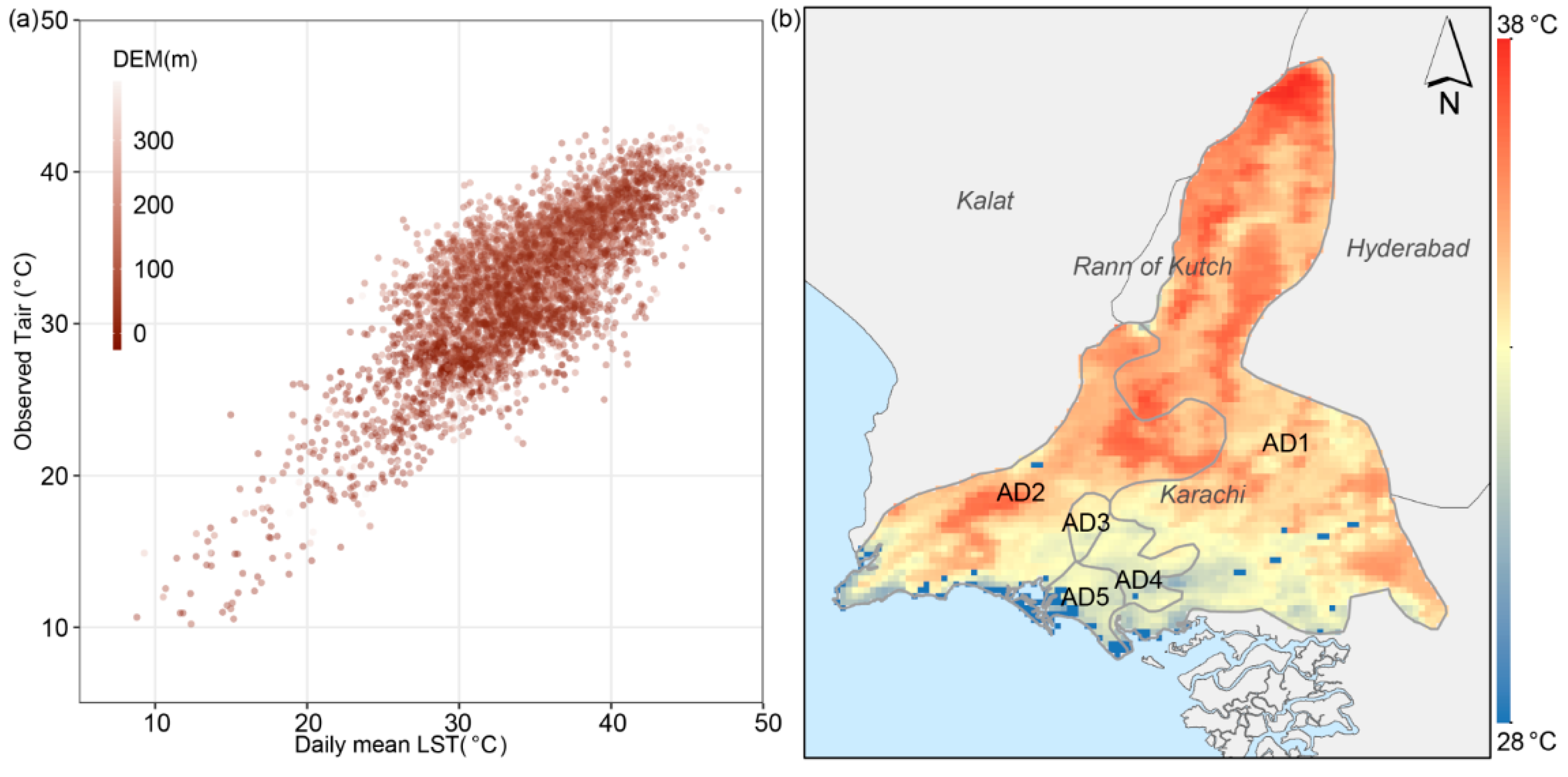
2.1. Data Sources

To provide a visual representation of the data used in this study, we list all the relevant information including their name, source, spatial resolution, temporal resolution and description in

Table 1. Descriptions of the datasets.

Name	Spatial Resolution	Temporal Resolution	Source	Description
MOD11A1/MYD11A1	1 km × 1 km	Daily	https://ladsweb.modaps.eosdis.nasa.gov/search/, accessed on 20 June 2019	MODIS/Terra, Aqua Land Surface Temperature data. The basic data used to determine the intensity of heat waves (C1).
MOD13A3	1 km × 1 km	Monthly	https://ladsweb.modaps.eosdis.nasa.gov/search/, accessed on 20 June 2019	MODIS/Terra vegetation indices data, describing vegetation coverage (C6).
MOD02KM	1 km × 1 km	Daily	https://ladsweb.modaps.eosdis.nasa.gov/search/, accessed on 20 June 2019	Level 1B calibrated radiances, which are used to calculate the NDBI to describe the coverage of impermeable surfaces (C3).
DMSP/OLS	1 km × 1 km	Year	https://www.ngdc.noaa.gov/eog/dmsp/, accessed on 20 June 2019	DMSP-OLS night light data, which reflect the level of regional development and measure the urbanization level (C8).
GDP	1 km × 1 km	Year	[55]	GDP (C7) reflects the ability of a county to finance itself in a disaster-response process.
Age and sex Structure	100 m × 100 m	Year	https://www.worldpop.org/geodata/, accessed on 20 June 2019	These data describe the distribution of vulnerable people (C4) over 65 years old.
Poverty	1 km × 1 km	Year	https://www.worldpop.org/geodata/, accessed on 20 June 2019	Proportion of residents living in MPI-defined poverty (C2).
Pakistan POI	-	Year	https://www.openstreetmap.org/, accessed on 1 May 2019	We mainly use the data to confirm the location of hospitals and calculate the distance from medical resources (C5).
Meteorological Station Data	-	Daily	https://www.ncei.noaa.gov/maps/hourly/, accessed on 10 July 2021	The observation data of meteorological stations, which are used to count the occurrence of heat waves.

. The observation meteorological data here had two main uses: We used a total of 28 stations, located within Pakistan, to capture the relationship between LST and near surface air temperature (T_air). In addition, the only station in Karachi was used to monitor the annual variation of the T_air and record the heat wave duration. For Moderate Resolution Imaging Spectroradiometer (MODIS) LST, there were 120 (30 days × 4 images per day) LST images used for T_air estimation, in which four images per day were pooled into the daily LST via averaging. In addition, we selected the day with the maximum mean daily temperature during the longest heat-wave duration (26 June 2016 in this study) to represent the intensity of heat wave with the reference of observation data. The missing data resulting from cloud cover were filled by the mean value within three neighboring days. The age and sex structure data were collected with the spatial resolution of 100 m × 100 m and were resampled to 1 km × 1 km by count summation. The points of interest within Pakistan (Pakistan POIs) were employed for the calculation of the Euclidean distance from medical resources. More detailed of all data properties were available via the link given on the source.

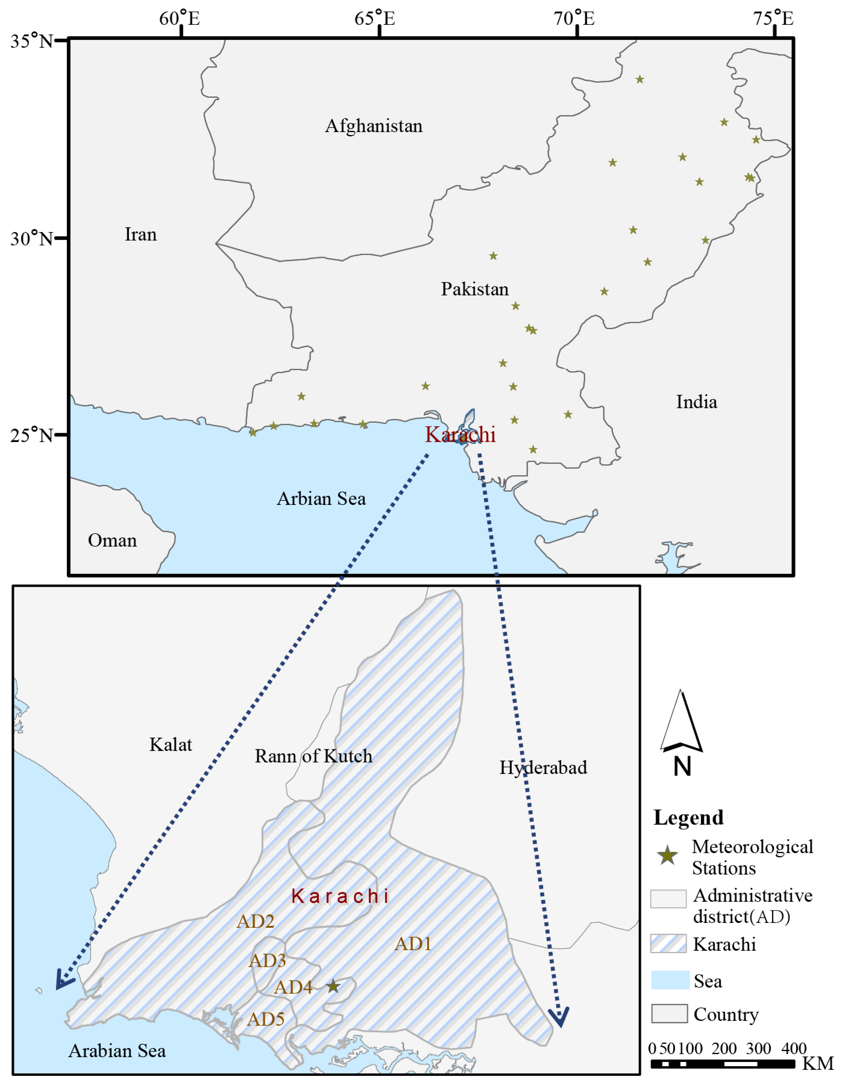
2.2. Overview of the Study Area

Karachi, as the largest city in Pakistan, is located on the southern coast of Pakistan, northwest of the Indus Delta, south of the Arabian Sea, and on the plain between the Julie River and Mariel River (as shown in Figure 1). This city has a population of approximately 20 million people and covers an area of 3527 km², of which the urban area covers 1821 km². This area experiences a tropical climate encompassing warm winters and hot summers [56]. The average minimum temperature in winter is 13 °C, and the average maximum temperature in summer is 34 °C. Rainfall is scarce, with an average annual precipitation of only 200 mm.

Since the 1990s, Pakistan’s economy has been slow with a per capita income of approximately $600. In Sindh Province, where Karachi is located, over half of the population lives below the poverty line. Some areas have poverty rates over 80%. The metropolitan attraction and cultural diversity have led to an influx of migration into Karachi. In this case, a drastic population expansion has appeared in this region. Currently, the city is under tremendous pressure for jobs, housing, transportation and supplies of water and electricity, increasing the heat wave risk. Moreover, this city is crowded with a large number of residents of the Islamic faith. Ramadan customs also increase the mortality risk from heat waves. That is to say, assessing the heat wave risk level in Karachi and clarifying its spatial variations are quite paramount for rational planning of infrastructure construction and reduction in morbidity.

2.3. Methods and Procedure

We identified and assessed the HHV in the study area based on the following steps: first, specify the time of heat wave occurrence; then, assessment indicators selection and HHV assessment model construction; next, index weight calculation; and finally, results accuracy evaluation.

2.3.1. Heat Wave Definition

One common feature in the association between temperature and mortality is MMT, which is defined as the temperature where the minimum mortality rate is reached. It is a fixed temperature for variable geographic and subgroups with poor availability in undeveloped areas for its expensive cost at collection. Compared to MMT, MFT, the daily mean temperature occurs most frequently within a year, is a plain variable. Yin et al. [54] revealed a high consistency and stability between the MMT and the MFT in the same area during the same period by exploring the temperature-death relationship in 420 cities. In a word, using the MFT as a surrogate for the MMT, the mean error is only 0.9 °C (95% Confidence interval (CI): 0–3 °C). This finding provided a new idea for defining heat wave. Based on the existing criteria, we classified days with daily mean temperatures higher than the MFT of the region as hot days. When hot days lasted for more than 3 days, this period was called a heat wave. Under this concept, we use the daily mean temperature instead of the maximum temperature considering the mean temperature has been proven to be a better predictor of mortality than maximum and minimum temperatures as it is more likely to represent the temperature level across 24 h [57]. Heat-related mortality is widely known to be more severe when the temperature remains high within 24 h, causing inability of the body to cool down [58].

2.3.2. Determination of the Vulnerability Assessment Factors

Exposure

Temperature is traditionally captured from meteorological stations. The spatial interpolation method [59,60,61,62,63,64,65,66,67] can generate continuous surfaces from meteorological observation data with higher temporal resolution, but its accuracy is always affected by their sparse distribution and is sensitive to the season [60]. Compared with it, the moderate resolution imaging spectroradiometer land surface temperature (MODIS LST) can better describe the spatial heterogeneity of the temperature and has a good correlation with the air temperature (T_air) observation [61,62], even though there still have some gaps in the temporal resolution that need to be filled.

Here, we chose the mean MODIS LST (mean LST of four satellite transit times per day) as the basic data for exposure assessment because of the sparsity of meteorological stations in the study area (there are only two available stations). To describe the heat mortality exposure of heat waves as clearly as possible, we screened out the day with the maximum temperature during the longest heat wave. For this study, we chose 26 June 2016, when the mean temperature reached 34.6 °C and the maximum temperature reached 40 °C. We estimated the daily mean T_air from daily mean MODIS LST using linear regression. The selected meteorological stations (as shown in Figure 1) are all in Pakistan, for which the elevation is less than 500 m. Data from 1 April 2016 to 31 September 2016 were all used to estimate the coefficients for its seasonal similarity. Then, exposure results were used for the final assessment. Estimating the air temperature from the LST is a common and relatively simple algebraic method, and the relationship between the two was also affected by the variation of the land cover, weather and elevation [68,69], which we did not consider at this time. Since we have removed the impact of other variables as possible by selecting the similar stations.

$${\mathrm{T}}_{\mathrm{air}}=\mathrm{a}\times \mathrm{LST}+\mathrm{b}$$

(1)

where T_air(C1) is the estimated T_air and a and b are coefficients calculated from the selected stations.

Sensitivity

Several individual subgroups, such as elderly individuals over the age of 65 [70,71,72] and those living in the poverty [73] have been indicated to have greater sensitivity over the past decade. Apart from the above subgroups, urban areas may be more sensitive to heat than surrounding rural areas [74]. For city dwellers, the urban heat island (UHI) effect will cause additional risks because heat waves have shown more potential to amplify UHIs [75,76]. However, the UHI intensity is inequitably distributed in cities, where people of lower socioeconomic status typically live in areas with less vegetation and more heat-absorbing surfaces [7,8,9]. The main factor causing the UHI is the city’s underlying surface, which is often dominated by buildings [77]. Therefore, we used an impermeable surface ratio here to indicate the city dwellers who will be more troubled by the UHI. On this basis, the poverty rate (C2) and the vulnerable population (elderly individuals over 65 years old) (C4) were also selected as the main index factors in the sensitivity assessment layer. Here, we chose the normalized difference built-up index (NDBI) [78] (C3) to represent the distribution of impervious areas.

Adaptability

With the development of technology in recent years, the resolution of night-time light data has been continuously improved. Defense Meteorological Satellite Program Operational Line Scanner (DMSP/OLS) night-time light data (C8) have become an effective means for estimating the level of urbanization, population density, electric energy consumption and other factors [79,80]. A region’s adaptability to disaster mainly depends on the local medical excellence and financial status. Urban residents have access to more high-quality education, healthcare, housing, transportation and financial resources than people living in underdeveloped zones [81,82], meaning a stronger capacity to cope with the disasters. In this article, the GDP (C7) was selected to indicate the national economic development and government expenditure. The distance from a medical institution (C5) was selected to indicate the timeliness of obtaining professional medical rescue services. Furthermore, green coverage (C6) was selected to indicate the cooling effect for the surrounding area [83].

Above all, four indicators, namely, the urbanization level, green coverage, distance from a medical institution and GDP, were selected as the main index factors for adaptability assessment. Here, the euclidean distance was used to calculate the distance from a medical institution. The normalized difference vegetation index (NDVI) [84] is used to calculate the green coverage in a region of interest (ROI). As a note, all the above data used in vulnerability assessment were dimensionless with a resample value from 0 to 1 under maximum-minimum method.

2.3.3. Quantification of Evaluation Factors Based on H-AHP

Determining the weights of different evaluation indices is the key to model construction. The traditional AHP [85] can decompose complex analytical problems into different factors, but the greatest flaw of this method is that the hesitation process and uncertainty of the decision-makers during their judgment cannot be completely eliminated. To solve this problem, this paper choose the H-AHP method proposed by Zhu et al. [86] to calculate the weight in order to prevent this sort of problem. The specific steps are as follows:

• The decision-making problem is decomposed into several structural levels from top to bottom, which can be divided into target and rule layers and index levels. In this paper, it has been divided into exposure B1, sensitivity B2 and adaptability B3. Three experts in related fields (UHI remote sensing monitoring, geomorphology and natural disaster assessment, night light remote sensing and heat wave risk assessment) were invited to make important judgments this time. The specific hierarchical structure is shown in

  Table 2. Hierarchy of heat health vulnerability assessment and the weight of each indicator. The field, named Description, shows the impact of each index on HHV as positive (aggravate the vulnerability of heat-related morbidity/mortality) or negative (reduce the vulnerability of heat-related morbidity/mortality).

  Target Layer	Rule Layer	Index Layer	Weight W	Description
  Vulnreability A	Exposure B1	Intensity C1	1.00	Positive
  	Sensitivity B2	Poverty Rate C2	0.18	Positive
  		Impervious Surface C3	0.13	Positive
  		Vulnerable Population C4	0.68	Positive
  	Adaptability B3	Proximity to Medical Institutions C5	0.58	Negative
  		Green Coverage C6	0.15	Negative
  		GDP C7	0.17	Negative
  		Urbanization Level C8	0.10	Negative

  .
• The probabilistic hesitation product preference relation is then constructed. For set X = {X1, X2, ..., Xn}, it is assumed that the decision-maker (DM) can compare the elements in X in pairs, and then the probabilistic hesitation preference information according to the expert opinion is obtained, while the following probabilistic hesitation matrix preference relation (P-HMPR) is defined:

$$\mathrm{Y}={\left({\mathrm{y}}_{\mathrm{ij}}\right)}_{\mathrm{n}\times \mathrm{n}}$$

(2)

where ${\mathrm{y}}_{\mathrm{ij}}=\left(\mathrm{y}{\left(\mathrm{l}\right)}_{\mathrm{ij}}\left(\mathrm{p}{\left(\mathrm{l}\right)}_{\mathrm{ij}}\right){\displaystyle |}\mathrm{l}=1,\cdots \left|{\mathrm{y}}_{\mathrm{ij}}\right|{\displaystyle |}\right),\left|\mathrm{y}\right|$ is the number of possible values of y, and ${\mathrm{y}}_{\mathrm{ij}}$ is the preference of ${\mathrm{x}}_{\mathrm{i}}$ to ${\mathrm{x}}_{\mathrm{j}}$, which satisfies the following:

$${\mathrm{y}}_{\mathrm{ij}}^{\mathsf{\rho }\left(\mathrm{l}\right)}{\mathrm{y}}_{\mathrm{ji}}^{\mathsf{\rho }\left(\mathrm{l}\right)}{=1,\mathrm{y}}_{\mathrm{ij}}=1,\left|{\mathrm{y}}_{\mathrm{ij}}\right|=\left|{\mathrm{y}}_{\mathrm{ji}}\right|{,\mathrm{p}}_{\mathrm{ij}}^{\mathsf{\rho }\left(\mathrm{l}\right)}{=\mathrm{p}}_{\mathrm{ji}}^{\mathsf{\rho }\left(\mathrm{l}\right)},\mathrm{i},\mathrm{j}=1,2,\cdots ,\mathrm{n}$$

(3)

$${\mathrm{y}}_{\mathrm{ij}}^{\mathsf{\rho }\left(\mathrm{l}\right)}\le {\mathrm{y}}_{\mathrm{ij}}^{\mathsf{\rho }\left(\mathrm{l}+1\right)},\mathrm{i}<\mathrm{j}$$

(4)

where ${\mathrm{y}}_{\mathrm{ij}}^{\mathsf{\rho }\left(\mathrm{l}\right)}$ represents the $\mathsf{\rho }$ possible values of ${\mathrm{y}}_{\mathrm{ij}}$ and ${\mathrm{p}}_{\mathrm{ij}}^{\mathsf{\rho }\left(\mathrm{l}\right)}$ is the probability of ${\mathrm{y}}_{\mathrm{ij}}^{\mathsf{\rho }\left(\mathrm{l}\right)}$.

According to the HHV assessment index system constructed above, based on a 1–9 scale, relevant experts were invited to use each indicator in the index layer as the dominant element to conduct a pairwise comparison, which was subject to the given hesitation preference information. Then, a P-HMPR of each rule layer was constructed.

c.

Consistency testing ensures the validity of the preference information and the correctness of the results. In this paper, the row geometric mean method (RGMM) proposed by Crawford and Williams [87] was selected.

According to the RGMM, the priorities ${\mathrm{w}}_{\mathrm{i}}(\mathrm{i}=1,2,\dots ,\mathrm{n})$ can be simply found as the geometric means of the rows of A:

$${\mathrm{w}}_{\mathrm{i}}=\frac{{\left({\prod }_{\mathrm{j}=1}^{\mathrm{n}}{\mathrm{y}}_{\mathrm{ij}}\right)}^{\frac{1}{\mathrm{n}}}}{{\sum }_{\mathrm{i}=1}^{\mathrm{n}}{\left({\prod }_{\mathrm{j}=1}^{\mathrm{n}}{\mathrm{y}}_{\mathrm{ij}}\right)}^{\frac{1}{\mathrm{n}}}}$$

(5)

Based on Equation (5), Aguarón and Moreno-Jiménez [88] proposed the geometric consistency index (GCI) for evaluating the consistency of ${\mathrm{MPR}\mathrm{Y}}^{\left(\mathrm{l}\right)}={\left({\mathrm{y}}_{\mathrm{ij}}^{\left(\mathrm{l}\right)}\right)}_{\mathrm{n}\times \mathrm{n}}$ as follows:

$${\mathrm{GCI}}_{\mathrm{Y}\left(\mathrm{l}\right)}=\frac{2}{\left(\mathrm{n}-1\right)\left(\mathrm{n}-2\right)}{\sum }_{\mathrm{i}<\mathrm{j}}{\log }^2{\mathrm{e}}_{\mathrm{ij}}{,\mathrm{e}}_{\mathrm{ij}}=\frac{{\mathrm{y}}_{\mathrm{ij}}^{\left(\mathrm{l}\right)}{\mathrm{w}}_{\mathrm{j}}}{{\mathrm{w}}_{\mathrm{i}}}$$

(6)

Let Y be a hesitant-judgment space; then, the consistency index of the expected set of Y can be defined as:

$${\mathrm{E}\left(\mathrm{GCI}\right)}_{\mathrm{Y}}=\left({\prod }_{\mathrm{i},\mathrm{j}=1}^{\mathrm{n}}\frac{1}{\left|{\mathrm{y}}_{\mathrm{ij}}\right|}\right){\sum }_{\mathrm{Y}}{\mathrm{GCI}}_{\mathrm{Y}\left(\mathrm{l}\right)}$$

(7)

Compared with the consistency ratio, Aguarón and Moreno-Jiménez [86] proposed the thresholds of GCI for different sizes of Y. Among these equations, the calculation of $\mathrm{E}{\left(\mathrm{GCI}\right)}_{\mathrm{Y}}$ is based on Monte Carlo simulations [89], a common random sampling method used to solve problems having a probabilistic interpretation, to obtain the GCI values of the preference relations of the various probabilistic hesitation product types. If $\mathrm{E}{\left(\mathrm{GCI}\right)}_{\mathrm{Y}}\le {\mathrm{GCI}}^{\mathrm{n}}$, then Y is with the acceptable consistency; otherwise, Y is inconsistent. For the unacceptable consistency, the iterative method given by Zeshui and Cuiping [90] were chosen as a basis to develop consistency improvement. All probabilistic hesitation product preferences established in this paper passed the consistency test via MATLAB experiments.

d.

Based on the RGMM, hesitant preference analysis (HPA) was applied to determine the ranking of the weights of the corresponding elements of the same layer corresponding to the relative importance of the elements of the upper layer. For P-HMPR, a probabilistic hesitation judgment space is composed of the hesitation judgment, and the H-AHP method [53] analyses this space to obtain the priorities of objectives with HPA.

For P-HMPR ${\mathrm{Y}=(\mathrm{y}}_{\mathrm{ij}}{)}_{\mathrm{n}\times \mathrm{n}}$, where ${\mathrm{y}}_{\mathrm{ij}=}{(\mathrm{y}}_{\mathrm{ij}}^{\left(\mathrm{l}\right)}\left({\mathrm{p}}_{\mathrm{ij}}^{\left(\mathrm{l}\right)}\right)|\mathrm{l}=1,\cdots ,\left|\mathrm{y}\right|)$, a comparison matrix ${\mathrm{Y}}^{\left(\mathrm{l}\right)}{=(\mathrm{y}}_{\mathrm{ij}}^{\left(\mathrm{l}\right)}{)}_{\mathrm{n}\times \mathrm{n}}$ can be obtained from Y following the probability distributions ${\mathrm{p}}_{\mathrm{ij}}{=\mathrm{p}}_{\mathrm{ij}}^{\left(\mathrm{l}\right)}(\mathrm{l}=1,\cdots ,\left|{\mathrm{y}}_{\mathrm{ij}}\right|)$. Let ${\mathrm{f}}_{\mathrm{ij}}{(\mathrm{y}}_{\mathrm{ij}}^{\left(\mathrm{l}\right)})$ be the density function of ${\mathrm{y}}_{\mathrm{ij}}$; then, the joint probability distribution of ${\mathrm{y}}_{\mathrm{ij}}^{\left(\mathrm{l}\right)}(\mathrm{i},\mathrm{j}=1,2,\cdots ,\mathrm{n})$ is specified by a density function $\mathrm{f}({\mathrm{y}}^{\left(\mathrm{l}\right)})$ as follows:

$$\mathrm{f}({\mathrm{y}}^{\left(\mathrm{l}\right)})={\displaystyle \prod }_{\mathrm{i},\mathrm{j}=1}^{\mathrm{n}}{\mathrm{f}}_{\mathrm{ij}}\left({\mathrm{y}}^{\left(\mathrm{l}\right)}\right)$$

(8)

According to ${\mathrm{Y}}^{\left(\mathrm{l}\right)}$ and Equation (5), we can obtain a priority vector denoted by ${\mathsf{\omega }}^{\left(\mathrm{l}\right)}{=(\mathsf{\omega }}_1^{\left(\mathrm{l}\right)}{,\mathsf{\omega }}_2^{\left(\mathrm{l}\right)},\cdots {,\mathsf{\omega }}_{\mathrm{n}}^{\left(\mathrm{l}\right)})$. Then, elements can be sorted from the best rank (r = 1) to the worst rank (r = n) by the following ranking function:

$${\mathrm{rank}}_{\mathrm{i}}\left({\mathsf{\omega }}^{\left(\mathrm{l}\right)}\right)=1+{\displaystyle \sum }_{\mathrm{k}=1}^{\mathrm{n}}{\mathsf{\rho }(\mathsf{\omega }}_{\mathrm{k}}^{\left(\mathrm{l}\right)}{>\mathsf{\omega }}_{\mathrm{i}}^{\left(\mathrm{l}\right)})=\mathrm{r}$$

(9)

where $\mathsf{\rho }\left(\mathrm{true}\right)=1,\mathsf{\rho }\left(\mathrm{false}\right)=0$. Let Y be a hesitant-judgment space, and based on the ranking function, the judgments that make the objective ${\mathrm{x}}_{\mathrm{i}}$ ranking $\mathrm{r}$ in the space can be analysed as follows:

$${\mathrm{Y}}_{\mathrm{i}}^{\mathrm{r}}\left({\mathrm{y}}^{\left(\mathrm{l}\right)}\right)=\left\{{\mathrm{y}}^{\left(\mathrm{l}\right)}\in {\mathrm{Y}:\mathrm{rank}}_{\mathrm{i}}\left({\mathsf{\omega }}^{\left(\mathrm{l}\right)}\right)=\mathrm{r}\right\}$$

(10)

Based on Equations (8) and (10), the acceptability rate of ${\mathrm{x}}_{\mathrm{i}}$ ranking $\mathrm{r}$ can be defined as a rank acceptability index ${\mathrm{b}}_{\mathrm{i}}^{\mathrm{r}}$. It is computed as the expected volume of ${\mathrm{Y}}_{\mathrm{i}}^{\mathrm{r}}{(\mathrm{y}}^{\left(\mathrm{l}\right)})$:

$${\mathrm{b}}_{\mathrm{i}}^{\mathrm{r}}={\int }_{{\mathrm{Y}}_{\mathrm{i}}^{\mathrm{r}}\left({\mathrm{y}}^{\left(\mathrm{l}\right)}\right)}\mathrm{f}\left({\mathrm{y}}^{\left(\mathrm{l}\right)}\right){\mathrm{dy}}^{\left(\mathrm{l}\right)}$$

(11)

where ${\mathrm{b}}_{\mathrm{i}}^{\mathrm{r}}ϵ\left[0,1\right],{\sum }_{\mathrm{r}=1}^{\mathrm{n}}{\mathrm{b}}_{\mathrm{i}}^{\mathrm{r}}=1$. The Monte Carlo simulation process can be used to compute ${\mathrm{b}}_{\mathrm{i}}^{\mathrm{r}}$.

With respect to the ranking acceptability indices, the acceptable probabilities of the objectives for each rank can be clearly identified. The acceptable probabilities for all ranks can be aggregated as a comprehensive ranking value, which can be implemented through aggregation operators, such as ordered weighted averaging (OWA) [91].

Letting ${\mathrm{h}}_{\mathrm{i}}$ be the holistic evaluation of ${\mathrm{x}}_{\mathrm{i}}$, then it is computed as:

$${\mathrm{h}}_{\mathrm{i}}={\displaystyle \sum }_{\mathrm{r}=1}^{\mathrm{n}}{\mathrm{w}}_{\mathrm{r}}{\mathrm{b}}_{\mathrm{i}}^{\mathrm{r}}$$

(12)

Starting from the bottom layer of the structure, the indicator weights (${\mathrm{w}}_{\mathrm{r}}$) in each layer were calculated. The results are summarized in Table 2, and the specific algorithm was established using MATLAB software.

2.3.4. Establishment of the Evaluation Model Based on the Map Overlay Method

First, to eliminate the mapping interval inconsistency problem of different data, we standardized each indicator layer. It should be noted that the normalization of the negative indicators is opposite to that of the positive ones, i.e., the larger the value is, the more it tends to 0 after normalization.

Finally, Equation (7) was used to calculate the rule layer index (RLI, e.g., B1, B2, B3) and Equation (8) was used to calculate the heat health vulnerability (HHV) for this region.

$$\mathrm{RLI}={\sum }_{\mathrm{i}=1}^{\mathrm{n}}{\mathrm{w}}_{\mathrm{i}}\times {\mathrm{x}}_{\mathrm{ij}}$$

(13)

$$\mathrm{HHV}=\left(\mathrm{B}1+\mathrm{B}2+\mathrm{B}3\right)/3$$

(14)

where ${\mathrm{W}}_{\mathrm{i}}$ is the index weight obtained based on the H-AHP and ${\mathrm{x}}_{\mathrm{ij}}$ is the standardized value of the index. Finally, we mapped the HHV for the study area and divided it into five grades of high, medium-high, medium, medium-low and low according to the equal interval method.

3. Results

3.1. Heat-Wave Statistics

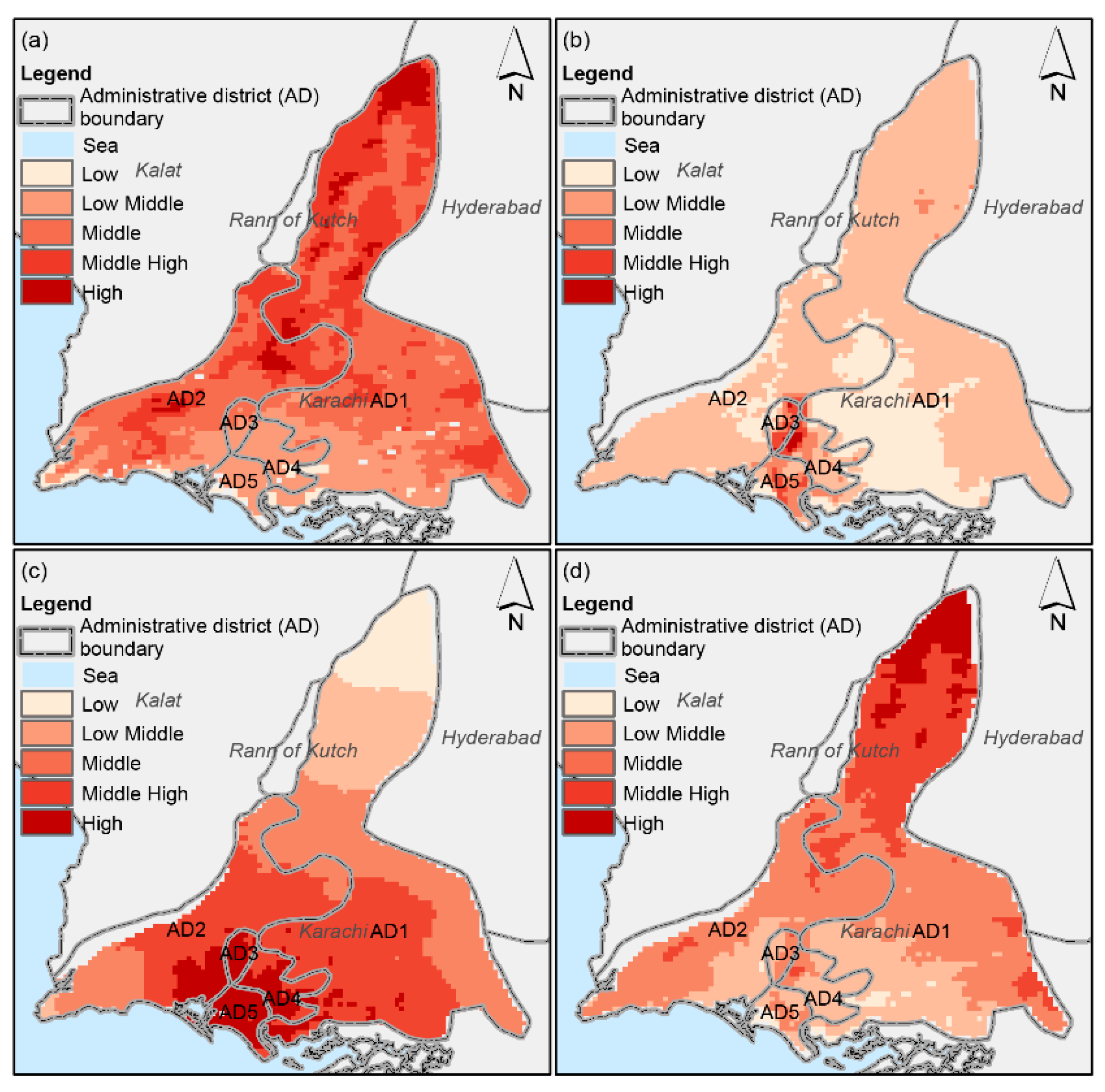
With the cloud coverage remote sensing images usually have some missing data causing the heat wave process cannot be complete observed. However, the meteorological station can significantly remedy this defect. Here, we use observed data to clarify the frequency and intensity of heat waves in 2016 in Karachi based on our definition. The only meteorological station, named JINNAH INTERNATIONAL, is located in the northeast of Karachi (geographical coordinates: 24.907, 67.161) with an altitude of 30.5 m. As statistics, the MFT in this region was 30 °C in 2016 (all data were rounded up before the statistics on its frequency), which occurred 57 times throughout this year. The results indicated 91 hot days in Karachi during 2016, with 6 times heat waves. Among these, the longest duration was 59 days, lasting from 8 May to 6 July. The annual daily mean temperature variation in 2016 was shown in Figure 2.

3.2. Exposure

For estimating daily mean T_air from daily mean LST, a and b were calculated as 0.71 and 8.06, respectively. Figure 3a showed a high correlation between the daily mean LST and the observed daily mean T_air, whose R-square (R²) was 0.63. Based on the estimated T_air, the area where T_air was higher than the local MFT (30 °C) accounted for over 97% on 26 June 2016, and the maximum temperature exceeded 37 °C. Areas where T_air reached above 35 °C were mainly concentrated in Malir and Karachi west with scattered distribution in the other regions.

Figure 4a showed the exposure distribution of Karachi. The proportions of each grade (low, medium-low, medium, medium-high and high) were 2.38%, 20.92%, 41.94%, 27.46%, and 4.77%, respectively. The low-middle to middle-high grade exhibited the widest distribution, occupying almost all of Karachi except the northern barren zone. Among all the residential areas, the suburbs located Karachi west and Malir, which were obviously separated from the main urban areas, were all located in high-exposure areas and should be vigilant.

3.3. Sensitivity

Among sensitivity assessment, we found the suburbs and southeast of the main districts gathered many poor people, such as Karachi central, Karachi south, etc. These regions were severely aging but relatively wealthy. On the basis of the equal interval method, the area proportion of each grade from low to high was as follows: 23.52%, 71.07%, 3.36%, 1.64%, and 0.42%. Karachi central and Karachi south showed high-level sensitivity, while Karachi west, Karachi east, and Malir north showed medium-high sensitivity. Other areas showed medium-low grades and even below. That is to say, Karachi central was obviously more sensitive and may become the worst-hit area during heat waves, which needs to be focused on in the future.

3.4. Adaptability

According to Figure 4c, the adaptability in the southwestern parts of Malir, Karachi Central, Karachi South, Karachi East, and the eastern of Karachi West is the most superior. The coastland has rich medical resources and ishighly urbanized. Within these districts, the green space coverage is higher in the east. but the economy is more developed in the west, bringing together industry. In contrast, several suburbs and non-city regions have limited resilience in disaster response due to scarce resources. According to the classification, the area proportion of each grade from low to high is 11.21%, 38.50%, 29.29%, 12.88% and 8.13%. Judging from its distribution, northern Karachi central, Malir cantonment, Karachi east, Korangi, Karachi west and Malir are all key areas of concern. This result also proves the indispensablility of medical institutions during disasters, which serves as a reminder to improve the allocation of health care resources during urban development planning. At the same time, grassland and shrubs cannot play a shading role and thus they have a poor cooling effect and limited contribution to prevention.

3.5. Heat-Health Vulnerability

This assessment was conducted by stacking the above three criterion layers on the basis of Equation (10). Statistically, the areas with HHV level from low to high are 99 km², 1505 km², 1353 km², 276 km², and 0 km², accounting for 3.06%, 46.55%, 41.85%, 8.53% and 0% of the total area. We found that more than 50% of the areas had middle to high vulnerability. Only the northern part of Malir shows middle-high vulnerability. Karachi central, as the city with the highest concentration of aging population, was more vulnerable (middle-high risk) than other urban areas. For the full region, the west of Karachi West and the east of Karachi East had higher vulnerability levels. However, large residential areas were not located in these regions, the morbidity and death rates caused by heat waves will not be high. Despite this, we still suggested the local government paying more attention to these areas, particularly Karachi central, and focus on strengthening infrastructure construction, attaching importance to the risk prevention and raising residents’ awareness of heat waves.

3.6. Verification

The calculation of each indicator’s weight was the key to our model. There were many studies agree on making distinctions between the contributions of different indicators [34,53,92]. However, the selection of indicators in each study is certainly not the same, and thus, is inconvenient to copy from them directly. Comparing the rank of different indicators is one way to prove the credibility of our judgment. Therefore, we summarized the weight of indicators we choose this time from similar studies (

Table 3. The weight of indicators in similar studies.

	Tran et al., 2020 [92]	Estoque et al., 2020 [38]	Hulley et al., 2019 [98]	Oh et al., 2017 [99]	Phung et al., 2016 [100]
Sensitivity
Poverty rate	0.11	0.44	0.21	-	0.09
Impervious Surface	0.09	-	-	-	-
Vulnerable Population	0.18	0.57	0.62	0.2	0.12
Adaptability
Proximity to Medical Institutions	0.31	-	-	0.58	0.14
Green Coverage	0.27	0.46	-	-	-
GDP	-	0.32	-	0.21	-
Urbanization Level	-	0.22	-	-	-

). It can be seen that the rank of each indicator conforms to our conclusion. For example, the weight ranking was as Proverty rate > vulnerability population > impervious surface in the sensitivity layer from Tran et.al [92], which was consistent with our results.

Located in a climatically warm geographical region, Pakistan is vulnerable to extreme climate events such as heat waves, droughts, and floods [91]. In the literature, many heatwave related studies have been conducted in this region from different perspectives [10,15,93,94]. Through a comparison, we verified the veracity of this study. The results from ThinkHzard [95] show that Karachi, which is located in southern Pakistan, is a high heat hazard area. In their study, they used the wet bulb globe temperature (WBGT, in °C), which has a notable relevance to human health, to describe the heat-wave hazard. However, their conclusion is basically consistent with ours. Except this, the heat-related mortality risk prediction studies in Pakistan can also give some certain references. These studies, which rely on various models [94,96,97], all showed a similar conclusion with ours, i.e., the heat-related mortality risk (the same as our HHV) ranges from middle to high. As shown in Figure 4, the HHV area with a higher than middle risk level reached over 50%. In comparison, our mapping provides more details in spatial distribution, which provided a more powerful reference for the government to formulate effective preventive measures.

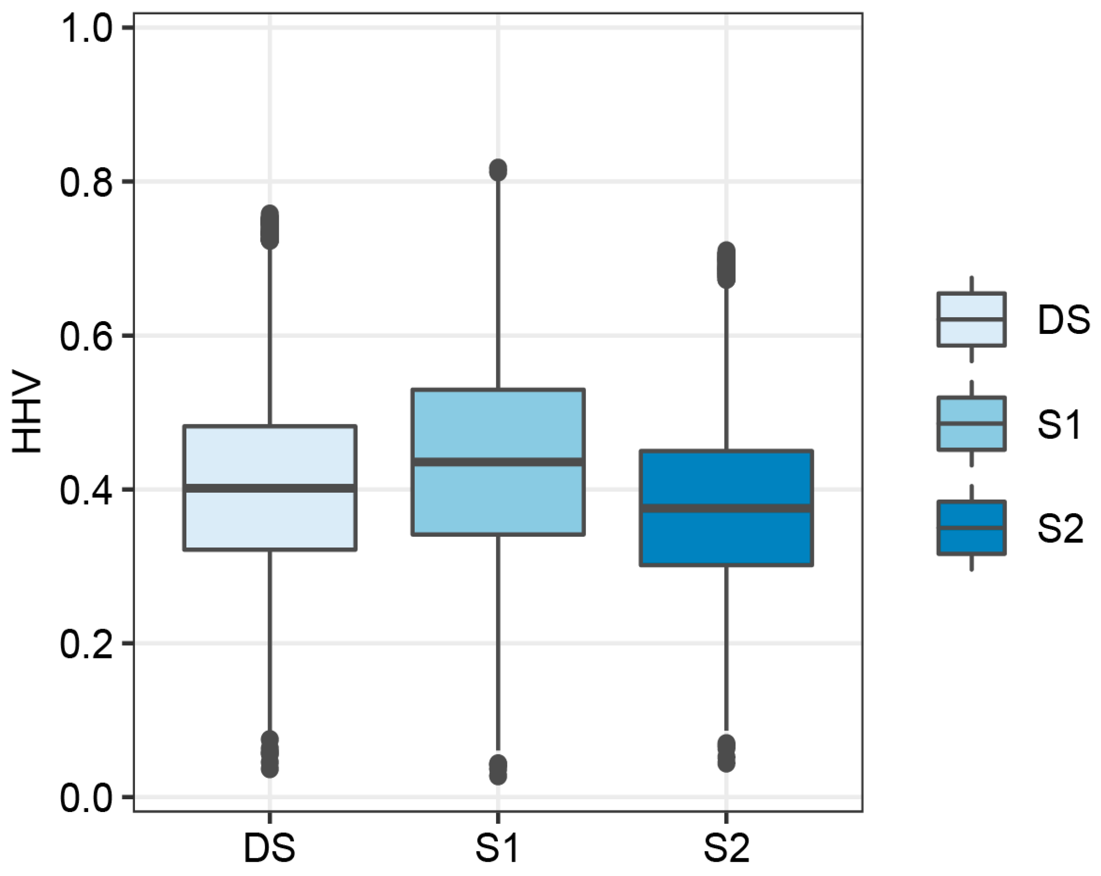
3.7. Sensitivity Analysis

We changed our settings of each rule layer weight in order to assess the robustness of our model with the designed following scenarios. Specifically, two scenarios of sensitivity analysis (S1 and S2) were set randomly without any support. In addition, we can find the unnoticed variations in the Figure 5, reminding us the potential impact of indicators weighted is not significant.

DS: the default model setting of our model with the average weighted among exposure, sensitivity and adaptability.

S1: the weight among exposure, sensitivity and adaptability are 0.5, 0.25, 0.25, respectively.

S2: the weight among exposure, sensitivity and adaptability are 0.2, 0.4, 0.4, respectively.

4. Discussion

Building a more reproducible HHV system will help understand high-vulnerability areas around the world. In this study, we established a kilometre-level HHV system with widely available data. Although the accuracy of this system can be generally verified, this model still has certain limitations.

Meteorological site and LST data [101,102,103] are the most common temperature data used in climate change research. For application, site data with poor spatial resolution often fails to meet expectations. LST data can effectively solve the problem of the uneven distribution of stations, but there are still deviations from the air temperature [104]. Here we estimated Tair from LST using a simple and common linear regressionmodel with limited precision which can be further improved. In addition, the data used to evaluate the exposure was the most severe single-day data of annual heat waves. It can describe the high-exposure distribution within the study area at the highest temperature. However, the continuous influence of heat waves was not considered, and thus, this model is more suitable for single-day assessment. How to eliminate the gaps in the satellite spatial-temporal data to achieve long-term continuous monitoring still requires more research.

Moreover, the mortality risk [105,106,107,108] has appeared in many studies. Since the heat-related mortality data was generally unavaiable for this study area, we redefine a heat wave by regarding the MFT as the minimum temperature threshold for HHV in order to illustrate the discomfort caused by extreme temperatures. This is the first known study performed in this manner, and we can do more to prove its universality through delving deeper.

Vulnerability analysis is usually divided into qualitative and quantitative procedures, of which the former will be described as high, medium or low level, while the latter will be described as a specific previously defined risk metric (e.g., the number of potential victims, economic losses, etc.) [109]. Especially when it is difficult to obtain quantitative data, qualitative analysis is more common. Earlier, the spatial vulnerability assessment models were developed based on the map overlay with equal weights, which depended on the basic multiplication, division or addition and subtraction [82,109,110]. As the complexity of the model increases, an ever-increasing number of scholars have realized that the contributions of different factors are not the same. The distinction of the index weights determines the specific performance. The combination of AHP and Geographic Information System (GIS) exists extensively within qualitative natural disaster risk assessment, such as floods, landslides and drought risks [111,112,113,114,115,116,117]. Considering that this method has a subjective influence that is difficult to eliminate, the fuzzy analytic hierarchy process (FAHP) and improved analytic hierarchy process (IAHP) methods [118,119,120] were used to reduce the subjective error. Here, we choose the H-AHP method. The main purpose is to provide a feasible HHV method reference for developing countries with limited spatial data availability. However, its applicability still requires complete and detailed demonstration. Moreover, an in-depth discussion is also needed to determine which approach is more scientific when considering the distinction between the subjective and objective weighted assignment.

The purpose of the constructed model is to determine the locations of regions with a high vulnerability and provide a reference for future proposals of rectification plans for specific defects. Considering the applicability of the model, all the data selected in this paper are publicly available, and this method is simple and easy to implement. At present, such an evaluation system cannot serve as an early warning system for heat-wave disasters. Under these circumstances, the manner in which spatial data are used to establish a heat-wave disaster early warning system to realize the implementation of disaster monitoring and vulnerability estimation is also the focus of future research in this field.

5. Conclusions

Heat waves are major climate disasters that occur throughout the world. At this stage, a unified HHV system for heat waves has not been established. The accuracies of the different evaluation methods are still being explored. Based on previous studies, this paper proposes a new method. We use the H-AHP method to calculate the weight of each evaluation index. Then, a comprehensive assessment model based on spatial data is constructed according to the weights of the different index layers, and the distribution and impact factor of the heat-wave vulnerability affecting Karachi, Pakistan, are calculated. This work has certain reference significance to better understand the vulnerability to heat waves and establish a heat-wave identification, monitoring and evaluation system.

Based on the assessment, the low-vulnerability area covered 99 km², and the middle-low vulnerability area covered 1505 km², while the total area with a middle vulnerability was 1353 km². The total area with a middle-high vulnerability was 276 km², and the high-vulnerability area totaled 0 km². The analysis revealed that a wide range of medical institutions and a high urbanization level can reduce the HHV to a certain extent, but the influence of green space coverage depends on the characteristics of the vegetation itself, such as the shading performance and the cooling effect. For Karachi, it is important to pay attention to the infrastructure in high-vulnerability areas and provide more protection for the elderly to reduce the incidence of disease and death caused by heat waves. In addition, the pervasion of indoor “cooling centres” is also a good way to avoid risks. This study was based on kilometre-level gridded spatial data. However, the limitation of the spatial data acquisition and cost, we did not consider the impacts of more sophisticated indicators such as air-conditioning ownership, which bring an inevitable error in our HHV results. It should be noticed that the HHV still have some limitation in its application. For example, it was not a universal spatial description for any years, only providing a reference for risk perception. In the future, these important indicators should be incorporated in to improve the comprehensiveness of the assessment. In addition, the spatial resolution should be further improved following the highest resolution satellite development.

References

1. IPCC. Climate Change 2014: Impacts, Adaptation, and Vulnerability. Working Group II Contribution to the Fifth Assessment Report of the Intergovernmental Panel on Climate Change; Cambridge University Press: Cambridge, UK; New York, NY, USA, 2014. [Google Scholar]
2. Robine, J.M.; Cheung, S.L.K.; Le Roy, S.; Van Oyen, H.; Griffiths, C.; Michel, J.P.; Herrmann, F.R. Death toll exceeded 70,000 in Europe during the summer of 2003. Comptes. Rendus. Biologies. 2008, 331, 171–178. [Google Scholar] [CrossRef] [PubMed]
3. Barriopedro, D.; Fischer, E.M.; Luterbacher, J.; Garcia-Herrera, R. The hot summer of 2010: Redrawing the temperature record map of Europe. Science 2011, 332, 220–224. [Google Scholar] [CrossRef] [PubMed] [Green Version]
4. Mazdiyasni, O.; AghaKouchak, A.; Davis, S.J.; Madadgar, S.; Mehran, A.; Ragno, E.; Sadegh, M.; Sengupta, A.; Ghosh, S.; Dhanya, C.T.; et al. Increasing probability of mortality during Indian heat waves. Sci. Adv. 2017, 3, e1700066. [Google Scholar] [CrossRef] [PubMed] [Green Version]
5. Fuhrmann, C.M.; Sugg, M.M.; Konrad, C.E.; Waller, A. Impact of extreme heat events on emergency department visits in North Carolina (2007–2011). J. Community Health 2016, 41, 146–156. [Google Scholar] [CrossRef]
6. Merte, S. Estimating heat wave-related mortality in Europe using singular spectrum analysis. Clim. Change 2017, 142, 321–330. [Google Scholar] [CrossRef]
7. Harlan, S.L.; Brazel, A.J.; Prashad, L.; Stefanov, W.L.; Larsen, L. Neighborhood microclimates and vulnerability to heat stress. Soc. Sci. Med. 2006, 63, 2847–2863. [Google Scholar] [CrossRef]
8. Harlan, S.L.; Declet-Barreto, J.H.; Stefanov, W.L.; Petitti, D.B. Neighborhood effects on heat deaths: Social and environmental predictors of vulnerability in Maricopa County, Arizona. Environ. Health Perspect. 2013, 121, 197–204. [Google Scholar] [CrossRef] [Green Version]
9. Declet-Barreto, J.; Knowlton, K.; Jenerette, G.D.; Buyantuev, A. Effects of urban vegetation on mitigating exposure of vulnerable populations to excessive heat in Cleveland, Ohio. Weather Clim. Soc. 2016, 8, 507–524. [Google Scholar] [CrossRef]
10. Shi, P.; Wang, J.; Xu, W.; Ye, T.; Yang, S.; Liu, L.; Fang, W.; Liu, K.; Li, N.; Wang, M. World Atlas of Natural Disaster Risk; Springer: Berlin/Heidelberg, Germany, 2015; pp. 309–323. [Google Scholar]
11. Füssel, H.M. Vulnerability: A generally applicable conceptual framework for climate change research. Glob. Environ. Change 2007, 17, 155–167. [Google Scholar] [CrossRef]
12. Johnson, D.P.; Stanforth, A.; Lulla, V.; Luber, G. Developing an applied extreme heat vulnerability index utilizing socioeconomic and environmental data. Appl. Geogr. 2012, 35, 23–31. [Google Scholar] [CrossRef]
13. IPCC. Climate Change 2001: Impacts, Adaptation, And Vulnerability: Contribution of Working Group II to the Third Assessment Report of the Intergovernmental Panel on Climate Change; Cambridge University Press: Cambridge, UK, 2001. [Google Scholar]
14. IPCC. Climate Change 2007: Impacts, Adaptation and Vulnerability. Contribution of Working Group II to the Fourth Assessment Report of the Intergovernmental Panel on Climate Change; Cambridge University Press: Cambridge, UK, 2007. [Google Scholar]
15. Malik, S.M.; Awan, H.; Khan, N. Mapping vulnerability to climate change and its repercussions on human health in Pakistan. Glob. Health 2012, 8, 31. [Google Scholar] [CrossRef] [PubMed] [Green Version]
16. De Sherbinin, A.; Bukvic, A.; Rohat, G.; Gall, M.; McCusker, B.; Preston, B.; Apotsos, A.; Fish, C.; Kienberger, S.; Muhonda, P.; et al. Climate vulnerability mapping: A systematic review and future prospects. Wiley Interdiscip. Rev. Clim. Change 2019, 10, e600. [Google Scholar] [CrossRef]
17. Turner, B.L.; Kasperson, R.E.; Matson, P.A.; McCarthy, J.J.; Corell, R.W.; Christensen, L.; Eckley, N.; Kasperson, J.X.; Luers, A.; Martello, M.L.; et al. A framework for vulnerability analysis in sustainability science. Proc. Natl. Acad. Sci. USA 2003, 100, 8074–8079. [Google Scholar] [CrossRef] [PubMed] [Green Version]
18. Stafoggia, M.; Forastiere, F.; Agostini, D.; Biggeri, A.; Bisanti, L.; Cadum, E.; Caranci, N.; de’Donato, F.; Lisio, S.D.; Maria, M.D.; et al. Vulnerability to heat-related mortality: A multicity, population-based, case-crossover analysis. Epidemiology 2006, 17, 315–323. [Google Scholar] [CrossRef]
19. Vescovi, L.; Rebetez, M.; Rong, F. Assessing public health risk due to extremely high temperature events: Climate and social parameters. Clim. Res. 2005, 30, 71–78. [Google Scholar] [CrossRef]
20. Macnee, R.G.D.; Tokai, A. Heat wave vulnerability and exposure mapping for Osaka City, Japan. Environ. Syst. Decis. 2016, 36, 368–376. [Google Scholar] [CrossRef]
21. Christenson, M.; Geiger, S.D.; Phillips, J.; Anderson, B.; Losurdo, G.; Anderson, H.A. Heat vulnerability index mapping for Milwaukee and Wisconsin. J. Public Health Manag. Pract. 2017, 23, 396–403. [Google Scholar] [CrossRef]
22. Wannous, C.; Velasquez, G. United nations office for disaster risk reduction (unisdr)—Unisdr’s contribution to science and technology for disaster risk reduction and the role of the international consortium on landslides (icl). In Proceedings of the Workshop on World Landslide Forum, Ljubljana, Slovenia, 29 May–2 June 2017; Springer: Cham, Switzerland, 2017; pp. 109–115. [Google Scholar]
23. Savić, S.; Marković, V.; Šećerov, I.; Pavić, D.; Arsenović, D.; Milošević, D.; Dolinaj, D.; Nagy, I.; Pantelić, M. Heat wave risk assessment and mapping in urban areas: Case study for a midsized Central European city, Novi Sad (Serbia). Nat. Hazards 2018, 91, 891–911. [Google Scholar] [CrossRef]
24. Ho, H.C.; Knudby, A.; Huang, W. A spatial framework to map heat health risks at multiple scales. Int. J. Environ. Res. Public Health 2015, 12, 16110–16123. [Google Scholar] [CrossRef] [Green Version]
25. Hoerling, M.; Kumar, A.; Dole, R.; Nielsen-Gammon, J.W.; Eischeid, J.; Perlwitz, J.; Quan, X.W.; Zhang, T.; Pegion, P.; Chen, M. Anatomy of an extreme event. J. Clim. 2013, 26, 2811–2832. [Google Scholar] [CrossRef]
26. Buscail, C.; Upegui, E.; Viel, J.F. Mapping heatwave health risk at the community level for public health action. Int. J. Health Geogr. 2012, 11, 38. [Google Scholar] [CrossRef] [PubMed] [Green Version]
27. Kestens, Y.; Brand, A.; Fournier, M.; Goudreau, S.; Kosatsky, T.; Maloley, M.; Smargiassi, A. Modelling the variation of land surface temperature as determinant of risk of heat-related health events. Int. J. Health Geogr. 2011, 10, 7. [Google Scholar] [CrossRef] [PubMed] [Green Version]
28. Liu, Y.; Quan, W. Research on high temperature indices of Beijing city and its spatiotemporal pattern based on satellite data. Climatic Environ. Res. 2014, 19, 332–342. [Google Scholar]
29. Flores, F.; Lillo, M. Simple air temperature estimation method from MODIS satellite images on a regional scale. Chil. J. Agric. Res. 2010, 70, 436–445. [Google Scholar] [CrossRef] [Green Version]
30. Zhang, W.; Huang, Y.; Yu, Y.; Sun, W. Empirical models for estimating daily maximum, minimum and mean air temperatures with MODIS land surface temperatures. Int. J. Remote Sens. 2011, 32, 9415–9440. [Google Scholar] [CrossRef]
31. Hou, P.; Chen, Y.; Qiao, W.; Cao, G.; Jiang, W.; Li, J. Near-surface air temperature retrieval from satellite images and influence by wetlands in urban region. Theor. Appl. Climatol. 2013, 111, 109–118. [Google Scholar] [CrossRef]
32. Robinson, P.J. On the definition of a heat wave. J. Appl. Meteorol. 2001, 40, 762–775. [Google Scholar] [CrossRef]
33. Aubrecht, C.; Özceylan, D. Identification of heat risk patterns in the US National Capital Region by integrating heat stress and related vulnerability. Environ. Int. 2013, 56, 65–77. [Google Scholar] [CrossRef]
34. Ahmadnezhad, E.; Holakouei, N.K.; Ardalan, A.; Mahmoudi, M.; Younesian, M.; Naddafi, K.; Mesdaghinia, A.R. Excess mortality during heat waves, Tehran Iran: An ecological time-series study. J. Res. Health Sci. 2013, 13, 24–31. [Google Scholar]
35. Analitis, A.; Michelozzi, P.; D’Ippoliti, D.; de’Donato, F.; Menne, B.; Matthies, F.; Atkinson, R.W.; Inigues, C.; Basagana, X.; Schneider, A.; et al. Effects of heat waves on mortality: Effect modification and confounding by air pollutants. Epidemiology 2014, 25, 15–22. [Google Scholar] [CrossRef]
36. Heo, S.; Bell, M.L.; Lee, J.T. Comparison of health risks by heat wave definition: Applicability of wet-bulb globe temperature for heat wave criteria. Environ. Res. 2019, 168, 158–170. [Google Scholar] [CrossRef] [PubMed]
37. Tomlinson, C.J.; Chapman, L.; Thornes, J.E.; Baker, C.J. Including the urban heat island in spatial heat health risk assessment strategies: A case study for Birmingham, UK. Int. J. Health Geogr. 2011, 10, 42. [Google Scholar] [CrossRef] [PubMed] [Green Version]
38. Estoque, R.C.; Ooba, M.; Seposo, X.T.; Togawa, T.; Hijioka, Y.; Takahashi, K.; Nakamura, S. Heat health risk assessment in Philippine cities using remotely sensed data and social-ecological indicators. Nat. Commun. 2020, 11, 1581. [Google Scholar] [CrossRef] [PubMed] [Green Version]
39. Xie, P.; Wang, Y.L.; Peng, J.; Liu, Y. Health related urban heat wave vulnerability assessment: Research progress and framework. Prog. Geo. 2015, 34, 165–174. [Google Scholar]
40. Aidya, O.S.; Kumar, S. Analytic hierarchy process: An overview of applications. Eur. J. Oper. Res. 2006, 169, 1–29. [Google Scholar] [CrossRef]
41. Reid, C.E.; O’neill, M.S.; Gronlund, C.J.; Brines, S.J.; Brown, D.G.; Diez-Roux, A.V.; Schwartz, J. Mapping community determinants of heat vulnerability. Environ. Health Perspect. 2009, 117, 1730–1736. [Google Scholar] [CrossRef] [PubMed]
42. Zhu, B. Decision Making Methods and Applications Based on Preference Relations; Southeast University: Nanjing, China, 2014; pp. 35–36. [Google Scholar]
43. Honda, Y.; Kondo, M.; McGregor, G.; Kim, H.; Guo, Y.L.; Hijioka, Y.; Oka, K.; Takano, S.; Hales, S.; Kovats, R.S. Heat-related mortality risk model for climate change impact projection. Environ. Health Prev. Med. 2014, 19, 56–63. [Google Scholar] [CrossRef]
44. Boumans, R.J.M.; Phillips, D.L.; Victery, W.; Fontaine, T.D. Developing a model for effects of climate change on human health and health–environment interactions: Heat stress in Austin, Texas. Urban Clim. 2014, 8, 78–99. [Google Scholar] [CrossRef]
45. (CDC) Centers for Disease Control and Prevention. Heat-Related Mortality—Arizona, 1993–2002, and United States, 1979–2002. MMWR Morb. Mortal. Wkly. Rep. 2005, 54, 628–630. [Google Scholar]
46. Flanagan, B.E.; Gregory, E.W.; Hallisey, E.J.; Heitgerd, J.L.; Lewis, B. A social vulnerability index for disaster management. J. Homel. Secur. Emerg. Manag. 2011, 8, 3. [Google Scholar] [CrossRef]
47. Conlon, K.C.; Mallen, E.; Gronlund, C.J.; Berrocal, V.J.; Larsen, L.; O’neill, M.S. Mapping human vulnerability to extreme heat: A critical assessment of heat vulnerability indices created using principal components analysis. Environ. Health Perspect. 2020, 128, 097001. [Google Scholar] [CrossRef] [PubMed]
48. Rosenthal, J.K.; Kinney, P.L.; Metzger, K.B. Intra-urban vulnerability to heat-related mortality in New York City, 1997–2006. Health Place 2014, 30, 45–60. [Google Scholar] [CrossRef] [PubMed] [Green Version]
49. Weber, S.; Sadoff, N.; Zell, E.; de Sherbinin, A. Policy-relevant indicators for mapping the vulnerability of urban populations to extreme heat events: A case study of Philadelphia. Appl. Geogr. 2015, 63, 231–243. [Google Scholar] [CrossRef]
50. Morabito, M.; Crisci, A.; Gioli, B.; Gualtieri, G.; Toscano, P.; Di Stefano, V.; Orlandini, S.; Gensini, G.F. Urban-hazard risk analysis: Mapping of heat-related risks in the elderly in major Italian cities. PLoS ONE 2015, 10, e0127277. [Google Scholar] [CrossRef] [PubMed] [Green Version]
51. Papathoma-Koehle, M.; Promper, C.; Bojariu, R.; Cica, R.; Sik, A.; Perge, K.; Laszlo, P.; Czikora, E.B.; Dumitrescu, A.; Turcus, C.; et al. A common methodology for risk assessment and mapping for south-east Europe: An application for heat wave risk in Romania. Nat. Hazards 2016, 82, 89–109. [Google Scholar] [CrossRef] [Green Version]
52. Jedlovec, G.; Crane, D.; Quattrochi, D. Urban heat wave hazard and risk assessment. Results Phys. 2017, 7, 4294–4295. [Google Scholar] [CrossRef]
53. Zhu, Q.; Liu, T.; Lin, H.; Xiao, J.; Luo, Y.; Zeng, W.; Wei, Y.; Chu, C.; Baum, S.; Du, Y.; et al. The spatial distribution of health vulnerability to heat waves in Guangdong Province, China. Glob. Health Action 2014, 7, 25051. [Google Scholar] [CrossRef] [Green Version]
54. Yin, Q.; Wang, J.; Ren, Z.; Li, J.; Guo, Y. Mapping the increased minimum mortality temperatures in the context of global climate change. Nat. Commun. 2019, 10, 4640. [Google Scholar] [CrossRef] [Green Version]
55. Kummu, M.; Taka, M.; Guillaume, J.H. Gridded global datasets for gross domestic product and Human Development Index over 1990–2015. Sci. Data 2018, 5, 1–15. [Google Scholar] [CrossRef] [Green Version]
56. Wikipedia. Climate of Karachi. February 2019. Available online: https://en.wikipedia.org/wiki/Climate_of_Karachi (accessed on 10 July 2021).
57. Chen, K.; Bi, J.; Chen, J.; Chen, X.; Huang, L.; Zhou, L. Influence of heat wave definitions to the added effect of heat waves on daily mortality in Nanjing, China. Sci. Total Environ. 2015, 506, 18–25. [Google Scholar] [CrossRef]
58. Bobb, J.F.; Peng, R.D.; Bell, M.L.; Dominici, F. Heat-related mortality and adaptation to heat in the United States. Environ. Health Perspect. 2014, 122, 811–816. [Google Scholar] [CrossRef] [PubMed]
59. Holdaway, M.R. Spatial modeling and interpolation of monthly temperature using kriging. Clim. Res. 1996, 6, 215–225. [Google Scholar] [CrossRef] [Green Version]
60. Dodson, R.; Marks, D. Daily air temperature interpolated at high spatial resolution over a large mountainous region. Clim. Res. 1997, 8, 1–20. [Google Scholar] [CrossRef]
61. Kurtzman, D.; Kadmon, R. Mapping of temperature variables in Israel: Sa comparison of different interpolation methods. Clim. Res. 1999, 13, 33–43. [Google Scholar] [CrossRef] [Green Version]
62. Carrera-Hernández, J.J.; Gaskin, S.J. Spatio temporal analysis of daily precipitation and temperature in the Basin of Mexico. J. Hydrol. 2007, 336, 231–249. [Google Scholar] [CrossRef]
63. Hengl, T.; Heuvelink, G.; Perčec Tadić, M.; Pebesma, E.J. Spatio-temporal prediction of daily temperatures using time-series of MODIS LST images. Theor. Appl. Climatol. 2012, 107, 265–277. [Google Scholar] [CrossRef] [Green Version]
64. Stewart, S.B.; Nitschke, C.R. Improving temperature interpolation using MODIS LST and local topography: A comparison of methods in south east Australia. Int. J. Climatol. 2017, 37, 3098–3110. [Google Scholar] [CrossRef]
65. Wu, T.; Li, Y. Spatial interpolation of temperature in the United States using residual kriging. Appl. Geogr. 2013, 44, 112–120. [Google Scholar] [CrossRef]
66. Oyler, J.W.; Dobrowski, S.Z.; Holden, Z.A.; Running, S.W. Remotely sensed land skin temperature as a spatial predictor of air temperature across the conterminous United States. J. Appl. Meteorol. Climatol. 2016, 55, 1441–1457. [Google Scholar] [CrossRef]
67. Zhou, Y.; Zhu, S.; Hua, J.; Li, Y.; Xiang, J.; Ding, W. Spatio-temporal distribution of high temperature heat wave in Nanjing. J. Geogr. Inf. Sci. 2018, 20, 1613–1621. [Google Scholar]
68. Gallo, K.; Hale, R.; Tarpley, D.; Yu, Y. Evaluation of the relationship between air and land surface temperature under clear-and cloudy-sky conditions. J. Appl. Meteorol. Climatol. 2011, 50, 767–775. [Google Scholar] [CrossRef]
69. Good, E.J.; Ghent, D.J.; Bulgin, C.E.; Remedios, J.J. A spatiotemporal analysis of the relationship between near-surface air temperature and satellite land surface temperatures using 17 years of data from the ATSR series. J. Geophys. Res. Atmos. 2017, 122, 9185–9210. [Google Scholar] [CrossRef]
70. Rey, G.; Fouillet, A.; Bessemoulin, P.; Frayssinet, P.; Dufour, A.; Jougla, E.; Hémon, D. Heat exposure and socio-economic vulnerability as synergistic factors in heat-wave-related mortality. Eur. J. Epidemiol. 2009, 24, 495–502. [Google Scholar] [CrossRef] [PubMed]
71. Chen, K.; Zhou, L.; Chen, X.; Ma, Z.; Liu, Y.; Huang, L.; Bi, J.; Kinney, P.L. Urbanization level and vulnerability to heat-related mortality in Jiangsu Province, China. Environ. Health Perspect. 2016, 124, 1863–1869. [Google Scholar] [CrossRef]
72. Xu, Z.; Etzel, R.A.; Su, H.; Huang, C.; Guo, Y.; Tong, S. Impact of ambient temperature on children’s health: A systematic review. Environ. Res. 2012, 117, 120–131. [Google Scholar] [CrossRef] [Green Version]
73. Madrigano, J.; Ito, K.; Johnson, S.; Kinney, P.L.; Matte, T. A case-only study of vulnerability to heat wave–related mortality in New York City (2000–2011). Environ. Health Perspect. 2015, 123, 672–678. [Google Scholar] [CrossRef]
74. Zhao, L.; Lee, X.; Smith, R.B.; Oleson, K. Strong contributions of local background climate to urban heat islands. Nature 2014, 511, 216–219. [Google Scholar] [CrossRef]
75. Wilhelmi, O.V.; Purvis, K.L.; Harriss, R.C. Designing a geospatial information infrastructure for mitigation of heat wave hazards in urban areas. Nat. Hazards Rev. 2004, 5, 147–158. [Google Scholar] [CrossRef] [Green Version]
76. Ramamurthy, P.; Bou-Zeid, E. Heatwaves and urban heat islands: A comparative analysis of multiple cities. J. Geophys. Res. Atmos. 2017, 122, 168–178. [Google Scholar] [CrossRef]
77. Ji, C.P. Impact of urban growth on the heat island in Beijing. Chin. J. Geophys. 2006, 49, 69–77. [Google Scholar]
78. Zha, Y.; Ni, S.; Yang, S. An effective approach to automatically extract urban land-use from TM imagery. J. Remote Sens. 2003, 7, 37–40. [Google Scholar]
79. Takashima, M.; Hayashi, H.; Kimura, H.; Kohiyama, M. Earthquake damaged area estimation using DMSP/OLS night-time imagery-application for Hanshin-Awaji earthquake. In Proceedings of the IEEE 2000 International Geoscience and Remote Sensing Symposium (IGARSS 2000)—Taking the Pulse of the Planet: The Role of Remote Sensing in Managing the Environment, Honolulu, HI, USA, 24–28 July 2000; IEEE: Piscataway, NJ, USA, 2000; Volume 1, pp. 336–338. [Google Scholar]
80. Chand, T.R.K.; Badarinath, K.V.S.; Elvidge, C.D.; Tuttle, B.T. Spatial characterization of electrical power consumption patterns over India using temporal DMSP-OLS nighttime satellite data. Int. J. Remote Sens. 2009, 30, 647–661. [Google Scholar] [CrossRef]
81. Bulkeley, H.; Tuts, R. Understanding urban vulnerability, adaptation and resilience in the context of climate change. Local Environ. 2013, 18, 646–662. [Google Scholar] [CrossRef] [Green Version]
82. Wilhelmi, O.V.; Hayden, M.H. Connecting people and place: A new framework for reducing urban vulnerability to extreme heat. Environ. Res. Lett. 2010, 5, 014021. [Google Scholar] [CrossRef]
83. Yu, Z.; Xu, S.; Zhang, Y.; Jørgensen, G.; Vejre, H. Strong contributions of local background climate to the cooling effect of urban green vegetation. Sci. Rep. 2018, 8, 6798. [Google Scholar] [CrossRef]
84. Burgan, R.E. Monitoring Vegetation Greenness with Satellite Data; US Department of Agriculture, Forest Service, Intermountain Research Station: Fort Collins, CO, USA, 1993. [Google Scholar]
85. Saaty, T.L. A scaling method for priorities in hierarchical structures. J. Math. Psychol. 1977, 15, 234–281. [Google Scholar] [CrossRef]
86. Zhu, B.; Xu, Z.; Zhang, R.; Hong, M. Hesitant analytic hierarchy process. Eur. J. Oper. Res. 2016, 250, 602–614. [Google Scholar] [CrossRef]
87. Crawford, G.; Williams, C. A note on the analysis of subjective judgment matrices. J. Math. Psychol. 1985, 29, 387–405. [Google Scholar] [CrossRef]
88. Aguarón, J.; Moreno-Jiménez, J.M. The geometric consistency index: Approximated thresholds. Eur. J. Oper. Res. 2003, 147, 137–145. [Google Scholar] [CrossRef]
89. Zio, E. The Monte Carlo Simulation Method for System Reliability and Risk Analysis; Springer: London, UK, 2013; pp. 19–58. [Google Scholar]
90. Zeshui, X.; Cuiping, W. A consistency improving method in the analytic hierarchy process. Eur. J. Oper. Res. 1999, 116, 443–449. [Google Scholar] [CrossRef]
91. Yager, R.R. On ordered weighted averaging aggregation operators in multicriteria decisionmaking. IEEE Trans. Syst. Man Cybern. 1988, 18, 183–190. [Google Scholar] [CrossRef]
92. Tran, D.N.; Doan, V.Q.; Nguyen, V.T.; Khan, A.; Thai, P.K.; Cunrui, H.; Chu, C.; Schak, E.; Phung, D. Spatial patterns of health vulnerability to heatwaves in Vietnam. Int. J. Biometeorol. 2020, 64, 863–872. [Google Scholar] [CrossRef] [PubMed]
93. Chaudhry, Q.Z.; Rasul, G.; Kamal, A.; Mangrio, M.A.; Mahmood, S. Technical Report on Karachi Heat Wave June 2015; Government of Ministry of Climate Change: Islamabad, Pakistan, 2015.
94. Nasim, W.; Amin, A.; Fahad, S.; Awais, M.; Khan, N.; Mubeen, M.; Wahid, A.; Rehman, M.H.; Ihsan, M.Z.; Ahmad, S.; et al. Future risk assessment by estimating historical heat wave trends with projected heat accumulation using SimCLIM climate model in Pakistan. Atmos. Res. 2018, 205, 118–133. [Google Scholar] [CrossRef]
95. GFDRR. ThinkHazard-Pakistan [EB/OL]. ThinkHazard. 2017. Available online: http://www.thinkhazard.org/en/report/188-pakistan/EH (accessed on 1 May 2019).
96. Saeed, F.; Almazroui, M.; Islam, N.; Khan, M.S. Intensification of future heat waves in Pakistan: A study using CORDEX regional climate models ensemble. Nat. Hazards 2017, 87, 1635–1647. [Google Scholar] [CrossRef]
97. Ali, J.; Syed, K.H.; Gabriel, H.F.; Saeed, F.; Ahmad, B.; Bukhari, S.A.A. Centennial heat wave projections over Pakistan using ensemble NEX GDDP data set. Earth Syst. Environ. 2018, 2, 437–454. [Google Scholar] [CrossRef]
98. Hulley, G.; Shivers, S.; Wetherley, E.; Cudd, R. New ECOSTRESS and MODIS Land Surface Temperature Data Reveal Fine-Scale Heat Vulnerability in Cities: A Case Study for Los Angeles County, California. Remote Sens. 2019, 11, 2136. [Google Scholar] [CrossRef] [Green Version]
99. Oh, K.Y.; Lee, M.J.; Jeon, S.W. Development of the Korean climate change vulnerability assessment tool (VESTAP)—Centered on health vulnerability to heat waves. Sustainability 2017, 9, 1103. [Google Scholar] [CrossRef] [Green Version]
100. Phung, D.; Rutherford, S.; Dwirahmadi, F.; Chu, C.; Do, C.M.; Nguyen, T.; Duong, N.C. The spatial distribution of vulnerability to the health impacts of flooding in the Mekong Delta, Vietnam. Int. J. Biometeorol. 2016, 60, 857–865. [Google Scholar] [CrossRef]
101. Romero-Lankao, P.; Qin, H.; Borbor-Cordova, M. Exploration of health risks related to air pollution and temperature in three Latin American cities. Soc. Sci. Med. 2013, 83, 110–118. [Google Scholar] [CrossRef]
102. Chen, A.; Yao, L.; Sun, R.; Chen, L. How many metrics are required to identify the effects of the landscape pattern on land surface temperature? Ecol. Indic. 2014, 45, 424–433. [Google Scholar] [CrossRef]
103. Anniballe, R.; Bonafoni, S.; Pichierri, M. Spatial and temporal trends of the surface and air heat island over Milan using MODIS data. Remote Sens. Environ. 2014, 150, 163–171. [Google Scholar] [CrossRef]
104. Schwarz, N.; Schlink, U.; Franck, U.; Großmann, K. Relationship of land surface and air temperatures and its implications for quantifying urban heat island indicators—An application for the city of Leipzig (Germany). Ecol. Indic. 2012, 18, 693–704. [Google Scholar] [CrossRef]
105. Nayak, S.G.; Shrestha, S.; Kinney, P.L.; Ross, Z.; Sheridan, S.C.; Pantea, C.I.; Hsu, W.H.; Muscatiello, N.; Hwang, S.A. Development of a heat vulnerability index for New York State. Public Health 2018, 161, 127–137. [Google Scholar] [CrossRef] [PubMed]
106. Gosling, S.N.; McGregor, G.R.; Lowe, J.A. Climate change and heat-related mortality in six cities Part 2: Climate model evaluation and projected impacts from changes in the mean and variability of temperature with climate change. Int. J. Biometeorol. 2009, 53, 31–51. [Google Scholar] [CrossRef] [PubMed]
107. Bell, M.L.; O’neill, M.S.; Ranjit, N.; Borja-Aburto, V.H.; Cifuentes, L.A.; Gouveia, N.C. Vulnerability to heat-related mortality in Latin America: A case-crossover study in Sao Paulo, Brazil, Santiago, Chile and Mexico City, Mexico. Int. J. Epidemiol. 2008, 37, 796–804. [Google Scholar] [CrossRef] [Green Version]
108. Son, J.Y.; Lee, J.T.; Anderson, G.B.; Bell, M.L. Vulnerability to temperature-related mortality in Seoul, Korea. Environ. Res. Lett. 2011, 6, 034027. [Google Scholar] [CrossRef]
109. Papathoma-Köhle, M.; Promper, C.; Glade, T. A common methodology for risk assessment and mapping of climate change related hazards—implications for climate change adaptation policies. Climate 2016, 4, 8. [Google Scholar] [CrossRef] [Green Version]
110. Kumpulainen, S. Vulnerability Concepts in Hazard and Risk Assessment; Special Paper 42; Geological Survey of Finland: Espoo, Finland, 2006; p. 65. [Google Scholar]
111. Shahid, S.; Behrawan, H. Drought risk assessment in the western part of Bangladesh. Nat. Hazards 2008, 46, 391–413. [Google Scholar] [CrossRef]
112. Chen, Y.R.; Yeh, C.H.; Yu, B. Integrated application of the analytic hierarchy process and the geographic information system for flood risk assessment and flood plain management in Taiwan. Nat. Hazards 2011, 59, 1261–1276. [Google Scholar] [CrossRef] [Green Version]
113. Stefanidis, S.; Stathis, D. Assessment of flood hazard based on natural and anthropogenic factors using analytic hierarchy process (AHP). Nat. Hazards 2013, 68, 569–585. [Google Scholar] [CrossRef]
114. Hasekioğulları, G.D.; Ercanoglu, M. A new approach to use AHP in landslide susceptibility mapping: A case study at Yenice (Karabuk, NW Turkey). Nat. Hazards 2012, 63, 1157–1179. [Google Scholar] [CrossRef]
115. Demir, G.; Aytekin, M.; Akgün, A.; Ikizler, S.B.; Tatar, O. A comparison of landslide susceptibility mapping of the eastern part of the North Anatolian Fault Zone (Turkey) by likelihood-frequency ratio and analytic hierarchy process methods. Nat. Hazards 2013, 65, 1481–1506. [Google Scholar] [CrossRef]
116. Wu, Q.; Ye, S.; Wu, X.; Chen, P. Risk assessment of earth fractures by constructing an intrinsic vulnerability map, a specific vulnerability map, and a hazard map, using Yuci City, Shanxi, China as an example. Environ. Geol. 2004, 46, 104–112. [Google Scholar] [CrossRef]
117. Palchaudhuri, M.; Biswas, S. Application of AHP with GIS in drought risk assessment for Puruliya district, India. Nat. Hazards 2016, 84, 1905–1920. [Google Scholar] [CrossRef]
118. Wijitkosum, S.; Sriburi, T. Fuzzy AHP integrated with GIS analyses for drought risk assessment: A case study from upper Phetchaburi River basin, Thailand. Water 2019, 11, 939. [Google Scholar] [CrossRef] [Green Version]
119. Lin, K.; Chen, H.; Xu, C.Y.; Yan, P.; Lan, T.; Liu, Z.; Dong, C. Assessment of flash flood risk based on improved analytic hierarchy process method and integrated maximum likelihood clustering algorithm. J. Hydrol. 2020, 584, 124696. [Google Scholar] [CrossRef]
120. Hu, J.; Chen, J.; Chen, Z.; Cao, J.; Wang, Q.; Zhao, L.; Zhang, H.; Xu, B.; Chen, G. Risk assessment of seismic hazards in hydraulic fracturing areas based on fuzzy comprehensive evaluation and AHP method (FAHP): A case analysis of Shangluo area in Yibin City, Sichuan Province, China. J. Pet. Sci. Eng. 2018, 170, 797–812. [Google Scholar] [CrossRef]
Figure 1. Geographical map of Karachi. The enlarged map showed the administrative district (AD) of Karachi, including Malir (AD1), Karachi West (AD2), Karachi Central (AD3), Karachi East (AD4) and Karachi South (AD5).
Remotesensing 14 01590 g001
Figure 2. (a) Annual variation of daily mean temperature and daily maximum temperature from 1 January 2016 to 31 December 2016 in Karachi. The shadows showed the occurrence and duration of six heat waves in Karachi within 2016. Here, a period where daily mean temperature exceeded MFT and lasted for more than three days were defined as a heat wave. In addition, the histogram of daily mean temperature frequency (b) showed that 30 °C was the most frequency temperature (MFT) in 2016. The observation data used here were all from the Karachi meteorological station named JINNAH INTERNATIONAL, which were obtained from NOAA (https://www.ncei.noaa.gov/maps/hourly/, accessed on 10 July 2021).
Remotesensing 14 01590 g002
Figure 3. (a) Scatter plots between the daily mean land surface temperature (LST) and observed daily mean temperature (Tair, it noted that this correlation was stable where the elevation (DEM) is below 500 m.; (b) Predicted Tair from the LST of each administrative district (AD) of Karachi, including Malir (AD1), Karachi West (AD2), Karachi Central (AD3), Karachi East (AD4) and Karachi South (AD5).
Remotesensing 14 01590 g003
Figure 4. Heat health (a) exposure, B1 (b) sensitivity, B2 (c) adaptability, B3 (d) vulnerability, A in each administrative district (AD) of Karachi, including Malir (AD1), Karachi West (AD2), Karachi Central (AD3), Karachi East (AD4) and Karachi South (AD5).
Remotesensing 14 01590 g004
Figure 5. The boxplot of heat-health vulnerability (HHV) under each weighted setting.
Remotesensing 14 01590 g005