Nowcasting System Based on Sky Camera Images to Predict the Solar Flux on the Receiver of a Concentrated Solar Plant

Abstract

As part of the research for techniques to control the final energy reaching the receivers of central solar power plants, this work combines two contrasting methods in a novel way as a first step towards integrating such systems in solar plants. To determine the effective power reaching the receiver, the direct normal irradiance was predicted at ground level using a total sky camera, TSI-880 model. Subsequently, these DNI values were used as the inputs for a heliostat model (Fiat-Lux) to trace the sunlight’s path according to the mirror features. The predicted valuex of flux, obtained from these simulations, differ of less than 20% from the real values. This represents a significant advance in integrating different technologies to quantify the losses produced in the path from the heliostats to the central receiver, which are normally caused by the presence of atmospheric attenuation factors.

1. Introduction

Climate change and pollution problems worldwide have led to an international commitment to utilize renewable energy sources [1], such as solar energy, which provides an infinite and reliable resource. Fundamentally, the de-carbonization of the planet requires consolidated alternatives that can meet society’s energy demand [2].

Central Solar Tower Power (CSTP) plants have been constructed all around the world, at a rate that has increased markedly over recent decades. Their function is to produce electricity by concentrating the sunlight captured by heliostats onto a receiver located on top of a central tower [3], generating the electricity in a rotary generator that drives a steam turbine [4,5]. However, not all the radiation hitting the mirrors reaches the receiver [6]. In part, this is because most CSTP plants are located where there is a low-to-medium probability of cloud occurrence but a high probability that episodes of high aerosol concentrations or dust intrusion may occur. Moreover, other phenomena like reflection losses, beam enlargement, misalignments, dust, etc., cause a decreasing in the total flux that arrives to the receiver.

Attending to the the solar energy reflected off the concentrating mirrors, one can ensure that is attenuated by the atmospheric constituents as it travels to the tower receiver [7,8,9]. Unfortunately, this atmospheric mirror-to-tower attenuation is given minimal importance by the ray-tracing and plant optimization tools, the codes of which are mostly limited to only two distinct turbidity conditions (DELSOL, MIRVAL, among others). Although this attenuation problem limits the size and geometry of the heliostat field in these types of plants, the above-mentioned tools tend to consider standard atmospheric conditions. That is why it is necessary to include both factors in order to correctly evaluate and predict the direct radiation values at the tower receiver [10,11].

Sky cameras have been used to characterize the atmosphere from a terrestrial perspective [12,13]. This technology can be installed in any geographical location, providing a hemispheric view of the sky in real time. Subsequently, many researchers have utilized these cameras for cloud detection [14,15,16]. Specifically, cloud prediction with ground-based sky cameras has been used to determine when clouds might position themselves over a solar field. With this information, CSTP plant operators can predict plant operation strategies and adapt them to the weather conditions. Atmospheric constituents also play an important role in radiation attenuation and must be taken into account in the solar irradiance estimation [17]. Sky cameras have even been used to estimate and predict the solar resource [18,19,20,21], particularly the Direct Normal Irradiance (DNI), to more accurately measure the incidence level of solar radiation on the earth’s surface [22]. Intra-hourly DNI forecasts have been carried out using adaptive clear-sky modeling and cloud tracking, in which a short-term DNI prediction algorithm was developed to mitigate the effects of CSP production intermittency [23].

Even if one knows the irradiance level over the solar field’s ground surface at a CSTP plant, it would not be possible to determine the effective irradiance reaching the central receiver without using a ray-tracing simulation code, as mentioned above. So far, there have been few works combining irradiance prediction algorithms with ray tracing to predict the short-term power flux on the receiver of the CSTP plant. In a general vision, a ray-tracing software consider the solar irradiance measured at ground to simulate the sun reflection to the central receiver.

In this work, a novel combination of methodologies is presented that predict the power flux from the sun to the central tower of a CSTP plant. To do this, three consecutive minute-by-minute images taken with a TSI-880 sky camera have been used, from which a prediction is made of the irradiance at the solar-field level. From this prediction, the power projected onto the focal point of the tower, located at a distance of 270 m, can be calculated using the Fiat-Lux model.

2. Materials and Methods

In this section, we present the resources employed to carry out the simulation for predicting the direct normal irradiance at the central tower receiver of a solar thermal power plant. The site chosen was the Plataforma Solar de Almería (PSA), Spain, at 37.10°N, 2.36°W and 460 m above sea level.

2.1. Data Collection

A total sky camera with a rotational shadow band (namely, a TSI 880 model) was used for the solar radiation forecasting. The hemispheric view was represented in JPEG (joint photographic expert group) images, as the output of TSI-880, with a 352 × 288 pixel-image resolution. Each pixel can have a value between 0 and 255, meaning a pixel resolution of 8 bits. All the images were collected at one-minute intervals when the solar altitude (in degrees) was higher than 5°—this was to avoid image processing problems derived from atmospheric variations. The camera was installed at the northernmost end of the PSA site, collecting one hemispherical view of the sky every minute. The camera siting was chosen to avoid interferences with the tower and the mirrors, or with any other buildings or systems. Figure 1 shows a picture of the sky camera emplacement and the solar field.

2.2. DNI Forecasting Approach

The main objective of this work is to predict the direct normal irradiance (DNI) at the top of the central tower of the CESA central solar power plant. For this purpose, images from the TSI-880 sky camera have been used. With the sky camera, it is possible to predict the global horizontal irradiance (GHI) up to 2 h ahead, and then make a projection of the irradiance reaching the receiver of the central solar tower power plant by means of a model that simulates the ray tracing between the heliostats and the central receiver, i.e., that which occurs after the sunlight arrives at the heliostat mirrors. The general schema for the system based on these two principles is defined in Figure 2.

The flowchart shows the various steps necessary to carry out the DNI prediction at the central tower receiver. These actions will be presented in more detail in the subsections below.

2.3. DNI Estimation at the Pixel Level

In order to estimate the irradiance at the pixel level, it is necessary to work with the image’s digital information obtained via the red (RD), green (GR) and blue (BL) channels that make up the RGB color space. Moreover, the digital value for each pixel is converted to the HSV space, where H is the ‘Hue’, S is the ‘Saturation’ and V is the ‘Value’. Specifically, the methodology presented by Alonso and Batlles 2015 [14] has been followed, where a correlation between the ND (digital level) and the DNI values is performed. This correlation depends on the position of each pixel in the image, using the sun as the reference point, for each moment of the day.

The digital pixel levels in the image behave differently depending on their proximity to the solar area. Therefore, knowing the distance between each pixel and the “sun pixel” is the key to processing the digital values. The solar pixel is obtained using the solar height and azimuth functions. These two geographic variables define the sun’s position in the image. So, to measure the distance from the pixels in the image to the “sun pixel”, the Euclidean distance is calculated according to trigonometric functions. The distance is applied to all the image pixels, resulting in a matrix made up of distances. As presented in the work of Alonso et al. [24], the area around the sun appears more saturated (too large amount of radiation), progressively diluting out towards the rest of the image. After observing different times of the day, different dates and different times of the year, it was determined that this area varied depending on the time of day. Therefore, the radius that defines it is dynamic and depends on the solar altitude. After an adjustment is made for the different images, this radius is obtained from the following expression, proposed in [14]:

$$Radius=-0.9646\alpha +99.2986$$

(1)

Three different areas are formed in the image: area 1—closest to the sun; area 2—an intermediate zone; and area 3—the area farthest from the sun. This division was proposed in a previous paper [14], according to the pixel level (digital level) of the pixels in an image. Concretely, this paper studies the composition of an image, discovering that the pixels near to the sun position appeared with higher RGB values than pixels that were farther. Therefore, we decided to use the same method, where, depending on the moment of the day, the areas have different dimensions. Hence, to treat each pixel, it is necessary to know its position with respect to the sun.

Once we had the three areas defined in the last stored image, for each type of sky condition (cloudy or cloudless pixel), the channels’ digital values were correlated with the solar height for Area 1, to determine the digital levels (ND). Area 1 is considered the most representative in terms of beam irradiance since it covers the solar area; thus, any clouds that might be in the way of the sun will have an immediate effect on the digital level of the pixels in this area, varying their values. The other areas better define the diffuse and global irradiance components, thus giving further sky characterization since these components are more global and help to estimate the irradiance values more accurately.

Table 1. Determination of the best correlations of digital image levels based on the solar altitude (ND) and the sky condition.

Area 1
	Sky Condition	Digital Level (ND)
Area 1	Cloudless	(GR/RD) sin($\alpha$)
	Overcast	(V/RD) sin($\alpha$)

shows the final correlations, following the criteria used in [14], where GR represents the pixel value in the green channel.

In all cases, the product between the correlations and the sine of the solar altitude are necessary for a closer relationship between the correlations and the solar irradiance. Based on the pixel type (cloudless or overcast), the next step consists of determining the solar irradiance value for each image pixel.

To do this,

Table 2. Polynomial coefficients for determining the DNI based on $ND$, for cloudless (Cloudl.) and overcast (Overc.) skies at the pixel level.

	Sky Condition	Coefficients (a, b, c, d, e, f, g)
Area 1	Cloudless	−2.35, 4.37, 5.86, 14.39, −83.44, 120.70, 805.70
	Overcast	0.32, −3.63, 6.37, 24.92, −17.14, 20.86, 116.40

shows the polynomial coefficients (following the expression ax${}^6$ + bx${}^5$ + cx${}^4$ + dx${}^3$ + ex${}^2$ + fx + g) establishing a solar radiation value for cloudless and overcast skies, as a function of $ND$. This methodology has been carried out according to [14], where the DNI value of a pixel is established by using the polynomials presented on the table.

However, to choose the correct polynomial (for cloudless or overcast skies), it is necessary to know if the pixel is covered or not by clouds. For this, a methodology is used to identify clouds based on sky camera imaging processing [18]. In the article, the authors presented a method for identifying clouds from the pixels of a sky camera image, combining the different color spaces. To define whether or not there are clouds in a pixel, the $ND$ value is applied to the corresponding polynomial (cloudless or overcast) to give a numerical radiation value for all the pixels.

2.4. Determination of the Cloud Motion Vectors (CMV)

To make a prediction, it is necessary to have a sequence of consecutive images. Specifically, three images from the sky camera (a total of 3 min) are used to establish a correlation between them and to determine the cloud movement behavior pattern. For this, the spherical image of the sky camera is split into different sectors to study the cloud motion in each. By applying the Maximum Cross-Correlation method, the cloud motion vector is calculated for each sector [25]. This method produces a pixel maximum between two consecutive images compared, obtaining the representative cloud motion. Given several consecutive images, in our case 3, the method goes through all the pixels to find an identical pixel between two consecutive images. If a displacement is observed in the pixel, it means that there is movement, in which case it is the movement of the clouds. Therefore, the image is divided into sectors, 23 to be precise, according to the work carried out in [22], to check that the movements are spatially and temporally coherent. Subsequently, we apply different quality tests to ensure the correct cloud motion determination. The purpose of these quality tests is to detect erroneous movements. For this purpose, it is ensured that between images 1 and 2, images 2 and 3, and images 1 and 3, there is a concordance of movements (spatial and temporal). From this, we can determine the representative movement of each sector so that it can be applied to the last image to estimate future pixel movements.

Nonetheless, in this work, we do not intend to move clouds but to move irradiance indices. To do so, it will be necessary to estimate the global component at the pixel level in order to move the pixels and then the global irradiance value assigned to each pixel.

2.5. Motion of Pixels and DNI Forecasting

The CMV is applied to the last image received, from 1 to 120 times, thus representing the pixel motion from the first minute up until the 120th minute. At each pixel, we have estimated the DNI, so the purpose is to move the pixels according to the cloud movement described by the CMVs. Specifically, what we are applying are the vectors to the estimated direct normal irradiance levels; that is, we are moving the pixels and, therefore, the DNI values. Figure 3 shows a scenario identifying the CMVs in a point image.

Finally, each movement corresponds to 1 min of prediction. As the pixels have moved, the average of the irradiance values has to be calculated following the pixel movement in Area 1. Consequently, to estimate a single beam solar radiation value, the beam solar radiation values from the pixels in Area 1 are averaged [22].

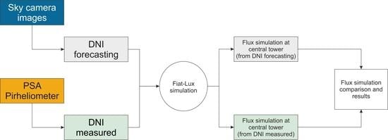
2.6. Fiat-Lux Simulation

After the DNI on the ground has been predicted using the method developed for the sky camera, the next step consists of analyzing the losses in the path between the heliostats (on the ground) and the receiver (on top of the central tower). The main idea is to control the primary errors resulting from the simulation process for predicting the DNI on the tower’s receiver.

Normally, the optical losses are computerized using past data and a model able to control enough of the variables involved in characterizing the sunlight’s path [26,27]. In this work, the flux density, in W/m${}^2$ is predicted on the tower receiver (located 82 m above ground level) using the predicted DNI data and the Fiat-Lux model [28]. Fiat-Lux is a ray-tracing code developed in Matlab© environment by PSA in 1977 for simulating the optics of heliostat prototypes and later extended to heliostat fields. Its main feature is that it uses a real sunshape as input signal in the sun specular reflection process on the heliostat surface. The sunshape picture is captured by a high resolution imaging device and transformed in a matrix representative of the relative gray-scale sun intensity. The known spatial calibration of the camera, i.e., angle subtended by adjacent pixels, plus the simultaneous measurement of a pyrheliometer, provide a sun image whose pixels are calibrated both geometrically and in terms of direct solar irradiance coming from the solar disk. This calibrated sunshape matrix is projected onto the target by a previously modeled heliostat reflecting surface, following the reflection law. For a single heliostat the reflecting surface is initially modeled using 11 parameters enough to describe morphology, geometry and mirror waviness. This heliostat was selected from the CESA-I PSA solar field, and consists of a 39.9 m${}^2$ twelve-facet heliostat with a focal distance of 260 m and a solar weighted reflectance of 0.94. The final projection of the sun shape reflected by the mirror is made using the ray-tracing technique. After applying the Fiat-Lux code, an estimation of the total irradiance distribution reaching the receiver is obtained.

3. Results

In this section, we present the DNI prediction results for the central tower receiver at the CESA-1 plant. The total flux on the PSA’s central tower receiver was predicted for different time intervals, following the purpose of this work to include the DNI forecasting, from the TSI images, in the Fiat-Lux model, to compare the predictions with real DNI values. As the DNI forecasting from the TSI-880 is performed up until 120 min, at one-minute intervals, we carried out the flux prediction for 30, 60 and 120 min, as representative meteorological prevision values.

To be able to perform the ray tracing correctly, the sun’s position at instant m (at which the prediction is made) is taken into account. In this work, different moments have been simulated, with different solar altitudes, over two full days, where the DNI prediction method is combined with the flow modeling in the tower using the Fiat-Lux model. Specifically, the days of 9 and 10 March 2017 were analyzed.

Since the purpose of this work is to quantify the error propagation of the methods used for predicting the flux on the tower receiver, two consecutive cloudless days at the PSA were selected as the most appropriate for these studies; this is because atmospheric attenuation is easier to identify under clear sky conditions than under overcast skies, avoiding uncertainties provide by clouds, like prediction, composition, etc. The 9 and 10 March 2017 were considered cloudless according to the DNI curves, as they appear in Figure 4.

Therefore, the first step is to determine the DNI forecasting at ground level using the sky camera. To analyze how successful the DNI prediction at the PSA is (from 1 to 120 min), certain statistical indicators were used, such as the normalized mean bias error (Equation (2)), the normalized root-mean-square error (Equation (3)) and the correlation coefficient (Equation (4)), used in different studies [14,22,24].

Therefore, the first step consisted in the determination of the DNI forecasting at ground level using the sky camera. For analyzing the success of the DNI prediction in the PSA (from 1 to 120 min), some statistical indicators, like normalized mean bias error (Equation (2)), normalized root-mean-square error (Equation (3)) and correlation coefficient (Equation (4)), were used

$$nMBE(\%)=[(\frac{\frac{1}{N}{\displaystyle \sum _{i=1}^N}(DN{I}_{est}-DN{I}_{mea})}{DN{I}_{max}-DN{I}_{min}})100]$$

(2)

where N is the number of cases studied, DNI${}_{est}$ is the estimated DNI, DNI${}_{mea}$ is the measured DNI, DNI${}_{max}$ represents the maximum DNI value and DNI${}_{min}$ the minimum from the measured values.

$$nRMSE(\%)=[(\frac{\sqrt{\frac{1}{N}{\displaystyle \sum _{i=1}^N}{(DN{I}_{est}-DN{I}_{mea})}^2}}{DN{I}_{max}-DN{I}_{min}})100]$$

(3)

$$r=\frac{{\sigma }_{DN{I}_{est}DN{I}_{mea}}}{{\sigma }_{DN{I}_{est}}{\sigma }_{DN{I}_{mea}}},$$

(4)

where ${\sigma }_{DN{I}_{est}DN{I}_{mea}}$ is the covariance of the two input data sets (the estimated and measured DNI), and ${\sigma }_{DN{I}_{est}}$ and ${\sigma }_{DN{I}_{mea}}$ are the covariances of the estimated and measured DNI, respectively. According to this,

Table 3. Statistical errors of DNI forecasting on the ground for the two cloudless days selected.

Forecast Time	nMBE (%)	nRMSE (%)	r
1 min	−10.73	14.63	0.92
30 min	−9.62	15.74	0.87
60 min	−7.70	17.52	0.77
120 min	−2.68	21.60	0.54

shows the results of the DNI forecasting.

The DNI forecasting results at ground level present values below 20% nRMSE for all the predictions, except that for 120 min, which increases a little. Furthermore, the nMBE shows that the DNI is always underestimated, with values lower than 10% approximately, whereas the r-value shows that the DNI is predicted with an r-value of 0.97 for one minute and 0.87 for 30 min. As shown, the nMBE is higher in the first minute than for 120 min, the reason being that, in this temporal horizon, the prediction gives a higher underestimation that is not easy to solve due to the saturation of pixels in the sun area.

Given the high computational cost of simulating the ray tracing, simulations have been performed using the estimated and predicted DNI values. Specifically, for March 9th, the predictions were carried out at 9:02 UTC (Universal Time Coordinated) and 12:02 UTC, with time horizons at 1, 30, 60 and 120 min. For each prediction time, rays were plotted according to the sun’s position, the reference heliostat and the focal point located in the central tower. Figure 5 and Figure 6 show the different scenarios analyzed for 9 March 2017.

In each of the figures presented (Figure 5 and Figure 6), there are four different scenarios. Each scenario shows the ray-tracing simulation from the time the sun hits the reference heliostat until it is projected onto the focal point of the tower’s receiver. Initially, the prediction is made a minute before the time of the first scenario; for example, for Figure 5, all the predictions are made at 9:02 UTC, with the first prediction being minute 1 (9:03 UTC), the second being minute 30 (9:32 UTC) and so on, for all the scenarios and figures presented. Moreover, for each prediction time, the flux distribution at the focal point has been calculated, using the actual irradiance and the irradiance predicted by the sky camera. Specifically, an example can be seen in Figure 7, where the irradiance predicted at 120 min from the sky cam was used in the simulation.

As one can observe, the concentration of the rays forms a non-perfect circle, with different irradiance levels depending on their position with respect to the center; these are expressed on a scale in kW/m${}^2$. Figure 8 shows the horizontal and vertical flux distribution for the analyzed case in more detail, according to the proximity to the center of the concentration.

As a graph, one can see how the irradiance is higher than 8 kW/m${}^2$ at the center of the focal point, while lower at the ends, thus forming a Gaussian bell with the center at 0 m.

Furthermore, the day of 10 March 2017 was studied to quantify the prediction at the flux focus under a clear sky. In this case, three times of the day were set: 7:17, 9:07 and 12:02 UTC. For each time, predictions were made from 1 min to 120 min, simulating the projections with actual and predicted irradiance values to observe the differences. Figure 9, Figure 10 and Figure 11 show the different scenarios analyzed for 10 March 2017.

In these images, and in the scenarios analyzed, one can see how the position of the sun varies throughout the day and how it influences the ray tracing from the heliostat to the focal point located on the central tower at CESA-1. Figure 12 shows the flux distribution on the target located at the top of the tower, 259.53 m from the reference heliostat, for the prediction made at 9:07 UTC for 2 h ahead (11:07 UTC).

The concentration differs from that seen in Figure 7, as the ellipse is defined in another direction, according to the sun’s position with respect to the reference heliostat and the tower. Figure 13 shows the horizontal and vertical flux distribution for the analyzed case in more detail.

As one can observe, the plots showing the flux distribution on the two axes are quite similar and are only conditioned by the level of concentrated irradiance, which is why only two specific cases have been presented from all the simulations.

Subsequently, for each minute of prediction, we obtained a flux value on the receiver that compared with the flux value should the real DNI have been used. For each prediction, several variables were obtained, such as the predicted and measured DNI, the predicted and real total available power (PTAP and RTAP, respectively) at ground, the predicted and real total power on target (PTPT and RTPT, respectively), the average cosine factor (ACF), the predicted irradiance peak (PIP) and the real irradiance peak (RIP).

Table 4. Representation of the results obtained during the experiment performed in the solar field at the PSA, where the first column represents the date and hour of the prediction and the second column shows the time of the prediction; the other columns represent the numerical variables considered in the study. DNI predicted and DNI measured (in W/m${}^2$), the predicted and real total available power (PTAP and RTAP, respectively) at ground, the predicted and real total power on target (PTPT and RTPT, respectively), the average cosine factor (ACF), the predicted irradiance peak (PIP) and the real irradiance peak (RIP).

Date of Prediction	Forecast Time (UTC)	DNI Predicted (W/m${}^2$)	DNI Measured (W/m${}^2$)	PTAP (kW)	RTAP (kW)	PTPT (kW)	RTPT (kW)	ACF	PIP (kW/m${}^2$)	RIP (kW/m${}^2$)
9 March	1 min	849.9	912.0	33.7	36.7	28.9	31.1	0.86	7.5	8.1
2017	30 min	848.0	949.0	33.6	37.6	29.5	33.0	0.88	7.7	8.6
9:02	60 min	846.0	975.0	33.6	38.7	30.0	34.6	0.89	8.9	9.1
	120 min	845.5	1004.0	33.5	39.8	31.0	36.6	0.92	8.1	9.7
9 March	1 min	862.0	1015.0	34.2	40.3	31.9	37.5	0.93	8.4	9.9
2017	30 min	861.0	1013.0	34.2	40.2	31.9	37.5	0.93	8.4	9.9
12:02	60 min	860.9	1008.0	34.2	39.9	31.8	37.2	0.93	8.4	9.8
	120 min	861.0	993.0	34.5	39.4	31.4	36.2	0.92	8.3	9.5
10 March	1 min	826.0	659.0	32.8	26.1	25.3	20.2	0.78	6.3	5.0
2017	30 min	826.3	798.2	32.8	31.7	26.2	25.3	0.80	6.6	6.4
7:17	60 min	826.0	881.0	32.8	35.0	27.0	28.8	0.82	6.9	7.4
	120 min	826.0	983.0	32.8	39.0	28.4	33.8	0.87	7.4	8.8
10 March	1 min	851.8	973.0	33.8	38.6	29.1	33.2	0.86	7.6	8.6
2017	30 min	851.8	1002.0	33.8	39.8	29.7	35.0	0.88	7.8	9.1
7:17	60 min	851.8	1024.0	33.8	40.6	30.3	36.4	0.90	7.9	9.5
	120 min	851.8	1051.0	33.8	41.7	31.1	38.3	0.92	8.2	10.1
10 March	1 min	863.6	1057.0	34.3	41.9	31.9	39.0	0.93	8.4	10.3
2017	30 min	863.6	1056.0	34.3	41.9	31.9	39.0	0.93	8.4	10.3
7:17	60 min	863.6	1052.0	34.3	41.7	31.9	38.8	0.93	8.4	10.2
	120 min	863.6	1028.0	34.3	40.8	31.4	37.4	0.92	8.3	9.9

summarizes the values obtained in the experiment carried out at the PSA site on 9 and 10 March 2017, in which we have analyzed moments with low solar altitude angles (early moments) and high altitude angles (midday approximately).

These insolation levels are translated into total available power, depending on the heliostat properties, where the predicted and real values follow the same trend as the DNI. By multiplying the available power and the ACF values, the power on target is obtained. This variable represents the amount of insolation that reaches the target/receiver of the central tower. In our case, the best results are presented for the first prediction minute on 9 March, where the difference between the real and predicted potential in the receiver is below 8%.

In all the situations, the predicted DNI is always underestimated, as one can clearly see. This means the predicted PTAP values are always lower than the RTAP values by approximately 12%, matching the percentage difference between the average PIP and RIP values. However, the difference between the PTPT and RTPT values increases slightly, to 16%, probably due to the standard deviation that may occur in the simulation model, which in this case is approximately 4.0%.

Normally, the predicted values are lower than the measured values due to several processes, except at the early moments, as can be seen in the first predictions at 7:17 on 10 March, when the solar altitude was 9°. In this moment, there is a peak, but it is demonstrable that the predictions work better with higher solar altitudes (normally above 10–15°) [22]. For the other cases, we can observe that, as with the other variables, the differences between the predicted and real power on target are always below 20%. Finally, the irradiance peak allows us to quantify the peak of insolation that reaches the receiver (per square meter). This value is very important for determining the distribution of the heliostat reflection on the volumetric receiver. In this case, the values vary from 5.0 to 10.3 kW/m${}^2$ if the real flux is used, and from 6.3 to 8.9 if the radiation is predicted. In these situations, the difference between the measured and predicted values is also below 20%.

Consequently, a model has been developed for predicting the flux on the target of a central tower, detailing the differences that can occur in a prediction system when estimating and predicting the solar resource, and when simulating the flux in the central tower. For all cases, the difference was in the 12 to 16% range for clear sky conditions and for different solar heights on the same day.

4. Conclusions

In this work, we have presented the results of an experiment carried out at the PSA site to predict the flux on the receiver of the central tower. Two cloudless days were selected: 9 and 10 March 2017.

A model TSI-880 sky camera was installed in the PSA solar field to predict the short-term DNI (nowcasting). The DNI was estimated and predicted using the maximum cross-correlation method and the digital image levels. Specifically, the prediction was made for several moments of the days, from one to 120 min, at one-minute intervals. To do this, the sun area pixels were used to obtain the future radiation at ground level in real time. In this work, periods of 1, 30, 60 and 120 min were used.

To project the DNI reaching the central tower receiver from the ground, the Fiat-Lux model was employed to determine the sun’s trajectory and optical losses. Subsequently, the experiment involved the simulation of the flux value on the receiver. In this way, real and forecasted power-on-target values have been compared, by means of the combination of a total sky camera and Fiat-Lux ray-tracing model.

Analyzing the results, we can state that the nRMSE differences between the real measured values and those obtained from the sky camera predictions are below 16% for 30 min of prediction. For the total available power and peak irradiance predictions, the average difference between the actual and predicted values is 12% from 1 min to 120 min, while the Fiat-Lux simulation represents a 4% deviation over the value predicted with the TSI-880 camera.

To summarize, in this work, we have defined a novel combination of solar irradiance forecasting (using sky cams) and flux simulation in a CSTP plant environment. It has been possible to work with real data from a ground-level DNI prediction, which has served as input for flux simulations at a central tower receiver. We have detailed the steps and numerical statistical errors that occur when predicting the solar flux on the receiver. To improve this process, the next step would be to include mechanisms for detecting atmospheric attenuation, which would help to optimize DNI forecasting techniques.

References

1. Chapman, A.J.; McLellan, B.C.; Tezuka, T. Prioritizing mitigation efforts considering co-benefits, equity and energy justice: Fossil fuel to renewable energy transition pathways. Appl. Energy 2018, 219, 187–198. [Google Scholar] [CrossRef]
2. Li, H.; Edwards, D.; Hosseini, M.; Costin, G. A review on renewable energy transition in Australia: An updated depiction. J. Clean. Prod. 2020, 242, 118475. [Google Scholar] [CrossRef]
3. Lovegrove, K.; Stein, W. Concentrating Solar Power Technology: Principles, Developments and Applications; Woodhead Publishing: Sawston, UK, 2012; pp. 1–674. [Google Scholar]
4. Petrík, T.; Daneček, M.; Uhlíř, I.; Poulek, V.; Libra, M. Distribution Grid Stability—Influence of Inertia Moment of Synchronous Machines. Appl. Sci. 2020, 10, 9075. [Google Scholar] [CrossRef]
5. Ferro, G.; Robba, M.; Sacile, R. A Model Predictive Control Strategy for Distribution Grids: Voltage and Frequency Regulation for Islanded Mode Operation. Energies 2020, 13, 2637. [Google Scholar] [CrossRef]
6. Lubkoll, M.; Erasmus, D.; Harms, T.; von Backström, T.; Kröger, D. Performance characteristics of the Spiky Central Receiver Air Pre-heater (SCRAP). Sol. Energy 2020, 201, 773–786. [Google Scholar] [CrossRef] [Green Version]
7. Ballestrín, J.; Marzo, A. Solar radiation attenuation in solar tower plants. Sol. Energy 2012, 86, 388–392. [Google Scholar] [CrossRef]
8. Hanrieder, N.; Wilbert, S.; Pitz-Paal, R.; Emde, C.; Gasteiger, J.; Mayer, B.; Polo, J. Atmospheric extinction in solar tower plants: Absorption and broadband correction for MOR measurements. Atmos. Meas. Tech. 2015, 8, 3467–3480. [Google Scholar] [CrossRef] [Green Version]
9. López, G.; Gueymard, C.A.; Bosch, J.L.; Rapp-Arrarás, I.; Alonso-Montesinos, J.; Pulido-Calvo, I.; Ballestrín, J.; Polo, J.; Barbero, J. Modelling water vapor impact on the solar energy reaching the receiver of a solar tower plant by means of artificial neural networks. Sol. Energy 2016, 165, 34–39. [Google Scholar]
10. Blanco, M.J.; Mutuberria, A.; Martínez, D. Experimental validation of Tonatiuh using the Plataforma Solar de Almería secondary concentrator test campaign data. In Proceedings of the 16th Annual SolarPACES Symposium, Perpignan, France, 21–24 September 2010. [Google Scholar]
11. Polo, J.; Ballestrín, J.; Carra, E. Sensitivity study for modelling atmospheric attenuation of solar radiation with radiative transfer models and the impact in solar tower plant production. Sol. Energy 2016, 134, 219–227. [Google Scholar] [CrossRef]
12. Mondragón, R.; Alonso-Montesinos, J.; Riveros-Rosas, D.; Bonifaz, R. Determination of cloud motion applying the Lucas-Kanade method to sky cam imagery. Remote Sens. 2020, 12, 2643. [Google Scholar] [CrossRef]
13. Masuda, R.; Iwabuchi, H.; Schmidt, K.; Damiani, A.; Kudo, R. Retrieval of cloud optical thickness from sky-view camera images using a deep convolutional neural network based on three-dimensional radiative transfer. Remote Sens. 2019, 11, 1962. [Google Scholar] [CrossRef] [Green Version]
14. Alonso, J.; Batlles, F.J. The use of a sky camera for solar radiation estimation based on digital image processing. Energy 2015, 90, 377–386. [Google Scholar] [CrossRef]
15. Mommert, M. Cloud Identification from All-sky Camera Data with Machine Learning. Astron. J. 2020, 159, 4. [Google Scholar] [CrossRef]
16. Alonso-Montesinos, J. Real-time automatic cloud detection using a low-cost sky camera. Remote Sens. 2020, 12, 1382. [Google Scholar] [CrossRef]
17. Ballestrín, J.; Monterreal, R.; Carra, M.; Fernández-Reche, J.; Polo, J.; Enrique, R.; Rodríguez, J.; Casanova, M.; Barbero, F.; Alonso-Montesinos, J.; et al. Solar extinction measurement system based on digital cameras. Application to solar tower plants. Renew. Energy 2018, 125, 648–654. [Google Scholar] [CrossRef]
18. Alonso, J.; Batlles, F.J.; López, G.; Ternero, A. Sky camera imagery processing based on a sky classification using radiometric data. Energy 2014, 68, 599–608. [Google Scholar] [CrossRef]
19. Chu, Y.; Li, M.; Coimbra, C. Sun-tracking imaging system for intra-hour DNI forecasts. Renew. Energy 2016, 96, 792–799. [Google Scholar] [CrossRef]
20. Dev, S.; Savoy, F.; Hui Lee, Y.; Winkler, S. Estimating solar irradiance using sky imagers. Atmos. Meas. Tech. 2019, 12, 5417–5429. [Google Scholar] [CrossRef] [Green Version]
21. Rajagukguk, R.A.; Kamil, R.; Lee, H.J. A Deep Learning Model to Forecast Solar Irradiance Using a Sky Camera. Appl. Sci. 2021, 11, 5049. [Google Scholar] [CrossRef]
22. Alonso-Montesinos, J.; Batlles, F.; Portillo, C. Solar irradiance forecasting at one-minute intervals for different sky conditions using sky camera images. Energy Convers. Manag. 2015, 105, 1166–1177. [Google Scholar] [CrossRef]
23. Bone, V.; Pidgeon, J.; Kearney, M.; Veeraragavan, A. Intra-hour direct normal irradiance forecasting through adaptive clear-sky modelling and cloud tracking. Sol. Energy 2018, 159, 852–867. [Google Scholar] [CrossRef]
24. Alonso, J.; Batlles, F.J.; Villarroel, C.; Ayala, R.; Burgaleta, J.I. Determination of the sun area in sky camera images using radiometric data. Energy Convers. Manag. 2014, 78, 24–31. [Google Scholar] [CrossRef]
25. Alonso-Montesinos, J.; Batlles, F.J. Short and medium-term cloudiness forecasting using remote sensing techniques and sky camera imagery. Energy 2014, 73, 890–897. [Google Scholar] [CrossRef]
26. Sánchez-González, A.; Santana, D. Solar flux distribution on central receivers: A projection method from analytic function. Renew. Energy 2015, 74, 576–587. [Google Scholar] [CrossRef]
27. He, C.; Zhao, H.; He, Q.; Zhao, Y.; Feng, J. Analytical radiative flux model via convolution integral and image plane mapping. Energy 2021, 222, 119937. [Google Scholar] [CrossRef]
28. Monterreal, R. A new computer code for solar concentrating optics simulation. J. Phys. 1999, 9, 77–82. [Google Scholar] [CrossRef]
Figure 1. The TSI-880 sky camera placed at the northern end of the PSA site.
Remotesensing 14 01602 g001
Figure 2. Flowchart of the process used for the DNI forecasting at the PSA site.
Remotesensing 14 01602 g002
Figure 3. Representation of the CMV determination in each sector of the sky-camera image.
Remotesensing 14 01602 g003
Figure 4. DNI measured on 9 and 10 March 2017 at the PSA site.
Remotesensing 14 01602 g004
Figure 5. Scheme of the DNI forecasting simulation on the target (9 March 2017 at 12:02 UTC).
Remotesensing 14 01602 g005
Figure 6. Scheme of simulation for DNI forecasting on target (9 March 2017 at 12:02 UTC).
Remotesensing 14 01602 g006
Figure 7. Flux distribution on the target (9 March 2017 at 14:02 UTC).
Remotesensing 14 01602 g007
Figure 8. Vertical and horizontal flux profile on the target (9 March 2017 at 14:02 UTC).
Remotesensing 14 01602 g008
Figure 9. Scheme of the DNI forecasting simulation on the target (10 March 2017 at 7:17 UTC).
Remotesensing 14 01602 g009
Figure 10. Scheme of the DNI forecasting simulation on the target (10 March 2017 at 9:07 UTC).
Remotesensing 14 01602 g010
Figure 11. Scheme of the DNI forecasting simulation on the target (10 March 2017 at 12:02 UTC).
Remotesensing 14 01602 g011
Figure 12. Flux distribution on the target (10 March 2017 at 11:07 UTC).
Remotesensing 14 01602 g012
Figure 13. Vertical and horizontal flux profile on the target (10 March 2017 at 11:07 UTC).
Remotesensing 14 01602 g013