
The Staring Mode Properties and Performance of Geo-SAR Satellite with Reflector Antenna

Abstract
:
1. Introduction
- ◼
- Staring mode imaging range mainly depends on a beam’s 3 dB coverage scale. Geo-SAR can constantly obtain a scene range of 320 km × 320 km in the whole orbit through a 25 m aperture circular antenna.
- ◼
- The Geo-SAR staring mode aims to obtain constantly an azimuth resolution of 25 m in different orbit positions through partial synthetic aperture.
- ◼
- A new two-dimensional pitch and roll squint controlling (2D-PRSC) method is proposed. The beam can quickly point to any area of 320 km × 320 km distributed in a zone of 5000 km × 5000 km. The satellite’s maneuver monitoring capability is promoted due to its attitude controlling angles being less than ±7.6 degrees. The time and energy expended for attitude controlling can be significantly saved.
- ◼
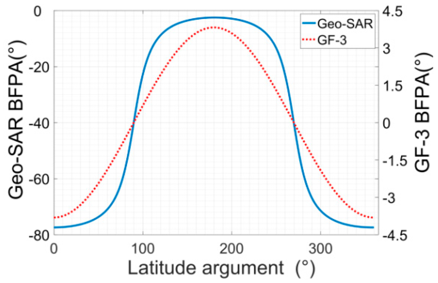
- Due to the distinct variation of the beam footprint direction angle (BFPA) caused by the satellite’s periodic large yaw angle, CASR also needs to be considered as well as AASR and RASR. Furthermore, it is necessary to analyze its ambiguity in the whole orbital period because of Geo-SAR’s strong time-varying velocity.
2. Attitude Controlling Technology
2.1. Satellite Attitude Characteristic
2.2. 2D-PRSC Technology for Squint Staring Mode
2.2.1. Large Instantaneous Field of View for Geo-SAR
2.2.2. 2D-PRSC Theory Illumination
- (a)
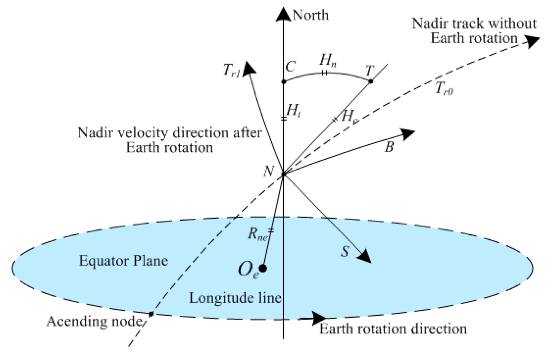
- Calculating the original GSA.
- (b)
- Calculating the target direction angle. It is defined as the angle between the meridian and the line between the nadir and scene center.
- (c)
- Pitch and roll angle’s expressions are derived. The satellite can stare at a fixed scene by controlling these two angles.
- (d)
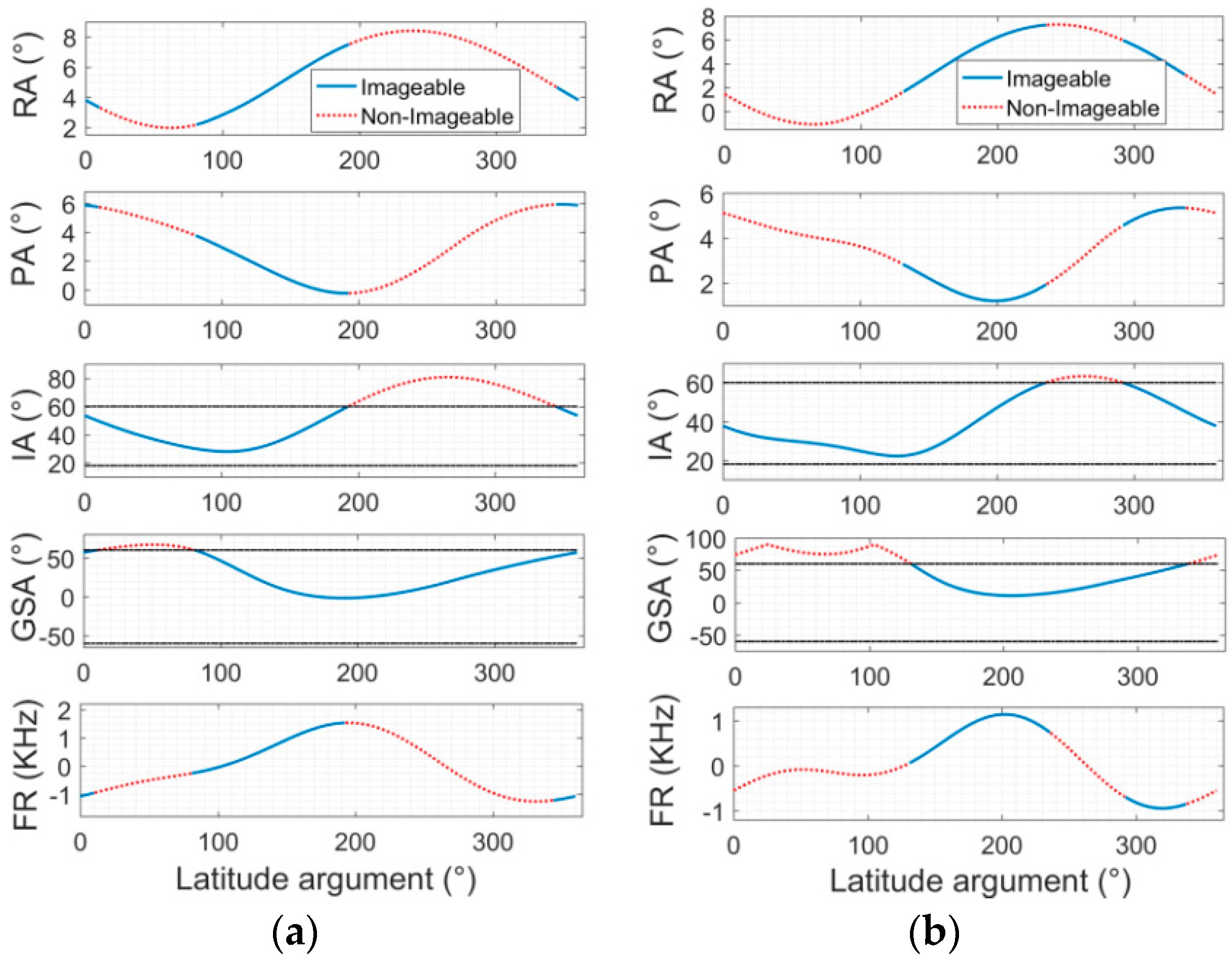
- Whether the current orbital segment meets the imaging conditions or not is confirmed according to the GSA and incidence angle (IA) threshold constraints.
2.2.3. Simulation
3. Staring Imaging Mode
3.1. Geo-SAR Staring Mode Model and Characteristics
- ◼
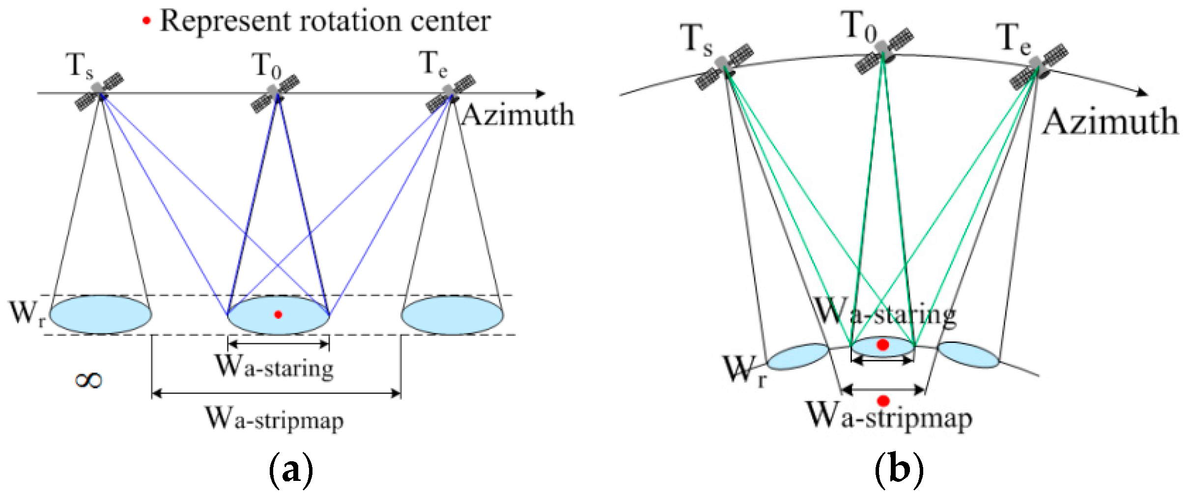
- Geo-SAR’s stripmap mode is similar to Leo-SAR’s slide spotlight mode. Since Geo-SAR satellite’s speed is about seven times its beam’s moving speed, the rotation center is not at infinity, as Leo-SAR is in the stripmap mode condition. However, both of their rotation centers are in the scene center in the staring mode condition, as shown in Figure 8.
- ◼
- Geo-SAR’s azimuth imaging scale is mainly determined by its beam coverage. The staring mode is recommended to select, and the azimuth imaging scale is always equal to the beam coverage during its orbital period.
- ◼
- Leo-SAR just needs one-dimensional azimuth beam direction controlling; however, Geo-SAR needs a more complicated two-dimensional beam direction controlling algorithm to realize the staring mode. The theory in Section 2 has illustrated the 2D-PRSC method for squint staring (broadside is a special case of squint).
- ◼
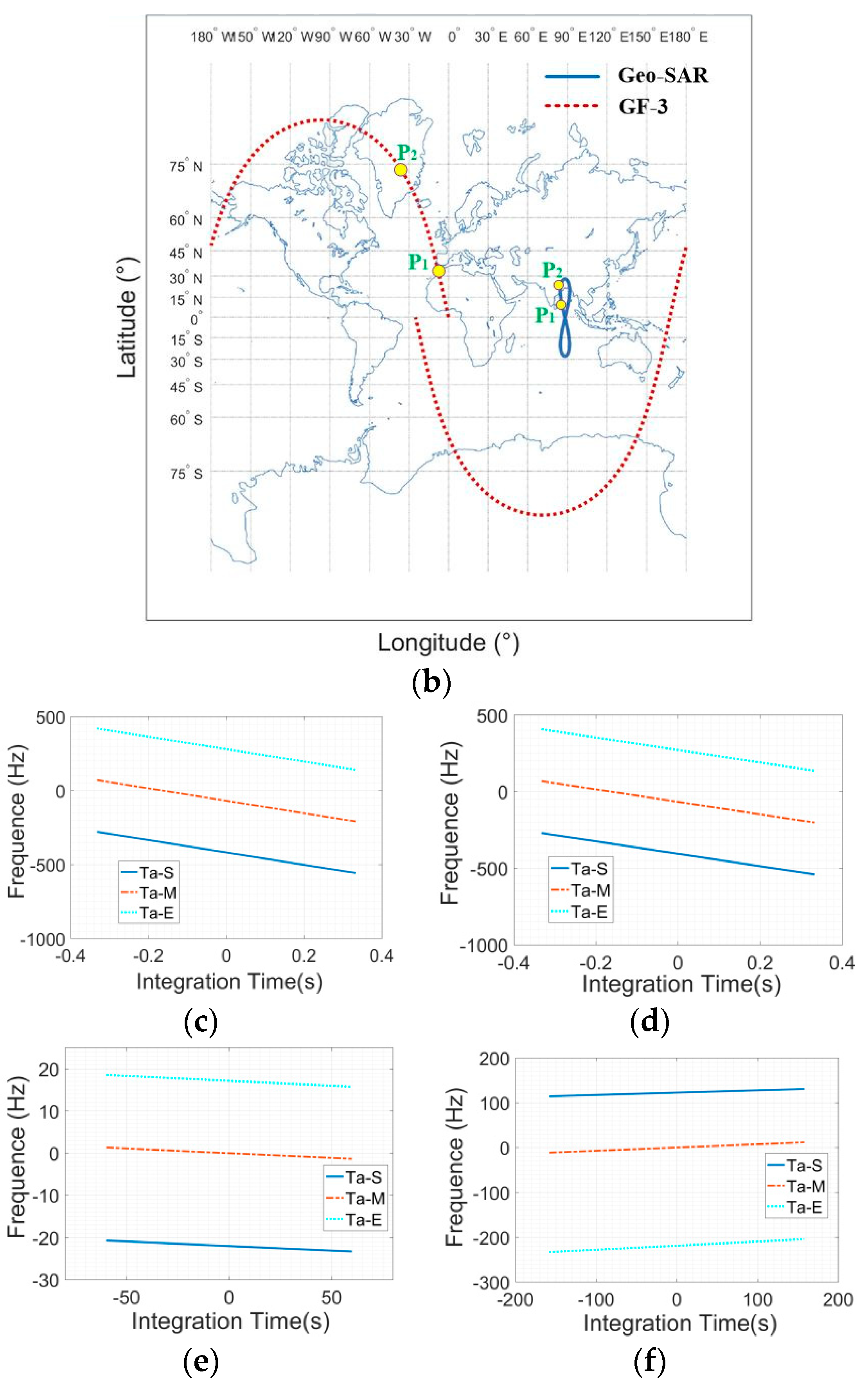
- The Geo-SAR Doppler FM rate, positive or negative, always changes during the whole orbit. Its staring mode Doppler history is also strongly time-varying. The Leo-SAR Doppler FM rate, almost unchanged, is negative in the whole orbit, and its Doppler history hardly changes. Figure 9a compares the Doppler FM rate of Geo-SAR and GF-3 in the same IA of 45.5 degrees. The Doppler FM rate of Geo-SAR is (−0.11, 0.1) Hz/s, and that of GF-3 is (−1680, −1618) Hz/s. Furthermore, considering the orbital symmetry, a latitude argument of 23.4 degrees and 75.7 degrees, marked by P1 and P2, are selected to compare the two satellites’ staring mode Doppler history. Figure 9b–f show the simulation results. The Doppler history of the starting, middle, and terminal point targets of the staring area are, respectively, represented by Ta-S, Ta-M, and Ta-E, which are marked by different colors and lines. Unlike GF-3, Geo-SAR Doppler history has a strong time-varying property, as listed in Table 2. In addition, the Doppler frequency interval between Ta-S, Ta-M, and Ta-E of Geo-SAR is not uniform, and it changes obviously with the latitude argument. This is also quite different from Leo-SAR.
3.2. Antenna and Power
3.2.1. Antenna Selection
3.2.2. Antenna Shape and Area
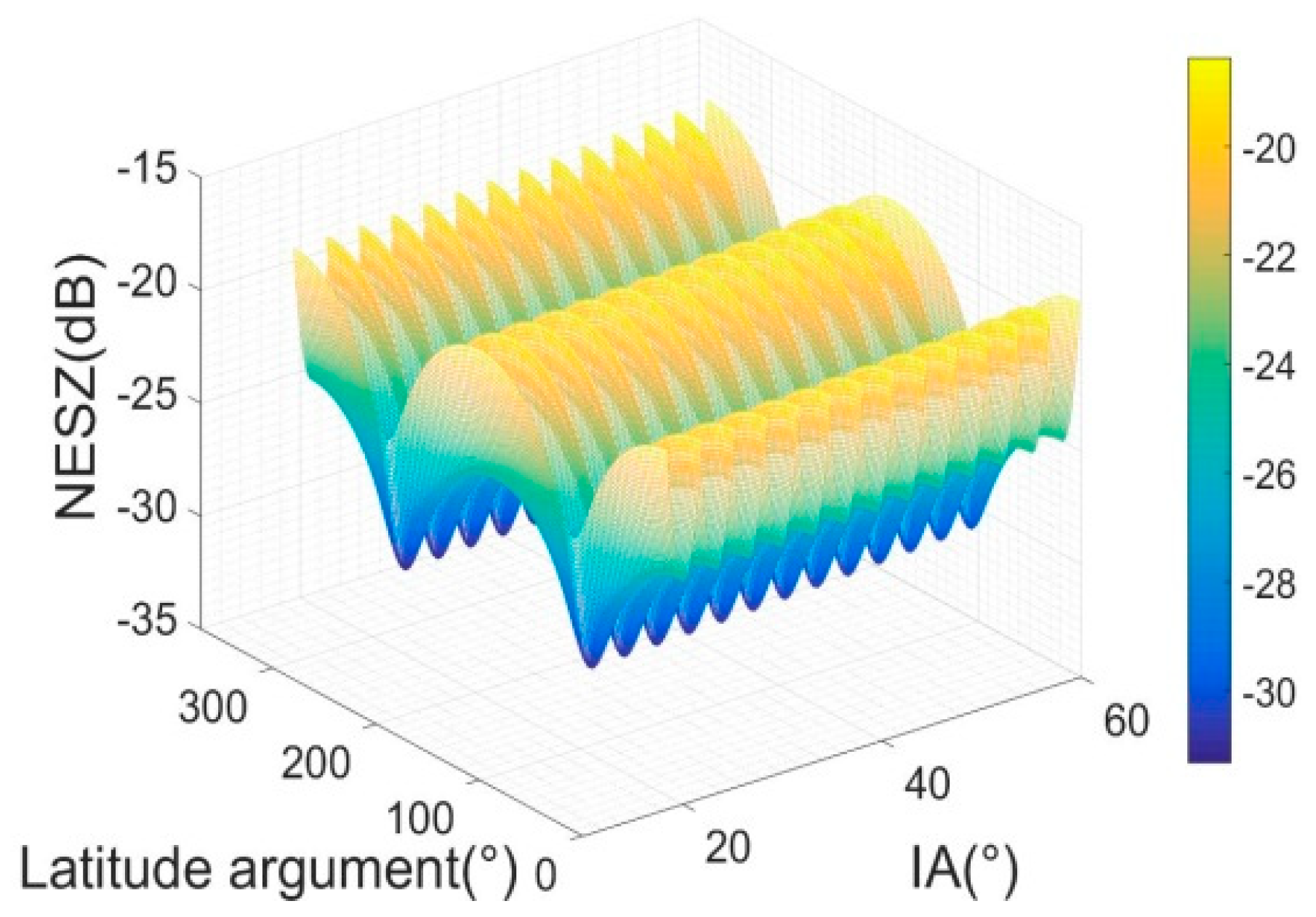
3.2.3. NESZ
4. Ambiguity Analysis
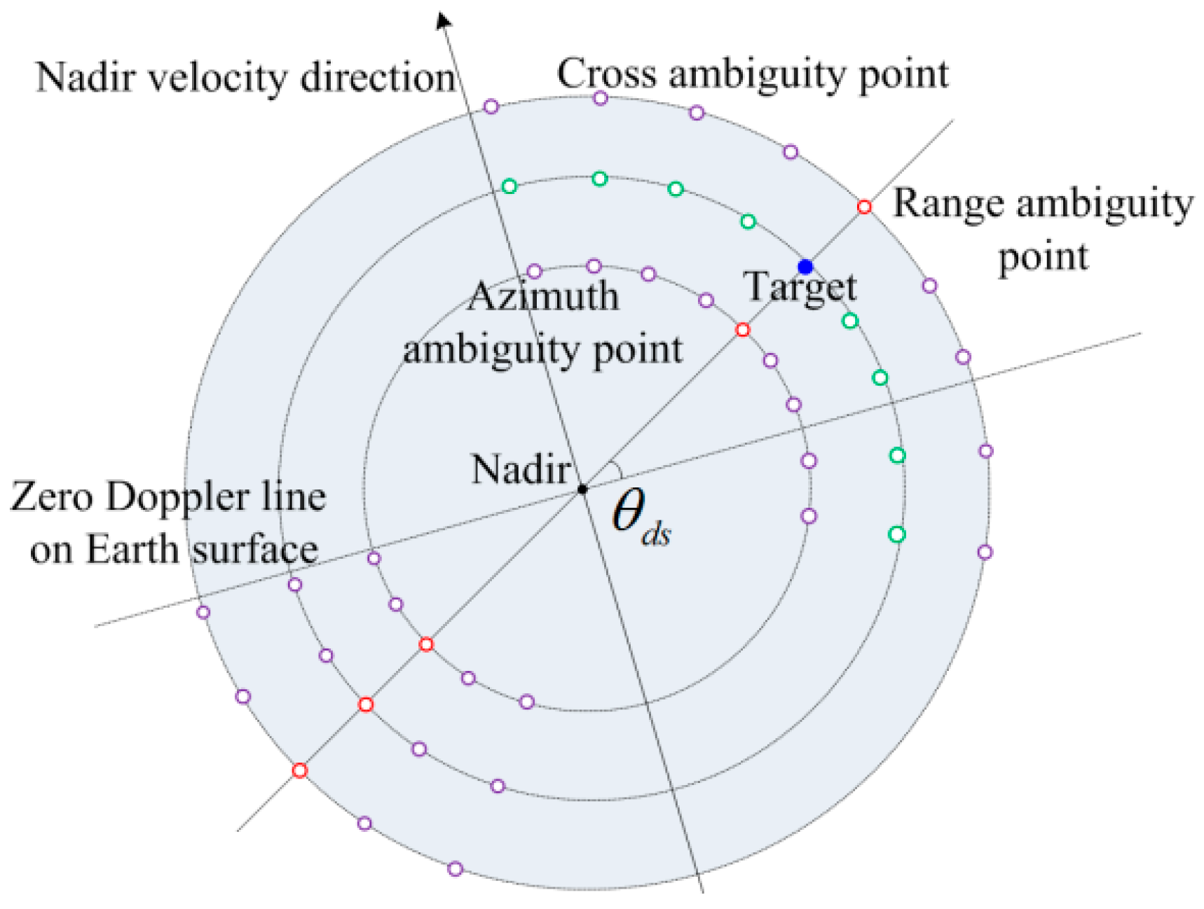
4.1. Geo-SAR Staring Mode Ambiguity Model
- ◼
- RASR: those with the same Doppler frequency as signal (i.e., m = 0 and n ≠ 0 in (31));
- ◼
- AASR: those along the same slant range as signal (i.e., m ≠ 0 and n = 0 in (31));
- ◼
- CASR: the remaining terms (i.e., m ≠ 0 and n ≠ 0 in (31)).
- ◼
- It is necessary to use a two-dimensional antenna pattern to calculate ASR; otherwise, the error will be very large;
- ◼
- The ASR of Geo-SAR is obtained in 2D-PRSC conditions. This calculation result is quite different from that in 2D-YS conditions.
- ◼
- Due to the influence of the large BFPA, the CASR of Geo-SAR cannot be ignored for system designing;
- ◼
- Geo-SAR usually works in the squint condition for emergency missions. So, it is necessary to consider both GSA and BFPA to obtain the ambiguity point location. This further increases the ASR calculation complexity.
- ◼
- RASR, AASR, and CASR of Geo-SAR are all strongly time-varying. As a result, whole orbital ergodic analysis is necessary in system designing process.
4.2. RASR
4.3. DT-AASR
4.4. DT-CASR
4.5. Simulation Results
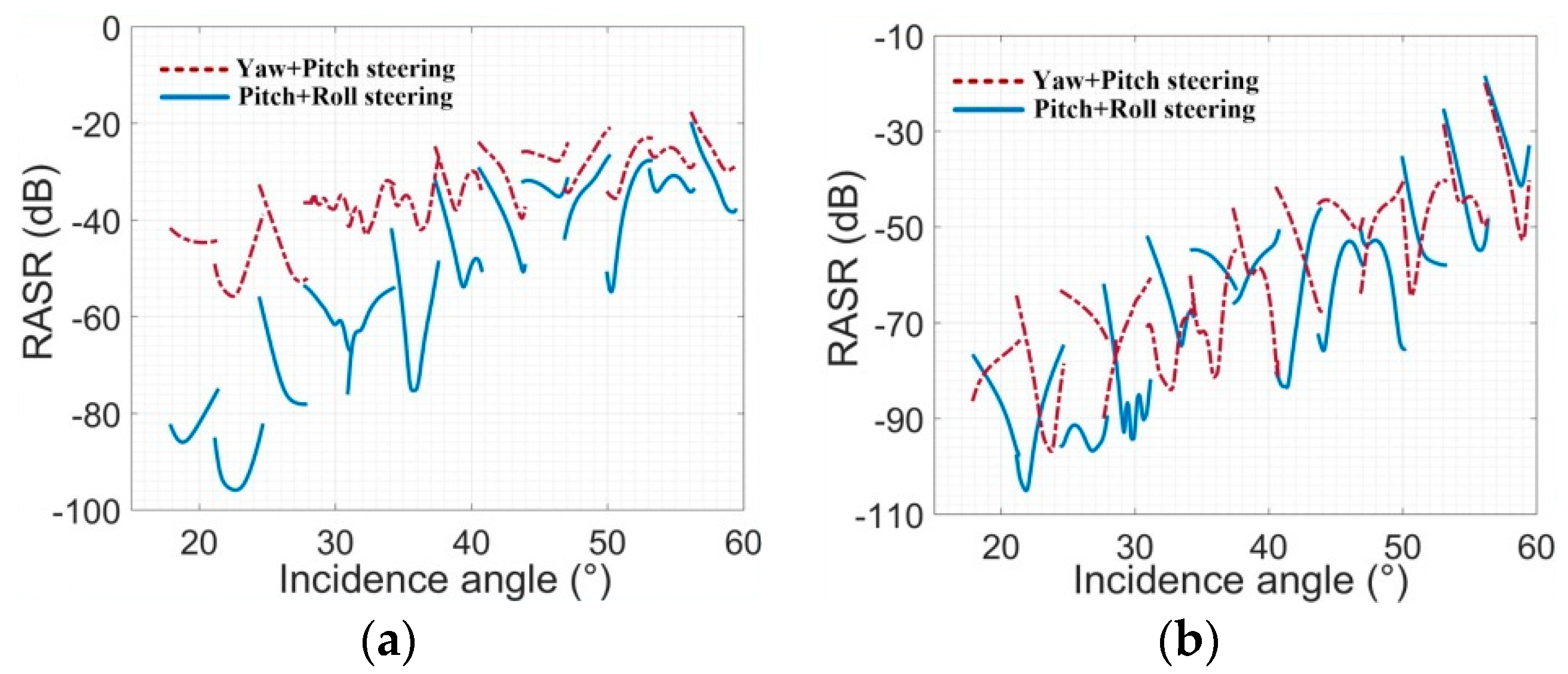
4.5.1. RASR
- ◼
- In broadside condition, RASR in the 2D-PRSC condition is about 2–45 dB better than that in the 2D-YS condition. The smaller the incidence angle is, the greater the improvement. Due to BFPA, not all the antenna elevation pattern gain is in the range of the ambiguity region. So, the range ambiguity signal is weakened.
- ◼
- In the squint condition, the differences of RASR between the different attitude steering methods are not obvious. This is because that BFPA, which is about −72 degrees at a latitude argument of 23.4 degrees, counteracts most of the antenna elevation pattern gain variety caused by GSA.
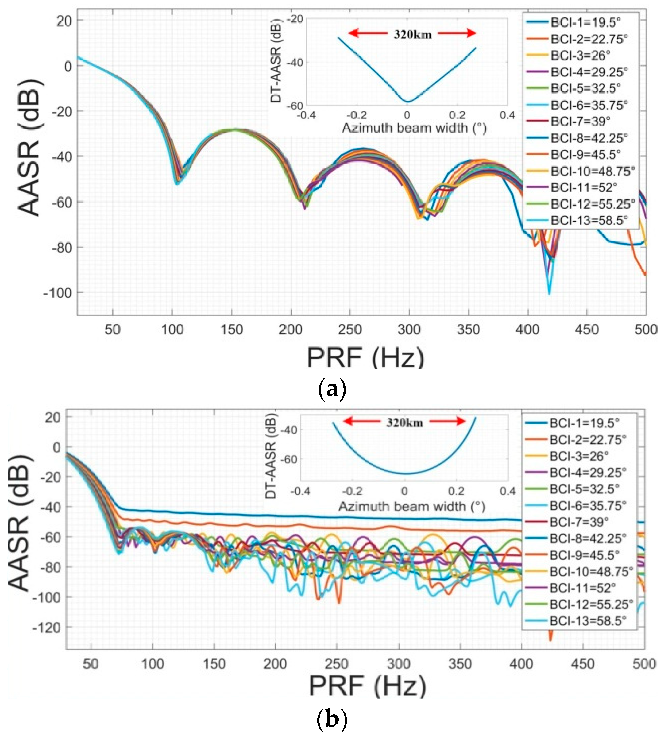
4.5.2. DT-AASR
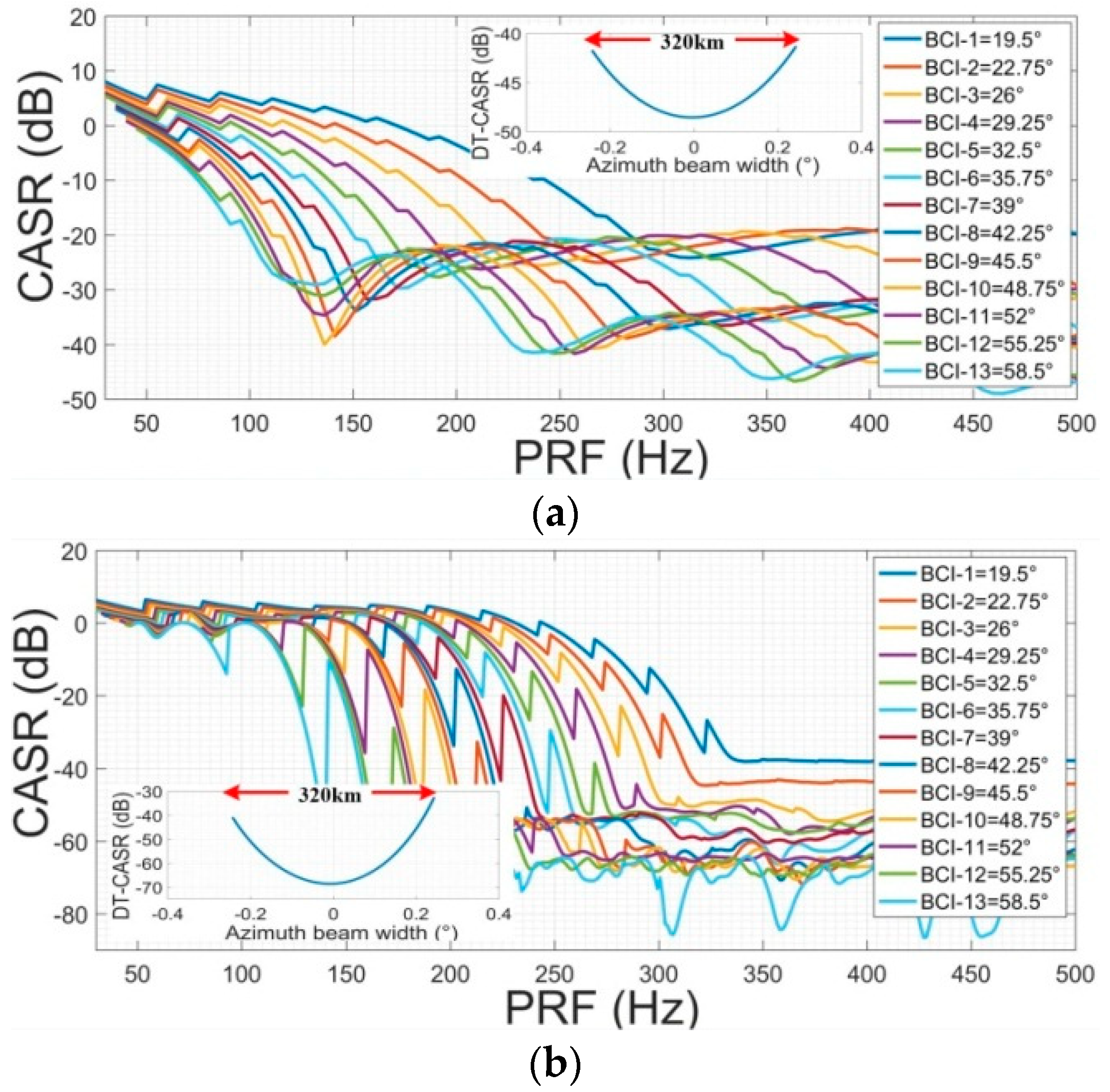
4.5.3. DT-CASR
- ◼
- CASR has a comparable magnitude as AASR in the Geo-SAR condition, so it cannot be ignored. The constraints of RASR, AASR, and CASR should be considered simultaneously in the process of system designing.
- ◼
- Due to the strong time-varying property, different GSA and latitude argument both have obvious effects on AASR and CASR. Therefore, the GSA should be calculated according to the longitude and latitude of the expected imaging zone and satellite’s position. Furthermore, it is recommended to recalculate and update the system parameters for every five-degree change in latitude argument.
- ◼
- The DT-AASR and DT-CASR of the distributed targets in the azimuth range change significantly for the staring mode. In order to ensure that the DT-AASR and DT-CASR of all targets in the azimuth range of 320 km meet the requirement of −20 dB, it is necessary to select an appropriate PRF in the scale of (160, 430) Hz.
- ◼
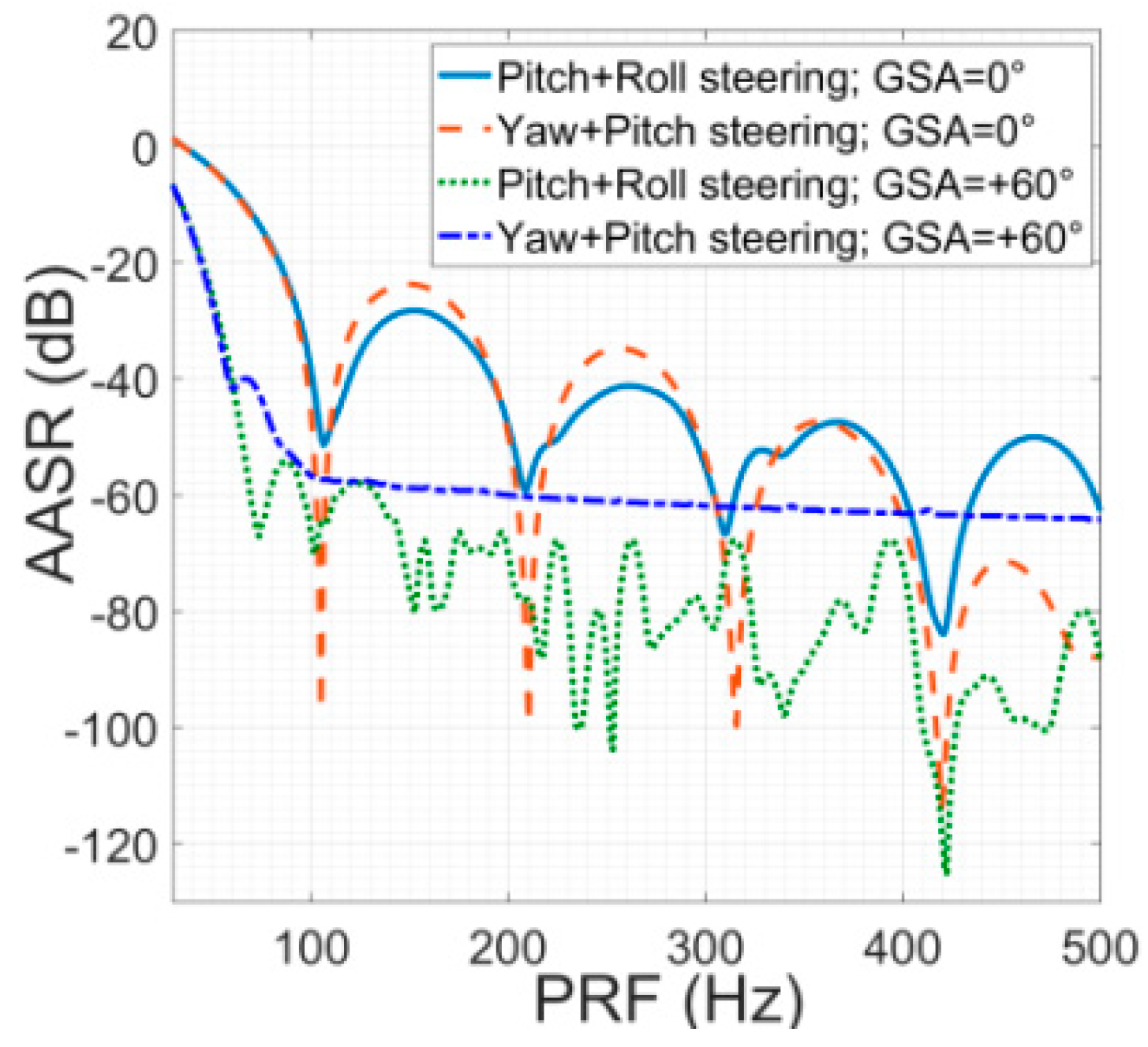
- Different from RASR, the influence of different attitude steering methods on AASR and CASR is not obvious.
5. Conclusions
Author Contributions
Funding
Conflicts of Interest
References
- Tomiyasu, K. Synthetic aperture radar in geosynchronous orbit. In Proceedings of the Digest International IEEE Antennas Propagation Symposium, College Park, MD, USA, 15–19 May 1978; pp. 42–45. [Google Scholar]
- Tomiyasu, K.; Pacelli, J.L. Synthetic aperture radar imaging from an inclined geosynchronous orbit. IEEE Trans. Geosci. Remote Sens. 1983, GE-21, 324–329. [Google Scholar] [CrossRef]
- Long, T.; Hu, C.; Ding, Z.; Dong, X.; Tian, W.; Zeng, T. Geosynchronous SAR: System and Signal Processing; Springer: Singapore, 2018. [Google Scholar] [CrossRef]
- Matar, J.; Rodriguez-Cassola, M.; Krieger, G.; López-Dekker, P.; Moreira, A. MEO SAR: System concepts and analysis. IEEE Trans. Geosci. Remote Sens. 2019, 58, 1313–1324. [Google Scholar] [CrossRef] [Green Version]
- Hobbs, S.; Sanchez, J.P. Laplace plane and low inclination geosynchronous radar mission design. Sci. China Inf. Sci. 2017, 60, 060305. [Google Scholar] [CrossRef]
- Zhang, Y.; Xiong, W.; Dong, X.; Hu, C.; Sun, Y. GRFT-based moving ship target detection and imaging in geosynchronous SAR. Remote Sens. 2018, 10, 2002. [Google Scholar] [CrossRef] [Green Version]
- Global Earthquake Satellite System: A 20-Year Plan to Enable Earthquake Prediction; JPL Document: Pasadena, CA, USA, 2003.
- Zhou, B.; Qi, X.; Zhang, J.; Zhang, H. Effect of 6-DOF Oscillation of Ship Target on SAR Imaging. Remote Sens. 2021, 13, 1821. [Google Scholar] [CrossRef]
- Bingji, Z.; Qingun, Z.; Chao, D.; Weiping, S.; MingMing, X. Baseline designing and implementation approach for a Geo-SAR tomography system. J. Eng. 2019, 2019, 6235–6238. [Google Scholar] [CrossRef]
- Zhao, B.; Zhang, Q.; Dai, C.; Liu, L. Baseline Accuracy Analysis for Sub-Geosynchronous Orbital Tomo-SAR System. In Proceedings of the 2019 6th Asia-Pacific Conference on Synthetic Aperture Radar (APSAR), Xiamen, China, 26–29 November 2019; pp. 1–4. [Google Scholar]
- Prati, C.; Rocca, F.; Giancola, D.; Guarnieri, A.M. Passive geosynchronous SAR system reusing backscattered digital audio broadcasting signals. IEEE Trans. Geosci. Remote Sens. 1998, 36, 1973–1976. [Google Scholar] [CrossRef] [Green Version]
- Guarnieri, A.M.; Leanza, A.; Recchia, A.; Tebaldini, S.; Venuti, G. Atmospheric Phase Screen in GEO-SAR: Estimation and Compensation. IEEE Trans. Geosci. Remote Sens. 2017, 56, 1668–1679. [Google Scholar] [CrossRef]
- Chen, J.; Sun, G.-C.; Xing, M.; Yang, J.; Ni, C.; Zhu, Y.; Shu, W.; Liu, W. A Parameter Optimization Model for Geosynchronous SAR Sensor in Aspects of Signal Bandwidth and Integration Time. IEEE Geosci. Remote Sens. Lett. 2016, 13, 1374–1378. [Google Scholar] [CrossRef]
- Hobbs, S.; Mitchell, C.; Forte, B.; Holley, R.; Snapir, B.; Whittaker, P. System Design for Geosynchronous Synthetic Aperture Radar Missions. IEEE Trans. Geosci. Remote Sens. 2014, 52, 7750–7763. [Google Scholar] [CrossRef] [Green Version]
- Hu, C.; Long, T.; Liu, Z.; Zeng, T.; Tian, Y. An Improved Frequency Domain Focusing Method in Geosynchronous SAR. IEEE Trans. Geosci. Remote Sens. 2013, 52, 5514–5528. [Google Scholar] [CrossRef]
- Wang, R.; Hu, C.; Li, Y.; Hobbs, S.E.; Tian, W.; Dong, X.; Chen, L. Joint Amplitude-Phase Compensation for Ionospheric Scintillation in GEO SAR Imaging. IEEE Trans. Geosci. Remote Sens. 2017, 55, 3454–3465. [Google Scholar] [CrossRef]
- Zhang, T.; Ding, Z.; Tian, W.; Zeng, T.; Yin, W. A 2-D Nonlinear Chirp Scaling Algorithm for High Squint GEO SAR Imaging Based on Optimal Azimuth Polynomial Compensation. IEEE J. Sel. Top. Appl. Earth Obs. Remote Sens. 2017, 10, 5724–5735. [Google Scholar] [CrossRef]
- Rodon, J.R.; Broquetas, A.; Monti-Guarnieri, A.V.; Rocca, F. Geosynchronous SAR Focusing With Atmospheric Phase Screen Retrieval and Compensation. IEEE Trans. Geosci. Remote Sens. 2013, 51, 4397–4404. [Google Scholar] [CrossRef]
- Zheng, W.; Hu, J.; Zhang, W.; Yang, C.; Li, Z.; Zhu, J. Potential of geosynchronous SAR interferometric measurements in estimating three-dimensional surface displacements. Sci. China Inf. Sci. 2017, 60, 060304. [Google Scholar] [CrossRef]
- Recchia, A.; Monti-Guarnieri, A.V.; Broquetas, A.; Leanza, A. Impact of Scene Decorrelation on Geosynchronous SAR Data Focusing. IEEE Trans. Geosci. Remote Sens. 2015, 54, 1635–1646. [Google Scholar] [CrossRef] [Green Version]
- Cumming, I.G.; Wong, F.H. Digital Processing of Synthetic Aperture Radar Data: Algorithms and Implementation; Artech House: Boston, MA, USA, 2005; pp. 90–152. [Google Scholar]
- Davidson, G.W.; Cumming, I. Signal properties of spaceborne squint-mode SAR. IEEE Trans. Geosci. Remote Sens. 1997, 35, 611–617. [Google Scholar] [CrossRef] [Green Version]
- Li, G.; Fang, S.; Han, B.; Zhang, Z.; Hong, W.; Wu, Y. Compensation of Phase Errors for Spotlight SAR With Discrete Azimuth Beam Steering Based on Entropy Minimization. IEEE Geosci. Remote Sens. Lett. 2020, 18, 841–845. [Google Scholar] [CrossRef]
- Prats-Iraola, P.; Scheiber, R.; Mittermayer, J.; Meta, A.; Moreira, A. Processing of Sliding Spotlight and TOPS SAR Data Using Baseband Azimuth Scaling. IEEE Trans. Geosci. Remote Sens. 2009, 48, 770–780. [Google Scholar] [CrossRef] [Green Version]
- Meta, A.; Mittermayer, J.; Prats, P.; Scheiber, R.; Steinbrecher, U. TOPS imaging with TerraSAR-X: Mode design and performance analysis. IEEE Trans. Geosci. Remote Sens. 2009, 48, 759–769. [Google Scholar] [CrossRef] [Green Version]
- De Zan, F.; Guarnieri, A.M. TOPSAR: Terrain observation by progressive scans. IEEE Trans. Geosci. Remote Sens. 2006, 44, 2352–2360. [Google Scholar] [CrossRef]
- Sacco, P.; Battagliere, M.L.; Coletta, A. COSMO-SKYMED mission status: Results, lessons learnt and evolutions. In Proceedings of the 2015 IEEE International Geoscience and Remote Sensing Symposium (IGARSS), Milan, Italy, 26–31 July 2015; pp. 207–210. [Google Scholar]
- Pastina, D.; Turin, F. Exploitation of the COSMO-SkyMed SAR system for GMTI applications. IEEE J. Sel. Top. Appl. Earth Obs. Remote Sens. 2014, 8, 966–979. [Google Scholar] [CrossRef]
- Potin, P.; Rosich, B.; Miranda, N.; Grimont, P.; Shurmer, I.; O’Connell, A.; Krassenburg, M.; Gratadour, J.-B. Copernicus Sentinel-1 Constellation Mission Operations Status. In Proceedings of the IEEE International Geosciences and Remote Sensing Symposium, Yokohama, Japan, 28 July–2 August 2019; pp. 5385–5388. [Google Scholar] [CrossRef]
- Benedetti, A.; Picchiani, M.; Del Frate, F. Sentinel-1 and Sentinel-2 Data Fusion for Urban Change Detection. In Proceedings of the IGARSS 2018-2018 IEEE International Geoscience and Remote Sensing Symposium, Valencia, Spain, 22–27 July 2018; pp. 1962–1965. [Google Scholar] [CrossRef]
- Liang, D.; Zhang, H.; Fang, T.; Deng, Y.; Yu, W.; Zhang, L.; Fan, H. Processing of Very High Resolution GF-3 SAR Spotlight Data With Non-Start–Stop Model and Correction of Curved Orbit. IEEE J. Sel. Top. Appl. Earth Obs. Remote Sens. 2020, 13, 2112–2122. [Google Scholar] [CrossRef]
- Mittermayer, J.; Wollstadt, S.; Prats-Iraola, P.; Scheiber, R. The TerraSAR-X staring spotlight mode concept. IEEE Trans. Geosci. Remote Sens. 2013, 52, 3695–3706. [Google Scholar] [CrossRef]
- Kraus, T.; Bräutigam, B.; Grigorov, C.; Mittermayer, J.; Wollstadt, S. TerraSAR-X staring spotlight mode optimization. In Proceedings of the 2013 Asia-Pacific Conference on Synthetic Aperture Radar (APSAR), Tsukuba, Japan, 23–27 September 2013; pp. 16–19. [Google Scholar]
- Jordan, R.L. The Seasat-A synthetic aperture radar system. IEEE J. Ocean. Eng. 1980, 5, 154–164. [Google Scholar] [CrossRef]
- Raney, R.K. Doppler properties of radars in circular orbits. Int. J. Remote Sens. 1986, 7, 1153–1162. [Google Scholar] [CrossRef]
- Fiedler, H.; Boerner, E.; Mittermayer, J.; Krieger, G. Total zero Doppler steering-a new method for minimizing the Doppler centroid. IEEE Geosci. Remote Sens. Lett. 2005, 2, 141–145. [Google Scholar] [CrossRef]
- Ze, Y.; Yinqing, Z.; Jie, C.; Chunsheng, L. A new satellite attitude steering approach for zero Doppler centroid. In Proceedings of the IET International Radar Conference, Guilin, China, 20–22 April 2009; pp. 1–4. [Google Scholar]
- Zhang, J.; Yu, Z.E.; Xiao, P. A novel antenna beam steering strategy for GEO SAR staring observation. In Proceedings of the 2016 IEEE International Geoscience and Remote Sensing Symposium (IGARSS), Beijing, China, 10–15 July 2016; pp. 1106–1109. [Google Scholar]
- Long, T.; Dong, X.; Hu, C.; Zeng, T. A new method of zero-Doppler centroid control in GEO SAR. IEEE Geosci. Remote Sens. Lett. 2010, 8, 512–516. [Google Scholar] [CrossRef]
- Jiang, Y.; Hu, B.; Zhang, Y.; Lian, M.; Wang, Z. Study on Zero-Doppler Centroid Control for GEO SAR Ground Observation. Int. J. Antennas Propag. 2014, 2014, 549269. [Google Scholar] [CrossRef]
- Guarnieri, A.M. Adaptive removal of azimuth ambiguities in SAR images. IEEE Trans. Geosci. Remote Sens. 2005, 43, 625–633. [Google Scholar] [CrossRef]
- Li, F.K.; Johnson, W.T.K. Ambiguities in spacebornene synthetic aperture radar systems. IEEE Trans. Aerosp. Electron. Syst. 1983, 3, 389–397. [Google Scholar] [CrossRef]
- Villano, M.; Krieger, G.; Moreira, A. New insights into ambiguities in quad-pol SAR. IEEE Trans. Geosci. Remote Sens. 2017, 55, 3287–3308. [Google Scholar] [CrossRef]
- Huber, S.; de Almeida, F.Q.; Villano, M.; Younis, M.; Krieger, G.; Moreira, A. Tandem-L: A technical perspective on future spaceborne SAR sensors for Earth observation. IEEE Trans. Geosci. Remote Sens. 2018, 56, 4792–4807. [Google Scholar] [CrossRef] [Green Version]


| Name | GF-3 | Geo-SAR |
|---|---|---|
| Semi-major axis (km) | 7126.4 | 42,163.5 |
| Inclination angle (°) | 98.4 | 28 |
| Eccentricity | 0.001 | 0.001 |
| Incidence angle (°) | 45.5 | 45.5 |
| Argument of perigee (°) | 90 | 90 |
| Wave length (m) | 0.06 | 0.24 |
| Earth model | WSG84 | WSG84 |
| Name | GF-3 | Geo-SAR | ||
|---|---|---|---|---|
| Latitude argument (°) | 23.4 | 75.7 | 23.4 | 75.7 |
| Azimuth resolution (m) | 1 | 1 | 25 | 25 |
| Integration time (s) | 0.57 | 0.58 | 115.8 | 311.2 |
| Doppler bandwidth (Hz) | 1075.2 | 1043.5 | 46.1 | 400.7 |
| Parameter Name | Value | Parameter Name | Value |
|---|---|---|---|
| Semi-major axis (km) | 42,163.5 | Wave length (m) | 0.24 |
| Argument of perigee (°) | 90 | Inclination (°) | 28 |
| Range swath width (km) | ≥320 | Bandwidth (MHz) | 50 |
| Incidence angle (°) | (18, 60) | Eccentricity | 0.001 |
| Ground squint angle (°) | 0/60 | Earth model | WSG84 |
| Azimuth resolution (m) | 25 | Antenna size (m) | 25 |
| Ground range resolution (m) | 25 | Latitude argument (°) | 23.4 |
Publisher’s Note: MDPI stays neutral with regard to jurisdictional claims in published maps and institutional affiliations. |
© 2022 by the authors. Licensee MDPI, Basel, Switzerland. This article is an open access article distributed under the terms and conditions of the Creative Commons Attribution (CC BY) license (https://creativecommons.org/licenses/by/4.0/).
Share and Cite
Zhao, B.; Zhang, Q. The Staring Mode Properties and Performance of Geo-SAR Satellite with Reflector Antenna. Remote Sens. 2022, 14, 1609. https://doi.org/10.3390/rs14071609
Zhao B, Zhang Q. The Staring Mode Properties and Performance of Geo-SAR Satellite with Reflector Antenna. Remote Sensing. 2022; 14(7):1609. https://doi.org/10.3390/rs14071609
Chicago/Turabian StyleZhao, Bingji, and Qingjun Zhang. 2022. "The Staring Mode Properties and Performance of Geo-SAR Satellite with Reflector Antenna" Remote Sensing 14, no. 7: 1609. https://doi.org/10.3390/rs14071609