
Measuring Coastal Subsidence after Recent Earthquakes in Chile Central Using SAR Interferometry and GNSS Data


Abstract
:1. Introduction
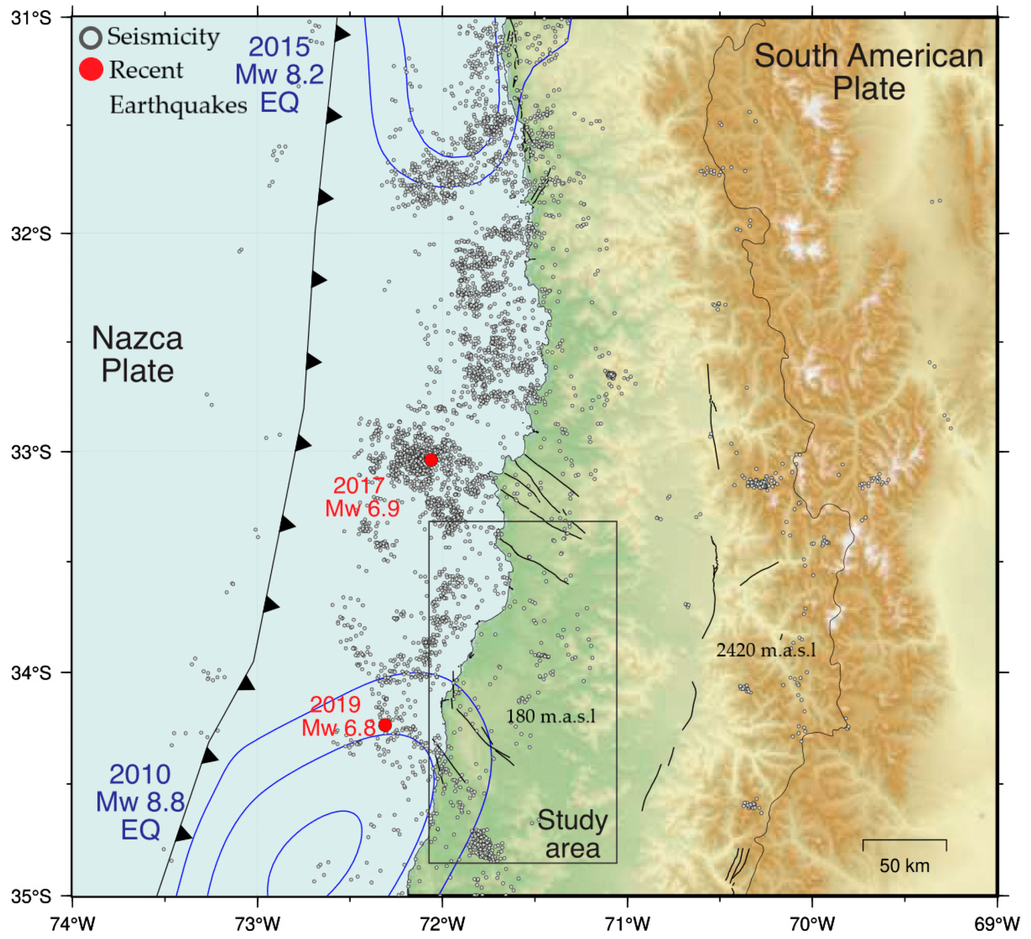
2. Study Area
Geological Setting
3. Materials and Methods
3.1. Data Set: SAR Imagery
3.2. GNSS Data
3.3. P-SBAS Processing
3.4. Post-Processing
Vertical and East-West Deformation Component Estimation
4. Results and Discussion
4.1. Regional Displacement Overview
4.2. Subsidence Area
4.2.1. Time Series Verification
4.2.2. Vertical Displacement Estimation
4.2.3. E-W Displacement Estimation
4.3. Urban Areas
5. Conclusions
Supplementary Materials
Author Contributions
Funding
Institutional Review Board Statement
Informed Consent Statement
Data Availability Statement
Acknowledgments
Conflicts of Interest
References
- Scholz, C.H. The Mechanics of Earthquakes and Faulting; Cambridge University Press: Cambridge, UK, 2002; pp. 300–329. [Google Scholar]
- DeMets, C.; Gordon, R.G.; Argus, D.F.; Stein, S. Effects of recent revision to the geomagnetic reversal timescale on estimates of current plate motion. Geophys. Res. Lett. 1994, 21, 2191–2194. [Google Scholar] [CrossRef]
- Moreno, M.; Rosenau, M.; Oncken, O. Maule earthquake slip correlates with pre-seismic locking of Andean subduction zone. Nature 2010, 467, 198–202. [Google Scholar] [CrossRef] [PubMed]
- Bedford, J.; Moreno, M.; Baez, J.C.; Lange, D.; Tilmann, F.; Rosenau, M.; Heidbach, O.; Oncken, O.; Bartsch, M.; Rietbrock, A.; et al. A high-resolution, time-variable afterslip model for the 2010 Maule Mw = 8.8, Chile megathrust earthquake. Earth Planet. Sci. Lett. 2013, 383, 26–36. [Google Scholar] [CrossRef] [Green Version]
- Kelson, K.; Witter, R.C.; Tassara, A.; Ryder, I.; Ledezma, C.; Montalva, G.; Frost, D.; Sitar, N.; Moss, R.; Johnson, L. Coseismic Tectonic Surface Deformation during the 2010 Maule, Chile, Mw 8.8 Earthquake. Earthq. Spectra 2012, 28, 39–54. [Google Scholar] [CrossRef]
- Vargas, G.; Farías, M.; Carretier, S.; Tassara, A.; Baize, S.; Melnick, D. Coastal uplift and tsunami effects associated to the 2010 Mw8. 8 Maule earthquake in Central Chile. Andean Geol. 2011, 38, 219–238. [Google Scholar]
- Cecioni, A.; Pineda, V. Geology and Geomorphology of Natural Hazards and Humand-Induced Disasters in Chile; Latrubesse, E., Ed.; Elsevier: Amsterdam, The Netherlands, 2009; pp. 379–412. [Google Scholar]
- Watts, A.B. Tectonic subsidence, flexure and global changes of sea level. Nature 1982, 297, 469–474. [Google Scholar] [CrossRef]
- Dokka, R.K. Modern-day tectonic subsidence in coastal Louisiana. Geology 2006, 34, 281–284. [Google Scholar] [CrossRef]
- Minderhoud, P.; Middelkoop, H.; Erkens, G.; Stouthamer, E. Groundwater extraction may drown mega-delta: Projections of extraction-induced subsidence and elevation of the Mekong delta for the 21st century. Environ. Res. Commun. 2019, 2, 011005. [Google Scholar] [CrossRef]
- Chen, B.; Gong, H.; Chen, Y.; Li, X.; Zhou, C.; Lei, K.; Zhu, L.; Duan, L.; Zhao, X. Land subsidence and its relation with groundwater aquifers in Beijing Plain of China. Sci. Total Environ. 2020, 735, 139111. [Google Scholar] [CrossRef]
- Guo, L.; Gong, H.; Ke, Y.; Zhu, L.; Li, X.; Lyu, M.; Zhang, K. Mechanism of Land Subsidence Mutation in Beijing Plain under the Background of Urban Expansion. Remote Sens. 2021, 13, 3086. [Google Scholar] [CrossRef]
- Turner, R.E.; Mo, Y. Salt Marsh Elevation limit determined after subsidence from hydrologic change and hydro-carbon extraction. Remote Sens. 2021, 13, 49. [Google Scholar] [CrossRef]
- Singh, A.; Rao, G.S. Crustal structure and subsidence history of the Mannar basin through potential field modelling and backstripping analysis: Implications on basin evolution and hydrocarbon exploration. J. Pet. Sci. Eng. 2021, 206, 109000. [Google Scholar] [CrossRef]
- Gahramanov, G.; Babayev, M.; Shpyrko, S.; Mukhtarova, K. Subsidence history and hydrocarbon migration modeling in south caspian basin. Visnyk Taras Shevchenko Natl. Univ. Kyiv. Geol. 2020, 1, 82–91. [Google Scholar] [CrossRef]
- Stramondo, S.; Bozzano, F.; Marra, F.; Wegmuller, U.; Cinti, F.; Moro, M.; Saroli, M. Subsidence induced by urbanisation in the city of Rome detected by advanced InSAR technique and geotechnical investigations. Remote Sens. Environ. 2008, 112, 3160–3172. [Google Scholar] [CrossRef]
- Manunta, M.; Marsella, M.; Zeni, G.; Sciotti, M.; Atzori, S.; Lanari, R. Two-scale surface deformation analysis using the SBAS-DInSAR technique: A case study of the city of Rome, Italy. Int. J. Remote Sens. 2008, 29, 1665–1684. [Google Scholar] [CrossRef]
- Abidin, H.Z.; Andreas, H.; Djaja, R.; Darmawan, D.; Gamal, M. Land subsidence characteristics of Jakarta between 1997 and 2005, as estimated using GPS surveys. GPS Solut. 2008, 12, 23–32. [Google Scholar] [CrossRef]
- Orellana, F.; Blasco, J.D.; Foumelis, M.; D’Aranno, P.; Marsella, M.; Di Mascio, P. DInSAR for Road Infrastructure Monitoring: Case Study Highway Network of Rome Metropolitan (Italy). Remote Sens. 2020, 12, 3697. [Google Scholar] [CrossRef]
- Chang, L.; Dollevoet, R.P.B.J.; Hanssen, R.F. Monitoring Line-Infrastructure with Multisensor SAR Interferometry: Products and Performance Assessment Metrics. IEEE J. Sel. Top. Appl. Earth Obs. Remote Sens. 2018, 11, 1593–1605. [Google Scholar] [CrossRef] [Green Version]
- Ferretti, A.; Fumagalli, A.; Novali, F.; Prati, C.; Rocca, F.; Rucci, A. A New Algorithm for Processing Interferometric Data-Stacks: SqueeSAR. IEEE Trans. Geosci. Remote Sens. 2011, 49, 3460–3470. [Google Scholar] [CrossRef]
- Ferretti, A.; Prati, C.; Rocca, F. Nonlinear subsidence rate estimation using permanent scatterers in differential SAR interferometry. IEEE Trans. Geosci. Remote Sens. 2000, 38, 2202–2212. [Google Scholar] [CrossRef] [Green Version]
- Lanari, R.; Mora, O.; Manunta, M.; Mallorqui, J.J.; Berardino, P.; Sansosti, E. A small-baseline approach for investigating deformations on full-resolution differential SAR interferograms. IEEE Trans. Geosci. Remote Sens. 2004, 42, 1377–1386. [Google Scholar] [CrossRef]
- Werner, C.; Wegmuller, U.; Strozzi, T.; Wiesmann, A. Interferometric point target analysis for deformation mapping. In Proceedings of the International Geoscience and Remote Sensing symposium (IGARSS), Toulouse, France, 21–25 July 2003; Volume 7, pp. 4362–4364. [Google Scholar]
- Bonano, M.; Manunta, M.; Pepe, A.; Paglia, L.; Lanari, R. From Previous C-Band to New X-Band SAR Systems: Assessment of the DInSAR Mapping Improvement for Deformation Time-Series Retrieval in Urban Areas. IEEE Trans. Geosci. Remote Sens. 2013, 51, 1973–1984. [Google Scholar] [CrossRef]
- Casu, F.; Manzo, M.; Lanari, R. A quantitative assessment of the SBAS algorithm performance for surface deformation retrieval from DInSAR data. Remote Sens. Environ. 2006, 102, 195–210. [Google Scholar] [CrossRef]
- Crosetto, M.; Monserrat, O.; Cuevas, M.; Crippa, B. Spaceborne Differential SAR Interferometry: Data Analysis Tools for Deformation Measurement. Remote Sens. 2011, 3, 305–318. [Google Scholar] [CrossRef] [Green Version]
- Bovenga, F.; Nitti, D.O.; Fornaro, G.; Radicioni, F.; Stoppini, A.; Brigante, R. Using C/X-band SAR interferometry and GNSS measurements for the Assisi landslide analysis. Int. J. Remote Sens. 2013, 34, 4083–4104. [Google Scholar] [CrossRef]
- Hilley, G.E.; Bürgmann, R.; Ferretti, A.; Novali, F.; Rocca, F. Dynamics of Slow-Moving Landslides from Permanent Scatterer Analysis. Science 2004, 304, 1952–1955. [Google Scholar] [CrossRef] [Green Version]
- Sansosti, E.; Casu, F.; Manzo, M.; Lanari, R. Space-borne radar interferometry techniques for the generation of deformation time series: An advanced tool for Earth’s surface displacement analysis. Geophys. Res. Lett. 2010, 37, L20305. [Google Scholar] [CrossRef]
- Tizzani, P.; Battaglia, M.; Zeni, G.; Atzori, S.; Berardino, P.; Lanari, R. Uplift and magma intrusion at Long Valley caldera from InSAR and gravity measurements. Geology 2009, 37, 63–66. [Google Scholar] [CrossRef] [Green Version]
- Trasatti, E.; Casu, F.; Sansosti, E.; Tizzani, P.; Zeni, G.; Lanari, R.; Giunchi, C.; Pepe, S.; Solaro, G.; Tagliaventi, S.; et al. The 2004–2006 uplift episode at Campi Flegrei caldera (Italy): Constraints from SBAS-DInSAR ENVISAT data and Bayesian source inference. Geophys. Res. Lett. 2008, 35, L07308. [Google Scholar] [CrossRef] [Green Version]
- Goorabi, A.; Karimi, M.; Yamani, M.; Perissin, D. Land subsidence in Isfahan metropolitan and its relationship with geological and geomorphological settings revealed by Sentinel-1A InSAR observations. J. Arid. Environ. 2020, 181, 104238. [Google Scholar] [CrossRef]
- Hernandez, J.A.C.; Lazecký, M.; Šebesta, J.; Bakoň, M. Relation between surface dynamics and remote sensor InSAR results over the Metropolitan Area of San Salvador. Nat. Hazards 2020, 103, 3661–3682. [Google Scholar] [CrossRef]
- Cigna, F.; Tapete, D. Present-day land subsidence rates, surface faulting hazard and risk in Mexico City with 2014–2020 Sentinel-1 IW InSAR. Remote Sens. Environ. 2021, 253, 112161. [Google Scholar] [CrossRef]
- Xu, B.; Feng, G.; Li, Z.; Wang, Q.; Wang, C.; Xie, R. Coastal subsidence monitoring associated with land reclamation using the point target based SBAS-InSAR method: A case study of Shenzhen, China. Remote Sens. 2016, 8, 652. [Google Scholar] [CrossRef] [Green Version]
- Di Paola, G.; Alberico, I.; Aucelli, P.; Matano, F.; Rizzo, A.; Vilardo, G. Coastal subsidence detected by Synthetic Aperture Radar interferometry and its effects coupled with future sea-level rise: The case of the Sele Plain (Southern Italy). J. Flood Risk Manag. 2018, 11, 191–206. [Google Scholar] [CrossRef] [Green Version]
- Hao, Q.N.; Takewaka, S. Detection of Land Subsidence in Nam Dinh Coast by Dinsar Analyses. In Proceedings of the International Conference on Asian and Pacific Coasts, Hanoi, Vietnam, 25–28 September 2019; Springer: Singapore, 2019; pp. 1287–1294. [Google Scholar]
- Anzidei, M.; Scicchitano, G.; Scardino, G.; Bignami, C.; Tolomei, C.; Vecchio, A.; Serpelloni, E.; de Santis, V.; Monaco, C.; Milella, M.; et al. Relative Sea-Level Rise Scenario for 2100 along the Coast of South Eastern Sicily (Italy) by InSAR Data, Satellite Images and High-Resolution Topography. Remote Sens. 2021, 13, 1108. [Google Scholar] [CrossRef]
- Wang, H.; Wright, T.; Yu, Y.; Lin, H.; Jiang, L.; Li, C.; Qiu, G. InSAR reveals coastal subsidence in the Pearl River Delta, China. Geophys. J. Int. 2012, 191, 1119–1128. [Google Scholar] [CrossRef] [Green Version]
- Du, Y.; Feng, G.; Peng, X.; Li, Z.-W. Subsidence Evolution of the Leizhou Peninsula, China, Based on InSAR Observation from 1992 to 2010. Appl. Sci. 2017, 7, 466. [Google Scholar] [CrossRef] [Green Version]
- Hu, B.; Chen, J.; Zhang, X. Monitoring the Land Subsidence Area in a Coastal Urban Area with InSAR and GNSS. Sensors 2019, 19, 3181. [Google Scholar] [CrossRef] [Green Version]
- Zinno, I.; Elefante, S.; Mossucca, L.; de Luca, C.; Manunta, M.; Terzo, O.; Lanari, R.; Casu, F. A First Assessment of the P-SBAS DInSAR Algorithm Performances Within a Cloud Computing Environment. IEEE J. Sel. Top. Appl. Earth Obs. Remote Sens. 2015, 8, 4675–4686. [Google Scholar] [CrossRef]
- Zinno, I.; Casu, F.; de Luca, C.; Elefante, S.; Lanari, R.; Manunta, M. A Cloud Computing Solution for the Efficient Implementation of the P-SBAS DInSAR Approach. IEEE J. Sel. Top. Appl. Earth Obs. Remote Sens. 2017, 10, 802–817. [Google Scholar] [CrossRef]
- Manunta, M.; de Luca, C.; Zinno, I.; Casu, F.; Manzo, M.; Bonano, M.; Lanari, R. The parallel SBAS approach for Sentinel-1 interferometric wide swath deformation time-series generation: Algorithm description and products quality assessment. IEEE Trans. Geosci. Remote Sens. 2019, 57, 6259–6281. [Google Scholar] [CrossRef]
- Lanari, R.; Bonano, M.; Casu, F.; de Luca, C.; Manunta, M.; Manzo, M.; Onorato, G.; Zinno, I. Automatic Generation of Sentinel-1 Continental Scale DInSAR Deformation Time Series through an Extended P-SBAS Processing Pipeline in a Cloud Computing Environment. Remote Sens. 2020, 12, 2961. [Google Scholar] [CrossRef]
- Berardino, P.; Fornaro, G.; Lanari, R.; Sansosti, E. A new algorithm for surface deformation monitoring based on small baseline differential SAR interferograms. IEEE Trans. Geosci. Remote Sens. 2002, 40, 2375–2383. [Google Scholar] [CrossRef] [Green Version]
- Manunta, M.; Casu, F.; Zinno, I.; de Luca, C.; Pacini, F.; Brito, F.; Blanco, P.; Iglesias, R.; Lopez, A.; Briole, P.; et al. The Geohazards Exploitation Platform: An advanced cloud-based environment for the Earth Science community. In Proceedings of the19th EGU General Assembly, EGU2017, Vienna, Austria, 23–28 April 2017; p. 14911. [Google Scholar]
- Foumelis, M.; Papadopoulou, T.; Bally, P.; Pacini, F.; Provost, F.; Patruno, J. Monitoring Geohazards Using On-Demand and Systematic Services on Esa’s Geohazards Exploitation Platform. In Proceedings of the IGARSS 2019, IEEE International Geoscience and Remote Sensing Symposium, Yokohama, Japan, 28 July–2 August 2019; IEEE: Piscataway, NJ, USA, 2019; pp. 5457–5460. [Google Scholar]
- Galve, J.P.; Pérez-Peña, J.V.; Azañón, J.M.; Closson, D.; Calò, F.; Reyes-Carmona, C.; Jabaloy, A.; Ruano, P.; Mateos, R.M.; Notti, D.; et al. Evaluation of the SBAS InSAR Service of the European Space Agency’s Geohazard Exploitation Platform (GEP). Remote Sens. 2017, 9, 1291. [Google Scholar] [CrossRef] [Green Version]
- Reyes-Carmona, C.; Galve, J.P.; Barra, A.; Monserrat, O.; María Mateos, R.; Azañón, J.M.; Perez-Pena, J.V.; Ruano, P. The Sentinel-1 CNR-IREA SBAS service of the European Space Agency’s Geohazard Exploitation Platform (GEP) as a powerful tool for landslide activity detection and monitoring. In Proceedings of the EGU General Assembly, Vienna, Austria, 3–8 May 2020; p. 19410. [Google Scholar]
- Sippl, C.; Moreno, M.; Benavente, R. Microseismicity Appears to Outline Highly Coupled Regions on the Central Chile Megathrust. J. Geophys. Res. Solid Earth 2021, 126, 022252. [Google Scholar] [CrossRef]
- Maldonado, V.; Contreras, M.; Melnick, D. A comprehensive database of active and potentially-active continental faults in Chile at 1:25,000 scale. Sci. Data 2021, 8, 20. [Google Scholar] [CrossRef]
- Farías, M.; Comte, D.; Roecker, S.W.; Carrizo, D.; Pardo, M. Crustal extensional faulting triggered by the 2010 Chilean earthquake: The Pichilemu Seismic Sequence. Tectonics 2011, 30, TC6010. [Google Scholar] [CrossRef]
- Gana, P.; Wall, R.; Gutiérrez, A. Mapa Geológico del Área de Valparaíso- Curacaví. Regiones de Valparaíso y Metropolitana. In Mapa Geológico; Servicio Nacional de Geología y Minería: Santiago, Chile, 1996; pp. 1–19. [Google Scholar]
- SERNAGEOMN—National Geology and Mining Service, Source Open Geological Map of Chile. Available online: https://www.sernageomin.cl/geologia/ (accessed on 13 October 2021).
- Wall, R.M.; Lara, L.E.; Pérez de Arce, C. Upper Pliocene-Lower Pleistocene 40 Ar/39 Ar Ages of Pudahuel Ignimbrite (Diamante-Maipo volcanic complex), Central Chile (33.5 0 S); International Atomic Energy Agency (IAEA): Vienna, Austria, 2001. [Google Scholar]
- Piracés, R. Estratigrafía de la Cordillera de la Costa entre la cuesta El Melón y Limache, Provincia de Valparaíso, Chile. In Proceedings of the Congreso Geológico Chileno, Santiago, Chile, 2–7 August 1976. [Google Scholar]
- Vergara, M.; Nystrom, J.O. Geochemical features of Lower Cretaceous back-arc lavas in the Andean Cordillera, Central Chile (31–34°S). Rev. Geológica Chile 1996, 23, 97–106. [Google Scholar]
- Thomas, H. Geología de la Cordillera de la Costa entre el valle de la Ligua y la cuesta Barriga. In Santiago; Instituto de Investigaciones Geológicas: Santiago, Chile, 1958; p. 86. [Google Scholar]
- Levi, B.; Aguirre, L.; Nyström, J.O.; Padilla, H.; Vergara, M. Low-grade regional metamorphism in the Mesozoic-Cenozoic volcanic sequences of the Central Andes. J. Metamorph. Geol. 1989, 7, 487–495. [Google Scholar] [CrossRef]
- ESA Sentinel—Topsar Processing. Available online: https://sentinel.esa.int/web/sentinel/technical-guides/sentinel-1-sar/products-algorithms/level-1-algorithms/topsar-processing (accessed on 25 July 2021).
- Blewitt, G.; Hammond, W.C.; Kreemer, C. Harnessing the GPS Data Explosion for Interdisciplinary Science. Eos 2018, 99, 485. [Google Scholar] [CrossRef]
- Rebischung, P.; Griffiths, J.; Ray, J.; Schmid, R.; Collilieux, X.; Garayt, B. IGS08: The IGS realization of ITRF2008. GPS Solut. 2011, 16, 483–494. [Google Scholar] [CrossRef]
- Bevis, M.; Brown, A.G.P. Trajectory models and reference frames for crustal motion geodesy. J. Geod. 2014, 88, 283–311. [Google Scholar] [CrossRef] [Green Version]
- Casu, F.; Elefante, S.; Imperatore, P.; Zinno, I.; Manunta, M.; de Luca, C.; Lanari, R. SBAS-DInSAR parallel processing for deformation time-series computation. IEEE J. Sel. Top. Appl. Earth Obs. Remote Sens. 2014, 7, 3285–3296. [Google Scholar] [CrossRef]
- Farr, T.G.; Rosen, P.A.; Caro, E.; Crippen, R.; Duren, R.; Hensley, S.; Kobrick, M.; Paller, M.; Rodriguez, E.; Roth, L.; et al. The Shuttle Radar Topography Mission. Rev. Geophys. 2007, 45, RG2004. [Google Scholar] [CrossRef] [Green Version]
- Yague-Martinez, N.; de Zan, F.; Prats-Iraola, P. Coregistration of Interferometric Stacks of Sentinel-1 TOPS Data. IEEE Geosci. Remote Sens. Lett. 2017, 14, 1002–1006. [Google Scholar] [CrossRef] [Green Version]
- Cigna, F.; Tapete, D. Sentinel-1 Big Data Processing with P-SBAS InSAR in the Geohazards Exploitation Platform: An Experiment on Coastal Land Subsidence and Landslides in Italy. Remote Sens. 2021, 13, 885. [Google Scholar] [CrossRef]
- Crosetto, M.; Monserrat, O.; Cuevas-González, M.; Devanthéry, N.; Crippa, B. Persistent scatterer interferometry: A review. ISPRS J. Photogramm. Remote Sens. 2016, 115, 78–89. [Google Scholar] [CrossRef] [Green Version]
- Aron, F.; Allmendinger, R.W.; Cembrano, J.; González, G.; Yáñez, G. Permanent fore-arc extension and seismic segmentation: Insights from the 2010 Maule earthquake, Chile. J. Geophys. Res. Solid Earth 2013, 118, 724–739. [Google Scholar] [CrossRef]
- Aron, F.; Cembrano, J.; Astudillo, F.; Allmendinger, R.W.; Arancibia, G. Constructing forearc architecture over megathrust seismic cycles: Geological snapshots from the Maule earthquake region, Chile. GSA Bull. 2014, 127, 464–479. [Google Scholar] [CrossRef]
- Ruiz, S.; Metois, M.; Fuenzalida, A.; Ruiz, J.; Leyton, F.; Grandin, R.; Vigny, C.; Madariaga, R.; Campos, J. Intense foreshocks and a slow slip event preceded the 2014 Iquique Mw8.1 earthquake. Science 2014, 345, 1165–1169. [Google Scholar] [CrossRef]
- Ryder, I.; Rietbrock, A.; Kelson, K.; Bürgmann, R.; Floyd, M.; Socquet, A.; Vigny, C.; Carrizo, D. Large extensional aftershocks in the continental forearc triggered by the 2010 Maule earthquake, Chile. Geophys. J. Int. 2012, 188, 879–890. [Google Scholar] [CrossRef] [Green Version]
- Martínez, C.; Grez, P.W.; Martín, R.A.; Acuña, C.E.; Torres, I.; Contreras-López, M. Coastal erosion in sandy beaches along a tectonically active coast: The Chile study case. Prog. Phys. Geogr. Earth Environ. 2021. [Google Scholar] [CrossRef]
- Muñoz, J.J.; Melnick, D.; Brill, D.; Strecker, M.R. Segmentation of the 2010 Maule Chile earthquake rupture from a joint analysis of uplifted marine terraces and seismic-cycle deformation patterns. Quat. Sci. Rev. 2015, 113, 171–192. [Google Scholar] [CrossRef]
- Calle-Gardella, D.; Comte, D.; Farías, M.; Roecker, S.; Rietbrock, A. Three-dimensional local earthquake tomography of pre-Cenozoic structures in the coastal margin of central Chile: Pichilemu fault system. J. Seism. 2021, 25, 521–533. [Google Scholar] [CrossRef]
- Santibáñez, I.; Cembrano, J.; García-Pérez, T.; Costa, C.; Yáñez, G.; Marquardt, C.; Arancibia, G.; González, G. Crustal faults in the Chilean Andes: Geological constraints and seismic potential. Andean Geol. 2018, 46, 32–65. [Google Scholar] [CrossRef]


| Orbit | Ascending | Descending |
|---|---|---|
| Sensor | 1B | 1B |
| N° acquisitions | 224 | 96 |
| Date of measurement start | 5 February 2018 | 10 January 2018 |
| Date of measurement end | 26 May 2021 | 30 May 2021 |
| Relative orbit | 18 | 156 |
| Polarization | VV | VV |
| Swath | IW 1–3 | IW 1–3 |
| Municipalities | Count PSI | Min | Max | Mean | Standard Deviation | Subsidence Area km2 | |
|---|---|---|---|---|---|---|---|
| Navidad | 52,659 | −2.70 | 0.68 | −0.65 | 0.62 | 44.13 | 0.89 |
| Litueche | 60,676 | −3.42 | 0.58 | −1.09 | 0.72 | 58.35 | 0.85 |
| Pichilemu | 50,250 | −3.28 | −0.23 | −2.00 | 0.50 | 231.07 | 0.77 |
| La Estrella | 45,827 | −1.92 | 0.56 | −0.33 | 0.39 | 0.00 | 0.00 |
| Paredones | 48,077 | −2.84 | 0.18 | −0.83 | 0.42 | 17.04 | 0.95 |
| Marchigue | 58,816 | −2.70 | −0.24 | −1.43 | 0.37 | 16.93 | 0.90 |
Publisher’s Note: MDPI stays neutral with regard to jurisdictional claims in published maps and institutional affiliations. |
© 2022 by the authors. Licensee MDPI, Basel, Switzerland. This article is an open access article distributed under the terms and conditions of the Creative Commons Attribution (CC BY) license (https://creativecommons.org/licenses/by/4.0/).
Share and Cite
Orellana, F.; Hormazábal, J.; Montalva, G.; Moreno, M. Measuring Coastal Subsidence after Recent Earthquakes in Chile Central Using SAR Interferometry and GNSS Data. Remote Sens. 2022, 14, 1611. https://doi.org/10.3390/rs14071611
Orellana F, Hormazábal J, Montalva G, Moreno M. Measuring Coastal Subsidence after Recent Earthquakes in Chile Central Using SAR Interferometry and GNSS Data. Remote Sensing. 2022; 14(7):1611. https://doi.org/10.3390/rs14071611
Chicago/Turabian StyleOrellana, Felipe, Joaquín Hormazábal, Gonzalo Montalva, and Marcos Moreno. 2022. "Measuring Coastal Subsidence after Recent Earthquakes in Chile Central Using SAR Interferometry and GNSS Data" Remote Sensing 14, no. 7: 1611. https://doi.org/10.3390/rs14071611