Few-Shot Learning for Radar Emitter Signal Recognition Based on Improved Prototypical Network

Abstract

In recent years, deep learning has been widely used in radar emitter signal identification and has significantly increased recognition rates. However, with the emergence of new institutional radars and an increasingly complex electromagnetic environment, the collection of high-quality signals becomes difficult, leading to a result that the amount of some signal types we own are too few to converge a deep neural network. Moreover, in radar emitter signal identification, most existing networks ignore the signal recognition of unknown classes, which is of vital importance for radar emitter signal identification. To solve these two problems, an improved prototypical network (IPN) belonging to metric-based meta-learning is proposed. Firstly, a reparameterization VGG (RepVGG) net is used to replace the original structure that severely limits the model performance. Secondly, we added a feature adjustment operation to prevent some extreme or unimportant samples from affecting the prototypes. Thirdly, open-set recognition is realized by setting a threshold in the metric module.

1. Introduction

Radar emitter signal identification is a key technology to electronic reconnaissance and is a specific application of the field of pattern recognition as well, which aims to analyze received radar signals to obtain information about radar systems. With the rapid development of deep learning technology [1], many researchers utilize deep learning technology to realize radar emitter signal recognition. The typical procedure of radar emitter recognition consists of acquisition, preprocessing, feature extraction, and classification [2]. Preprocessing is mainly adopted to implement noise reduction or obtain more information about signals by time-frequency transform or Fourier transform. Several feature extraction and classifier approaches have been presented to recognize distinct signals. Most approaches now use convolutional neural networks (CNNs) to perform feature extraction and classification directly and have achieved excellent results with a significant amount of data. These algorithms have clear advantages over traditional methods based on manual feature extraction, which are prone to overlooking minor traits.

However, deep neural networks are faced with severe challenges whether in the field of pattern recognition or radar emitter signal identification due to the advancement of electromagnetic technology. In the field of radar emitter signal identification, an increasingly complex electromagnetic environment leads to limited signals with a low signal-noise ratio (SNR), being unable to meet the number of samples demanded by traditional training methods, which is a few-shot recognition problem [3]. Moreover, radar emitter signals we received in the real electromagnetic environment not only contain signals of known classes but also involve unknown classes, which is a problem called open-set signal recognition. Most studies in the field of radar emitter recognition focus on closed-set signal recognition, whose models will mistakenly classify signals of unknown classes into known classes, affecting subsequent analysis of radar systems. As a result, how to solve the two problems is of vital importance for the field of radar emitter signal recognition.

Meta-learning is the most potent approach to the few-shot recognition problem. It is a kind of method that imitates the ability of human beings to quickly learn new and unseen things by using previous knowledge, which is much closer to artificial intelligence compared to other few-shot methods, data augmentation, and transfer learning. Meta-learning is mainly applied in the field of image recognition and includes several forms. The fast adaptation method enables sparse data adaptation without overfitting via good initial conditions [4] or more rapid and accurate computation of grads [5]. Metric-based methods [6,7,8,9,10] allow new categories to be recognized with nearest-neighbor comparison. To the best of our knowledge, the application of meta-learning on radar emitter signal recognition is too few, and we only find [11], which utilized model agonist meta-learning (MAML) [4] to realize few-shot radar emitter signal recognition.

Prototypical networks (PN) [7] belong to metric-based meta-learning which aims to solve the few-shot problem in the field of image recognition. The networks realized few-shot recognition by comparing the distance between prototypes and features of samples based on the basic hypothesis that there exists a class representation called prototype representation for each class. Learning from the methods in [7], we introduce and improve the PN to the field of radar emitter signal recognition to overcome its few-shot problem. Considering the feature extracting module of PN is four CNN blocks stacked only, which is too simple to extract characteristics well, and the prototypes can be affected by extreme samples easily, IPN is proposed in this article. The feature extracting module is changed with RepVGG [12] to improve the performance of networks; moreover, the prototype module is adjusted with two trainable vectors to prevent some extreme samples from affecting prototypes, which is described in detail in Section 3. What is more, a threshold is set in the metric module in the test stage to verify signals of unknown classes. The experimental results demonstrate that our model is able to realize open-set few-shot recognition of radar signals and has a better performance compared with other algorithms. The overview of IPN is shown in Figure 1. First, a recognition task consisting of a support set and a query set is selected randomly to send to the feature extracting module. Then, prototypes are produced by averaging operation after adjusting features of the support set with two trainable vectors. Finally, distance scores between each prototype and each query sample are calculated to predict which class the query sample belongs to. During the training stage, the feature extracting module and the two trainable vectors we added are updated through backpropagation on different recognition tasks, enabling the parameters of the model to possess strong generalization, which is called meta-knowledge. As a result, with the strongly generalized parameters, the model can realize few-shot recognition on an unseen dataset directly.

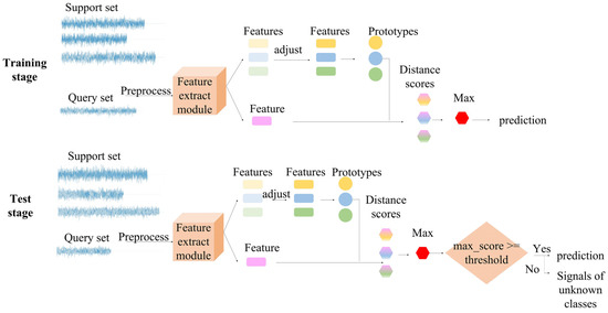
Figure 1. The overview of the IPN.

The main contributions can be summarized as follows:

• An approach based on PN belonging to meta-learning is proposed to realize few-shot signals recognition of known classes and signals distinguishment of unknown classes simultaneously for the first time in radar emitter signal recognition.
• RepVGG net is adopted instead of the original structure which limits the performance of the model seriously to increase the recognition performance.
• The way of obtaining prototypes in IPN is designed to avoid extreme samples affecting the prototypes by adding two trainable vectors to adjust the feature embedding vectors before average operation.
• The function of metric-based meta-learning that distinguishes samples of unknown classes is activated by setting a threshold in our method to verify whether samples belong to known classes or not.

This paper is organized as follows. Section 2 reviews some related works. In Section 3, the proposed IPN is introduced in detail. Section 4 presents our experiments and results. Section 5 is the discussion of the results. Section 6 gives a conclusion for this article.

2. Related Work

2.1. Radar Emitter Signal Recognition

Radar emitter signal recognition, which aims to obtain information about radar systems by analyzing the signals, is a key part of the electronic war and has been widely investigated by various researchers. Recent advanced achievements mainly rely on deep CNNs. Z. Liu designed a deep CNN with the input of time-frequency spectrums of radar signals in [13] to replace the manually designed features, which are time-consuming and ignore subtle characteristics. In [14], Y. Pan processed data with Hilbert–Huang transform to get abundant information about nonlinear and non-stationary characteristics of signals for identifying emitters and constructed a deep residual network to overcome the degradation problem, which improves efficiency. A novel one-dimensional CNN with an attention mechanism (CNN-1D-AM) was proposed by B. Wu in [15], which is time-saving in the data preprocessing stage by utilizing frequency signals. Additionally, relying on the attention mechanism to pay more attention to the key parts, the model achieves higher accuracy and superior performance on radar emitter signal recognition. Yuan. S constructed a 1-D selective kernel CNN (1D- SKCNN) for the classification of radar emitter signals in [16], which employed a multi-branch CNN and a dynamic selection mechanism in CNNs to allow each neuron to adaptively select its receptive field size based on multiple scales of input information. Considering that an emitter’s in-phase/quadrature (IQ) parameters will not change as it changes modulation schemes, Wong. L presented an approach in [17] for identifying emitters by using CNNs to estimate the IQ imbalance parameters of each emitter, which only used the received raw IQ data as input. To make full use of the received signals, pulse features, and time-frequency images of narrowband radar signals are utilized to be the inputs in [18], and Nguyen designed a model consisting of two parallel sub neural networks to process the two kinds of inputs. Similarly, to obtain more details of radar signals, a joint feature map that combines time-frequency and the instantaneous image was used in [19] as the inputs of a deep CNN. G. Shao proposed a deep fusion method based on CNNs in [20], which provides competitive results in terms of classification accuracy. In [21] Qu trained a CNN model and deep Q-learning networks, with the time-frequency images as the input extracted by Cohen class time-frequency distribution.

Among the methods of radar emitter signal recognition with deep learning, works are mainly done in two aspects to increase the recognition rates: one is the input of the networks, such as time-frequency images [13,21], signals on the field of frequency [15,16], other process methods of data [14,17], or mixture inputs [18,19], whose aim is to send more information about signals into models to improve the effects; the other aspect is the architectures of models, which is more important. For example, deepening or widening CNNs [13,14,20], or adopting some tricks [15,16] to improve the performance of models. The mentioned methods have achieved great performances in the field of radar emitter signal identification; however, deep learning-based radar emitter signal recognition methods require many labeled signals, which is difficult for some classes in the complex electromagnetic environment today. To solve this problem, we focus on few-shot radar emitter recognition in this article and propose a novel IPN method, which can achieve good performance based on a few labeled data.

2.2. Few-Shot Learning

Few-shot learning, which aims at recognizing novel categories from very limited labeled samples, is currently one of the most popular topics in the machine learning community. At present, there are three solutions to few-shot recognition: data augmentation, transfer learning, and meta-learning.

Data augmentation can alleviate the overfitting problem caused by a small number of labeled samples by expanding the amount of data. For instance, in [22], J. Ding utilized CNNs with domain-specific data augmentation operations to achieve synthetic aperture radar (SAR) target recognition. The method processes data with synthesis, translation, and adding noise, whose aim is to expand the data first, and then train the model as usual to realize the recognition of target samples directly. In transfer learning, target data is used to fine-tune a pre-trained model obtained from the source data instead of training a model directly, in order to relieve the problem of a small number of samples. To solve the problems of low probability of intercept radar waveform recognition rate and difficult feature extraction, Q. Guo presented an automatic classification and recognition system in [23] based on depth CNNs. To solve the problem of few samples, the method in [23] used a pre-trained feature extractor that comes from ImageNet trained models (interception-v3 and ResNet-152) combined with a classifier, in this way the model can converge easily even with few samples. In [24], Y. Peng introduced co-clustering to reconstruct source radar emitter signals to make them more related to target radar emitter signals, keeping the distribution similar, under which conditions the model can better adapt to target data. Then, with the utilization of transfer learning, it realizes the recognition of target data. A discriminant joint distribution adaptation algorithm is proposed by X. Ran in [25] to reduce the distribution discrepancy between the radar signals in the source domain and the target domain before transfer learning. With this method, the accuracy of recognition in the target domain is improved obviously. Aiming to realize few-shot SAR ship detection, Y. Li proposed a transfer learning-based deep ResNet to improve recognition accuracy in [26]. R. Shang proposed a deep memory CNN and a training strategy of the two-step transfer parameter technique in [27] to overcome the problem of overfitting caused by insufficient SAR image samples.

Meta-learning utilizes source data to enable models to obtain prior knowledge as well as transfer learning, while the training method is task-based in meta-learning which is different from data-based in transfer learning. Applications of meta-learning on few-shot recognition in other fields are sparse except in the field of image recognition. Methods in [6,7,8] are three classic metric-based meta-learning methods. Vinyals proposed matching networks (MN) in [6] to recognize query sets with cosine similarity. The PN in [7] is based on the basic hypothesis that there exists a class representation called prototype representation for each class. It realized few-shot recognition by comparing the Euclidean distance between prototypes and features of samples to the identification. F. Pahde designed a cross-modal feature generation framework [28] that can enrich the low populated embedding space in few-shot scenarios, leveraging data from the auxiliary modality. This method allows exploiting the true visional prototype and the prototype from additional modalities to compute a joint prototype which is more reliable. In [8], F. Sung presented to utilize CNNs instead with a fixed calculation method as the metric module to measure the relationship between a support set and a query set better. Based on the method of [7], S. Fort proposed Gaussian prototypical networks in [9], which estimate the confidence of individual points by the learned covariance maps, being able to learn a richer metric space. In [10], X. Zhang improved the model in [8] with multiple relation modules to get a much deeper relationship between the support set and query set. Recently, Lm proposed a novel contrastive learning scheme in [29] by including the labels in the same embedding space as the features and performing the distance comparison between features and labels in this shared embedding space with a novel loss function. This method is valuable and can be used for reference in metric-based meta-learning. A method called MAML is proposed in [4] with the aim of fast adaptation of deep networks. In this method, the networks will converge easier in fine-tuning stage at a good initialization obtained during the training stage. Additionally, in [11], N. Yang applied the method of [4] to radar emitter signal recognition for the first time in the field of radar emitter signal recognition successfully and obtained a good result. Y. Chen proposed a method that used neural networks to replace the gradient drop process in [5], achieving the aim of rapid adaptation with which the neural networks update the gradient more rapidly and accurately.

The networks will still be overfitted if the samples are too few even if transfer learning or data augmentation technology is utilized. In contrast, the meta-learning technique extracts transferable task agnostic knowledge from historical tasks and benefits from sparse data learning of specific new target tasks. Meta-learning makes it possible for models to obtain an ability learning to learn from the training strategy of meta-learning, which makes it much closer to artificial intelligence. Considering metric learning possesses an ability to distinguish signals of unknown classes by simply setting a threshold, and to make up for the vacancy in the application of meta-learning in radar emitter signal recognition, our method called IPN belonging to metric-based meta-learning is proposed with the reference to the development of metric-based meta-learning [6,7,8,9,10] in the field of image recognition.

Differently from the existing networks, our model not only utilizes the function of meta-learning that enables few-shot recognition but also pays attention to the function of metric learning, realizing signals distinguishment of unknown classes by setting a threshold. In consequence, two problems mentioned in the abstract can be solved with this method.

3. Methods

3.1. Task Description

Meta-learning aims to enable a model to possess an ability to learn from the training stage with the tasks sampled from the source data, as a result, the model with this ability can realize few-shot recognition on the target data successfully. In the few-shot radar emitter recognition problem, the target data refers to some classes which we want to identify but with only a few labeled signals, and the source data refers to classes of radar signals with a large number of samples. With the application of meta-learning in radar emitter signal recognition, we want to train the model in a task space based on the source data to obtain meta-knowledge, in consequence, few-shot recognition in the field of radar emitter signal identification is achieved. The formulation of datasets and tasks are described in the following.

In meta-learning, there is a training set, a validation set, and a test set with a number of classes, and each class contains multiple samples.

In the training stage, an N-way K-shot meta task is constructed by randomly selecting N classes from the training set and K samples in each selected class (totally N × K samples, K is a small number), which is called a support set. Then, a batch sample will be extracted from the remaining data in the selected classes as a query set belonging to the support set. During the training process, the recognition ability is learned by sending a number of different meta-tasks into the model.

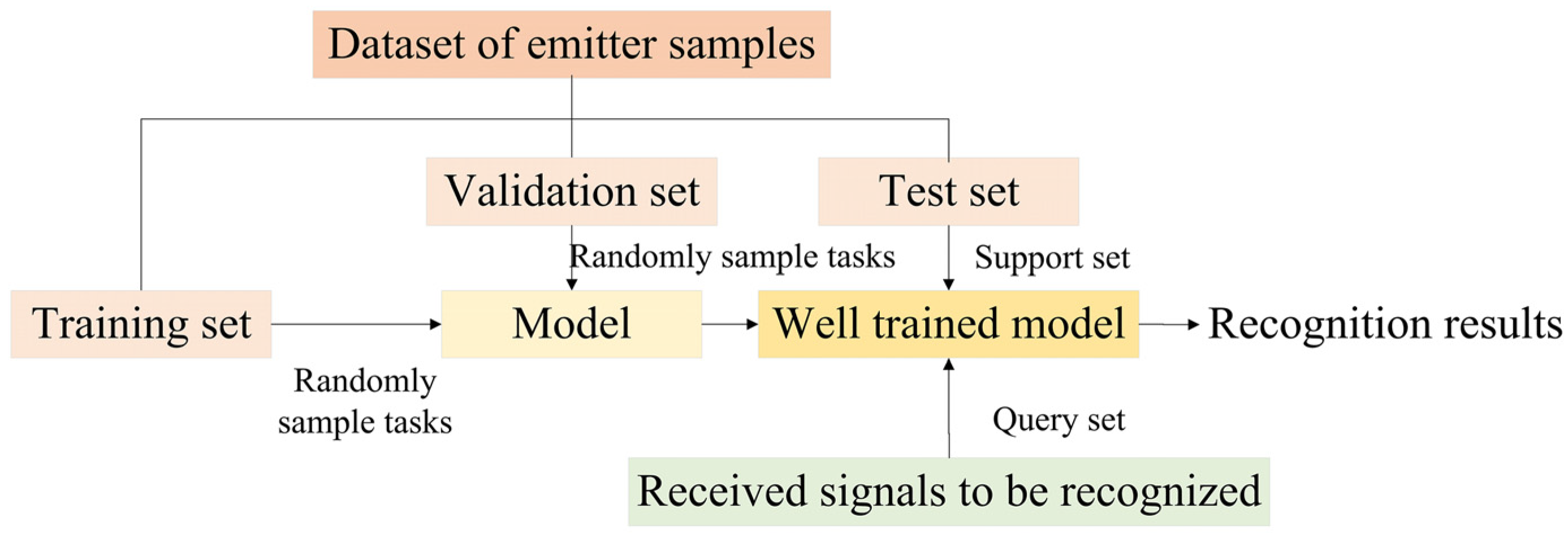
To apply meta-learning to radar emitter signal recognition, the datasets in the field are built in the same way, as shown in Figure 2. There is a training set with X classes, a validation set including Y classes that are different from those in the training set, and a test set including N classes that differ from the above. The formulation of the dataset can be understood in this way: there is a dataset including radar signals of X + Y + N classes, and each class in (X + Y) contains multiple samples, each class in N classes contains a few samples that are larger than K, which refers to some kinds of radar signals that only have a few samples. We want to realize signals recognition of these N classes with the help of signals in (X + Y) classes. We divided the (X + Y) classes into a training set used to train a model, and a validation set used to examine whether the model performs well on unseen classes for few-shot recognition. N-way K-shot tasks are sampled from the training set during the training stage to enable the model to obtain meta-knowledge. When the well-performed model is chosen, we apply the model to recognize signals of the N classes. During this test stage, the support set is sampled from the few samples in the N classes in the test set, and the query set includes signals to recognize in these N classes we received in the future. The process in a real scene is shown in Figure 3.

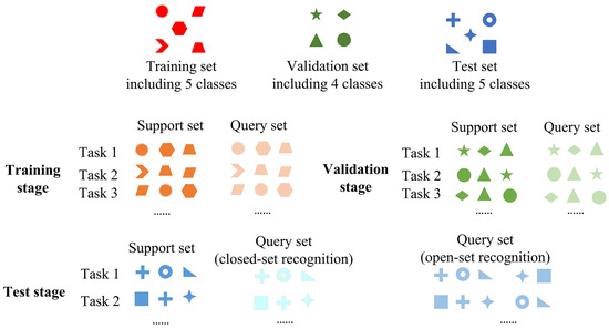
Figure 2. The formulation of the training set, validation set, and test set, and the method of obtaining tasks. There is an example under the condition as follows: the training set includes 5 types of samples, the validation set includes 4 types of samples, the test set includes 5 types of samples, and 3-way 1-shot tasks are randomly sampled, that is, X = 5, Y = 4, Z = 5, N = 3, K = J = 1.

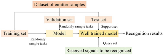
Figure 3. The process of realizing few-shot radar emitter signal recognition.

However, in our experiments, the test set includes Z (Z > N) classes and each class contains the number of samples in order to test the performance of the final model. Each task in the test stage is a simulation of few-shot radar emitter signal recognition, and we sample a recognition task like this: firstly, N classes are randomly sampled; and then K samples in these classes are randomly chosen to be regarded as few samples we owned in these classes; after that, another J samples in the N classes are chosen to be regarded as the signals to recognize; the (N + K + J) samples consist of a recognition task.

When it comes to open-set recognition, that is, few-shot signal recognition of known classes and distinguishment of signals of unknown classes, the formulation is completely the same as what is described above, except for the test stage. In each epoch of the test stage, another J samples in the classes left are randomly chosen to be regarded as the signals of unknown classes to distinguish.

3.2. Improved Prototypical Network

Few-shot recognition based on meta-learning is mainly applied in the image recognition field, and metric-based meta-learning is a kind of method of meta-learning. As a result of images’ 2-dimensional attributes and characters, the networks of metric-based meta-learning in the image field adopt 2D-CNNs and a small size max pool. While in radar emitter signal recognition, signals we received are 1D time signals, although the networks in the image field can be used directly with the operation of changing 1D time signals to time-frequency spectrum, time-frequency transformation is time-consuming, enlarging the work of preprocessing and lowing the speed of recognition. In fact, the frequency characteristics of radar signals are obvious enough to distinguish most types of radar signals. Moreover, the preprocessing speed of the fast Fourier transform (FFT) is much faster than that of the time-frequency transform, and 1D CNNs based on frequency signals reduce many parameters compared to 2D CNNs based on time-frequency spectrums. In summary, the 1D recognition networks have more advantages than the 2D recognition networks in the field of radar emitter recognition. As a consequence, we apply the metric-based meta-learning method to few-shot radar emitter signal recognition with 1D CNNs.

In addition, metric-based meta-learning in the image field only utilizes the characteristic of meta-learning to realize few-shot recognition of known classes, while the function that metric networks own of distinguishing samples of unknown classes is ignored. In radar emitter signal recognition, research is sparse on open-set signal recognition. However, signals we received to recognize can not only contain signals of known classes in practical application, but there must be some signals of unknown classes, and without interference, the recognition networks will classify these signals of unknown classes to one of the known classes compulsively, affecting the subsequent analysis of radar systems. Whether the networks could realize open-set recognition is one of the problems in radar emitter signal recognition. Therefore, in our method, the function of metric learning is utilized to realize open-set recognition with a settled threshold.

The IPN we proposed consists of three modules: a feature extracting module, a prototypical module, and a metric module. Differing from PN, we add two trainable vectors to learn a suitable adjustment for feature vectors of the support set, which aims to obtain a more reasonable prototype representation and to prevent some extreme samples from affecting the prototype location seriously. In addition, we adopt a RepVGG net instead of the original VGG net, that is, during the training process, we use a multi-branch network structure to improve model performance, and during the test process, we transform it to a single branch network structure to avoid occupying too much memory and slowing the calculation speed. Moreover, we utilize 1D CNNs in the feature extracting module to suit radar signals perfectly and avoid complex data pretreatment which is time-consuming.

The data processing flow is shown in Figure 4: the feature extracting module $f_{\varphi }$ extracts feature vectors of support samples and query samples. After that, in the prototypical module, the K support samples’ feature vectors are multiplied by a trainable vector $\gamma$ and then plus a trainable vector $\beta$ to reduce the influence on the prototype, and then N prototypes are obtained by averaging the adjusted support feature vectors in the same classes. Finally, the metric module calculates the distance scores and makes predictions by comparing the distance scores between each query sample and each prototype. More details of our network are described in the following sections.

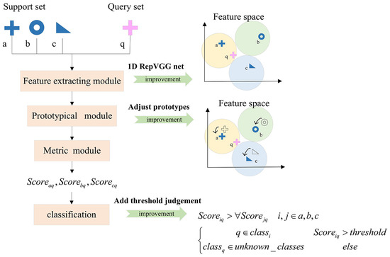
Figure 4. Processing flow and improvements.

3.2.1. Feature Extracting Module

The feature extracting module is used to extract a feature vector from each signal input. In [7], this module is just four CNN blocks stacked and the numbers of convolutional kernels per block are 64, 64, 64, and 64.

The numbers of convolutional kernels per block are 64, 64, 64, and 64.

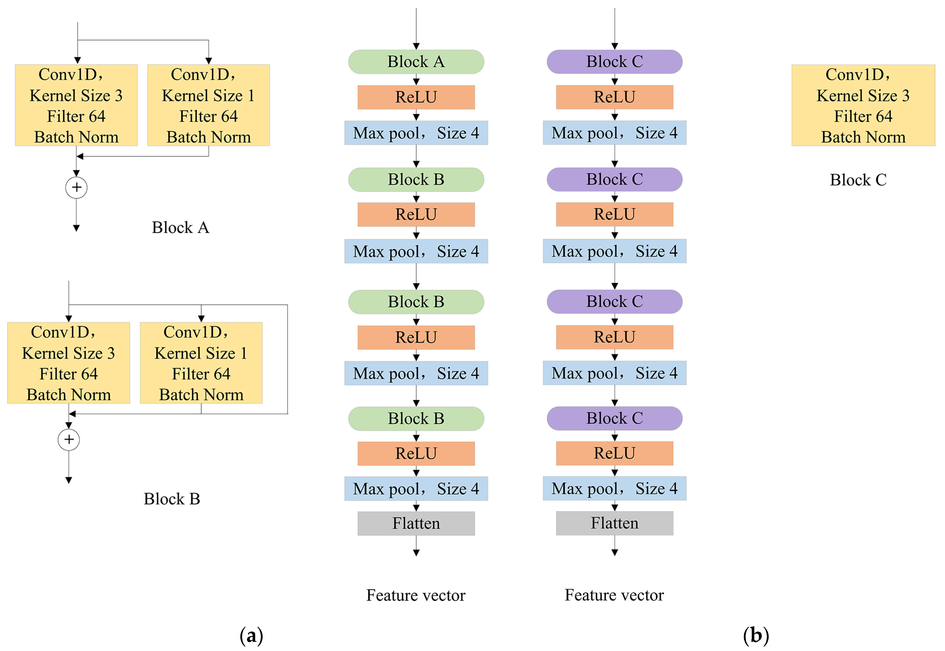
Considering that such a simple CNN structure is not able to extract feature vectors for complex data well, we use RepVGG net to take the place of the feature extracting net in [7]. As shown in Figure 5, we still use four CNN blocks, but add one or two branches to each block to increase the performance of the model. Through the method of architecture re-parameterization in [12], we decouple the training-time multi-branch and inference-time plain architecture, taking into account the performance in the training process and the running speed in the test process. Moreover, we not only choose 1-D CNN instead, but also change the size of the max pool to 4, as the reason that the length of received radar signals is much larger than images, and enlarging the max pool size will reduce the parameters which are beneficial to avoid overfitting and accelerate the training process.

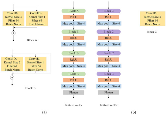
Figure 5. (a) Training architecture shows the structure in the training process, which includes two or three branches to improve performance; (b) Inference architecture is the structure in the test process, which is transformed from multi-branch by architecture re-parameterization.

3.2.2. Prototypical Module

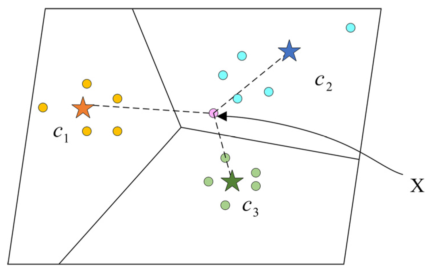
This module aims to generate a prototype for each class in the support set. In [7], they define a class’s prototype as the mean of its support feature vectors, which can be affected easily. Because the problem we face is few-shot recognition, it means that in some classes we may only have 5 samples or even 1 sample. We tend to want the prototype to be located at the position where most feature vectors of samples gather; however, one special sample can pull the prototype far from where more samples gather because the samples are few. This is illustrated in Figure 6.

Figure 6. The query sample X belongs to class $c_2$, while its distance with class $c_3$ is shorter.

The deviation of prototypes will directly affect the judgment of which class query samples belong to. In order to reduce the influence, we introduce two trainable vectors $\gamma$ and $\beta$ to adjust support feature vectors before the average operation.

We define the support set to include N classes and each class contains K samples of D dimension. Each sample is mapped into the M-dimensional feature space by the feature extracting module $f_{\varphi }$, where $\varphi$ refers to the learnable parameters of the feature extracting network. Then the process of obtaining prototypes is as follows:

$$c_n=\frac{1}{K}{\displaystyle \sum _{(x_i,y_i)\in S_n}\gamma f_{\varphi }(x_i)}+\beta$$

(1)

where $c_n$ is the prototype of class $n$, $(x_i,y_i)\in S_n$ means the samples belong to class $n$ in this support set and $y_i$ is the label of the radar sample $x_i$, $f_{\varphi }(x_i)$ represents the M-dimensional feature vector of $x_i$, and $\gamma$ and $\beta$ are our scale and shift vectors both with M dimension.

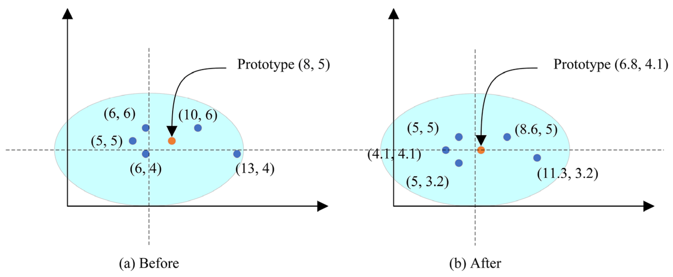
We hope the two vectors can learn how to adjust the prototypes through the training stage. Figure 7 explains how the two vectors work.

Figure 7. Take the 5-shot problem and 2-dimensional feature vector as an example. The left figure shows the prototype provided by average operation only, where there is a deviation on the prototype. In this example, simply assuming our $\gamma$ is (0.9, 0.9) and $\beta$ is (−0.4, −0.4), feature vectors are dealt with the scale and shift vectors in front of averaging, and the right figure is achieved. It is obvious that the prototype of the right figure is much closer to the center than that of the left figure.

3.2.3. Metric Module

The metric module is to estimate the distance score between a feature vector of a query signal and a class prototype representation. The loss function we use is replaced by mean square error (MSE).

Firstly, we calculate the distance score with input prototypes and query feature vectors.

$$\begin{array}{l}{d}_{iq}={\Vert f_{\varphi }(x_q)-c_n\Vert }_2\\ scor{e}_{iq}=e^{-d_{iq}}\end{array}$$

(2)

where $d_{iq}$ is the Euclidean distance between $c_i$, the prototype of class $i$, and the feature vector $f_{\varphi }(x_q)$ of the query sample $x_q$; $scor{e}_{iq}$ is the distance score.

When it comes to the test of signal recognition including unknown classes, a threshold judgment is added to identify whether signals belong to known classes.

$$\begin{array}{l}\begin{array}{cc}scor{e}_{iq}>=\forall scor{e}_{jq}& i,j\in \left\{0,1,\cdot \cdot \cdot ,N\right\},q\in \left\{0,1,\cdot \cdot \cdot ,J\right\}\end{array}\\ \{\begin{array}{cc}{x}_q\in clas{s}_i& scor{e}_{iq}>threshold\\ x_q\in unknown\_classes& else\end{array}\end{array}$$

(3)

The objective function is as follows:

$$\begin{array}{l}J(\varphi ,\gamma ,\beta )={\displaystyle \sum _{l=1}^L{(scor{e}_l-t_{n,j})}^2}\\ t_{n,j}=\{\begin{array}{cc}1& y_n=y_j\\ 0& else\end{array}\end{array}$$

(4)

Learning proceeds by minimizing $J(\varphi ,\gamma ,\beta )$ via stochastic gradient descent (SGD). The pseudocode to compute the loss for a training episode is provided in Algorithm 1.

Algorithm 1: Episode-based training for IPN

Input: the training set

$\hspace{1em}\hspace{1em}\mathrm{Initialization}: \mathrm{Randomly} \mathrm{initialize} \mathrm{model} \mathrm{parameters} \varphi ,\gamma ,\beta$, and learning rate α

For i = 1: episode number

$\hspace{1em}\hspace{1em}\hspace{1em}\hspace{1em}{V}_n$ Randomly sample N classes from the training dataset

$\hspace{1em}\hspace{1em}\hspace{1em}\hspace{1em}S={\{(x_k,y_k)\}}_{k=1}^K$ Randomly extract K samples from each of the N classes

$\hspace{1em}\hspace{1em}\hspace{1em}\hspace{1em}Q={\{(x_j,y_j)\}}_{j=1}^J$$\mathrm{Randomly} \mathrm{extract} \mathrm{J} \mathrm{samples} \mathrm{from} V_n/S$

$\hspace{1em}\hspace{1em}\hspace{1em}\hspace{1em}\mathrm{While} J(\varphi ,\gamma ,\beta )>\epsilon$

$\hspace{1em}\hspace{1em}\hspace{1em}\hspace{1em}\hspace{1em}\hspace{1em}\mathrm{Update} \varphi ,\gamma ,\beta \leftarrow \varphi ,\gamma ,\beta -\alpha {\nabla }_{\varphi ,\gamma ,\beta }J(\varphi ,\gamma ,\beta )$

End while

Output: Model parameters ϕ, γ, β

4. Experiments

In this section, we evaluate our approach to radar emitter recognition. We first produced a radar emitter signal dataset, and divide it into a training set, a validation set, and a test set as described in Section 3. Then with the use of the training set and the validation set, we trained the networks proposed in Section 3. Finally, we applied the well-trained networks on the test set to achieve few-shot radar emitter recognition and unknown signal distinguishment by setting a threshold. If the highest score is lower than the threshold, the query signal will be considered as a signal of an unknown class, if not, the type of the highest score is the prediction result.

4.1. Dataset

Fourteen different varieties of radar emitter signals were used to evaluate the effectiveness of the proposed method, which includes continuous (CW), linear frequency wave (LFM), nonlinear frequency wave (NLFM), binary phase-shift keying (BPSK), quadrature phase-shift keying (QPSK), binary frequency shift keying (BFSK), quadrature frequency shift keying (QFSK), multi-component linear frequency wave (MLFM), double linear frequency wave (DLFM), even secondary square linear frequency wave (EQFM), and mixed modulation BPSK-LFM, BFSK-BPSK, BFSK-QPSK, QFSK-BPSK. These 14 different emitter signals [15,16] are commonly used in radar systems. The specific parameters of the signals are shown in Table 1.

Table 1. Specific parameters of the 14 radar emitter signals.

	Signal Type	Carrier Frequency	Parameter
Emitter 1	CW	200~250 MHz	None
Emitter 2	LFM	200~250 MHz	Frequency bandwidth: 30–32 MHz
Emitter 3	NLFM	200~250 MHz	Frequency of modulation signal ranges from 10 to 11 MHz
Emitter 4	MLFM	100~120 MHz 140~160 MHz	Frequency bandwidth: 30–32 MHz
Emitter 5	DLFM	200~250 MHz	Frequency bandwidth: 30–32 MHz
Emitter 6	EQFM	200~250 MHz	Frequency bandwidth: 30–32 MHz
Emitter 7	BPSK	200~250 MHz	13-bit Barker code
Emitter 8	BFSK	100~120 MHz 140~160 MHz	13-bit Barker code
Emitter 9	QPSK	200~250 MHz	16-bit Frank code
Emitter 10	QFSK	100~120 MHz 140~160 MHz 180~200 MHz 220~240 MHz	16-bit Frank code
Emitter 11	BPSK-LFM	200~250 MHz	Frequency bandwidth: 30–32 MHz 13-bit Barker code
Emitter 12	BFSK-BPSK	100~120 MHz 140~160 MHz	13-bit Barker code
Emitter 13	BFSK-QPSK	100~120 MHz 140~160 MHz	16-bit Frank code
Emitter 14	QFSK-BPSK	100~120 MHz 140~160 MHz 180~200 MHz 220~240 MHz	16-bit Frank code 13-bit Barker code

Note 1: The pulse width for each signal ranges from 1 to 2 us; Note 2: Sampling frequency is 1 GHz.

The dataset how we produced is described as follows:

(1)

First, we generated 14 types of radar emitter signals with different values of SNR. The SNR for each type of signal ranged from 0 to 9 dB with 1 dB step, containing a total of 10 values. The number of samples for each type of signal with each value SNR was 200;

(2)

Second, we utilized 2000 points FFT to process signals processed in (1). To ensure different data samples under the same distribution scale, z-score standardization is adopted to process input data, which is also beneficial to network optimization and training-time reduction. Assuming the sample sequence of a radar emitter signal is $x=[x_1,\cdot \cdot \cdot ,x_U]$, where U is the number of sample points. The value of each point of this sequence after standardizing is detailed below:

$$x_u^{\prime }=(x_u-\overline{x})/s$$

(5)

where $\overline{x}$ is the mean of radar emitter sequence, and $s$ is the standard deviation:

$$\begin{array}{l}\overline{x}=\frac{1}{Z}{\displaystyle \sum _{z=1}^Z{x}_z}\\ s=(\frac{1}{Z-1}{\displaystyle \sum _{z=1}^Z{(x_z-\overline{x})}^2}{)}^{1/2}\end{array}$$

(6)

(3)

Third, we divided the dataset into a training set, a validation set, and a test set as described in Section 3.1. In order to avoid the accident caused by different ways of dividing the dataset, three experiments were done to examine the networks’ performance. The different classifications of the dataset in experiments are described in Table 2.

Table 2. Different classifications of experiments.

	Dataset 1	Dataset 2	Dataset 3
Training set (5 types)	CW, LFM, NLFM, MLFM, EQFM	CW, BPSK, BFSK, QPSK, BFSK-QPSK	BPSK, QPSK, QFSK, BFSK-BPSK, QFSK-BPSK
Validation set (4 types)	BPSK, BFSK, QPSK, QFSK	NLFM, MLFM, BPSK-LFM, QFSK-BPSK	LFM, DLFM, EQFM, BFSK-QPSK
Test set (5 types)	DLFM, BPSK-LFM, BFSK-BPSK, BFSK-QPSK, QFSK-BPSK	LFM, EQFM, DLFM, QFSK, BFSK-BPSK	CW, NLFM, MLFM, BFSK, BPSK-LFM

4.2. Results

In order to show the superiority of the proposed method, in this section, we will compare the proposed method with the application of MAML on radar emitter signal recognition [11], and other approaches of metric-based meta-learning, including MN [6], PN [7], and relation network (RN) [8].

We simulated 3-way 5-shot and 3-way 1-shot closed-set recognition in three datasets as described in Section 4.1 to avoid contingency, and query samples used are five per class. In the experiments, the settings of [6,7,8] are the same as those in the references except the CNN we used is 1D, and the setting of [11] is completely the same as what is described in [11]. At the stage of training, the optimization algorithm for the proposed IPN is adaptive moment estimation (ADAM). The batch size of tasks is 32 and we have run 100 epochs for training, where the learning rate is 0.0005. The weights used for the test stage are saved when the accuracy of the validation set is highest.

We did two types of examination during test time as said in Section 3.1. One type of examination is to see the performance of models under the condition that recognition signals all belong to known classes, that is, a test of closed-set recognition. The other type of examination is to see the performance of models under the condition that there are signals out of known classes, which is a test of open-set recognition. The test accuracy is the average accuracy of 20,000 tasks randomly sampled in the test set. Table 3 shows closed-set few-shot recognition.

Table 3. Classification accuracies on closed-set few-shot recognition.

	Model	3-Way 1-Shot	3-Way 5-Shot
Experiment 1	MAML [11]	81.045%	92.233%
	MN [6]	81.331%	81.842%
	RN [8]	89.885%	92. 652%
	PN [7]	88.826%	94.232%
	OURS	91.827%	95.157%
Experiment 2	MAML [11]	78.769%	92.581%
	MN [6]	79.876%	79.825%
	RN [8]	85.020%	87.111%
	PN [7]	90.724%	95.727%
	OURS	96.568%	98.178%
Experiment 3	MAML [11]	91.238%	97.528%
	MN [6]	87.835%	88.005%
	RN [8]	87.146%	85.682%
	PN [7]	99.397%	99.919%
	OURS	99.997%	100%

Note: The datasets used in experiment 1, experiment 2, and experiment 3 are dataset 1, dataset 2, and dataset 3 respectively.

It is indicated that the accuracy of the 5-shot is higher than that of the 1-shot evidently for any model in the experiments, as the consequence of a large support set is conducive to the construction of a detailed description of the classification task, which is beneficial to the model to learn generalized characteristics in the training stage. Besides, it can be observed that our IPN achieves the best performance in all three experiments on the few-shot recognition of radar emitter signal recognition. We gain a good result for the 5-shot classification. Comparing to the application of MAML on radar emitter signal recognition [11], we get higher accuracy of about 98.178% in experiment 2, which is about 6 percentage points higher than that of the method in [11]. What is more, we receive an average accuracy of 96.568% of IPN in the 3-way 1-shot in experiment 2, which shows our method achieves nearly six percentage points improvement to PN, proving that IPN is more effective than the original PN. This is partly because we add two vectors to adjust the prototypes. As a result of the prototype idea being based on the thought that the abstract representation vector of the class, a support vector set is used to classify the query vector instead of the original support vectors. This improvement is very helpful for avoiding the misclassification caused by the metric based on the support vectors in the case of limited labeled samples. We add an adjustment operation before averaging, fully considering the influence of extreme samples, and get a prototype expression that is better than averaging directly. In addition, our improvement on the feature extracting module also contributes to the increase in accuracy. This improvement develops the ability to extract characteristics of the network, which is beneficial to the model to adapt to radar emitter signals.

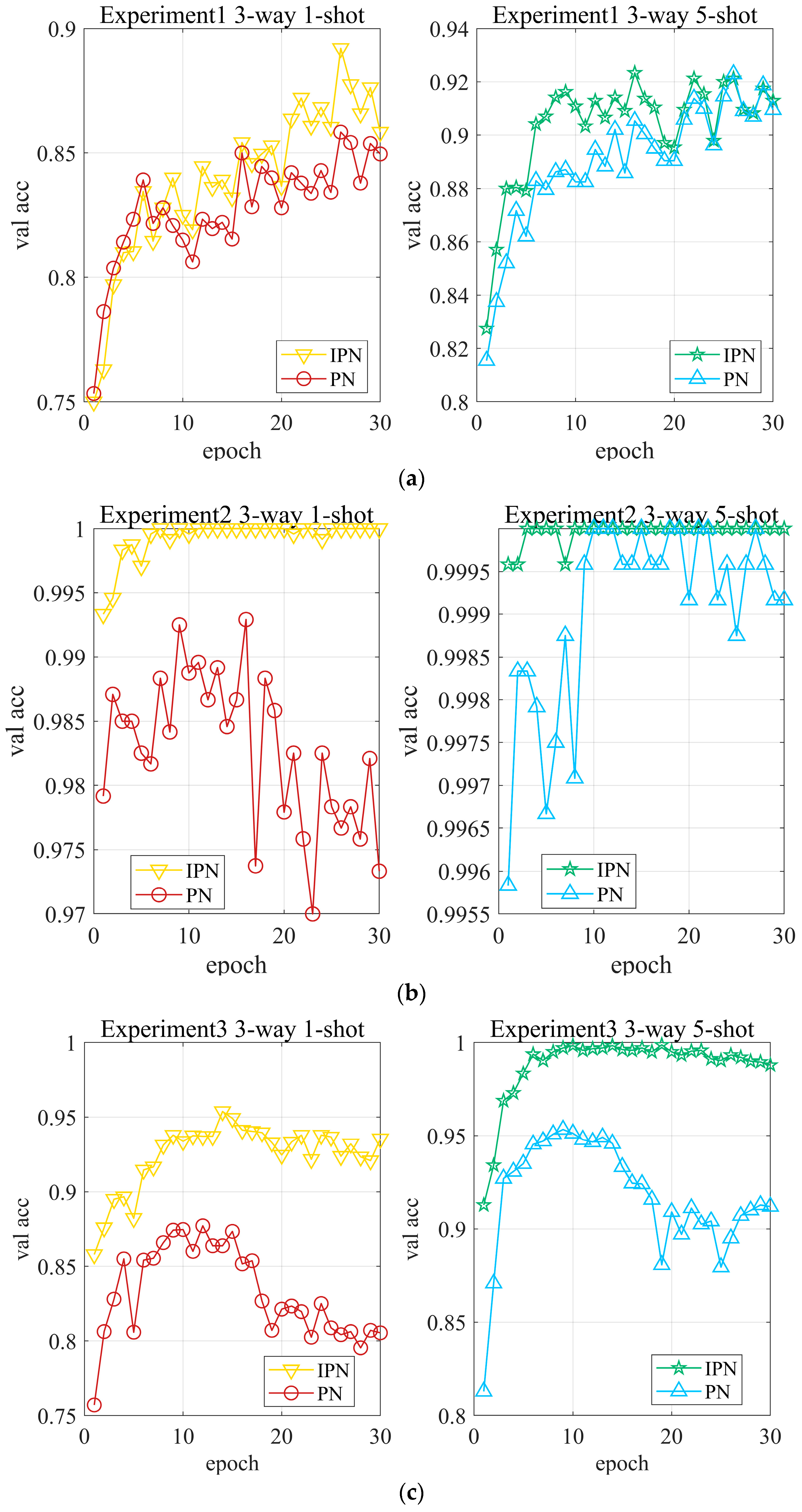
The validation accuracies of PN and IPN during the training stage are described in Figure 8. By analysis, the accuracy of IPN is mostly always higher than that of PN, and the performance of IPN is much superior to that of PN. Besides, it can be seen from the figure that our method reaches the optimal point faster and has better stability. Specifically, we can know from the 1-shot validation accuracies of experiment 1 that IPN and PN both get the best performance at the epoch of 26, while the accuracy of IPN is obviously higher than that of PN. Additionally, by observing 1-shot validation accuracies of experiment 2, it is found that IPN reaches the optimal point and the accuracy curve tends to be stable, and comparing the accuracy curve of PN, which is still shaking, our model has better stability. What is more, it is shown in the 1-shot accuracies of experiment 3 that after an epoch of training, the accuracy of our method is nearly 85%, which is about 10 percentage points higher than that of PN, which proves the superior performance of our model.

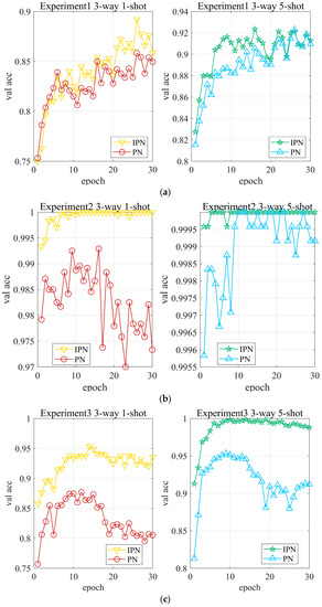
Figure 8. Validation accuracies of PN and IPN in experiments. (a) Experiment 1, (b) Experiment 2, (c) Experiment 3.

Table 4 shows the performance of open-set recognition of IPN and PN, that is, the performance of realizing both few-shot recognition of known classes and the distinguishment of unknown classes. Acc1 refers to the accuracy of few-shot recognition of known classes and the distinguishment of unknown classes at the same time, and Acc2 refers to the accuracy in distinguishing known classes and unknown classes.

Table 4. Classification accuracies on few-shot recognition of known classes and distinguishment of unknown classes at the same time.

	Model	3-Way 1-Shot		3-Way 5-Shot
		Acc1 *	Acc2	Acc1	Acc2
Experiment 1	PN [7]	65.231%	71.437%	78.278%	80.840%
	OURS	75.325%	79.564%	81.795%	84.671%
Experiment 2	PN [7]	73.655%	77.995%	81.279%	82.985%
	OURS	87.375%	88.123%	87.509%	88.085%
Experiment 3	PN [7]	76.014%	76.258%	83.144%	83.178%
	OURS	81.717%	81.717%	87.754%	87.754%

* Note: Acc1 refers to the accuracies in few-shot recognition of known classes and distinguishment of unknown classes at the same time and Acc2 refers to the accuracies in distinguishing known classes and unknown classes only.

It can be seen from Table 4 that the recognition accuracies of our method are always higher than those of PNN in the three experiments. Acc2 of IPN in 1-shot recognition of experiment 2 has nearly 11% improvement compared to that of PN, which shows our model has a better performance in distinguishing signals of unknown classes. The reason is analyzed to see that our improvement on the feature extracting module shows its advantage. As the repVGG net is more complex than the original network, it can extract more information and abundant features of inputs. If the model receives signals of unknown classes, there will be obvious differences between the feature vectors of these signals and those of known classes, and so the model can distinguish whether signals belong to known classes or not with the help of the threshold.

To further show the advantages of our method, we recorded the time usage of the training stage and test stage, which can be seen in Table 5 and Table 6. The training time for an epoch of IPN is a bit more than that of PN, while the test time for 1000 tasks of IPN is smaller, which means our model can make predictions faster in practical application, contributing to speeding up our analysis of enemy radar systems. This is because we transform the model from multi-branch in the training stage to plain architecture in the test stage by architecture re-parameterization as described in Section 3.2.1. Our method reduces the inference time in the test stage and increases the closed-set recognition accuracy by 1 to 6 percentage points and open-set recognition accuracy by 4 to 10 percentage points.

Table 5. The time usage of the methods to preprocess 1 epoch in the training stage.

Model	3-Way 1-Shot	3-Way 5-Shot
PN [7]	22.160 s	33.963 s
OURS	33.309 s	53.063 s

Table 6. The time usage of the methods to preprocess 1000 recognition tasks in the test stage.

Model	3-Way 1-Shot	3-Way 5-Shot
PN [7]	23.000 s	31.408 s
OURS	14.018 s	19.787 s

5. Discussion

The prototype of each class is determined by samples in the support set, and the model is continuously optimized through the query set. Therefore, selecting different numbers of support set samples and the query set samples may have an impact on the training of the model. Besides, among methods of meta-learning, the task settings for training and testing should be the same. In other words, if we want to perform a 3-way 1-shot task, the same 3-way 1-shot setting should be maintained in the training stage. What if the conditions are mismatched? As a result, we investigate the influence of these factors on few-shot recognition in this section.

5.1. Influence of the Number of Support Samples on Recognition Accuracy

In the training stage, we fix the number of ways but vary the number of shots in the training stage to learn several different models. Then in the test stage, we test the five well-trained models under their corresponding shot settings. A 3-way K-shot (K = 1, 5, 10, 20, 40) task is conducted on dataset 1 by using PN and IPN.

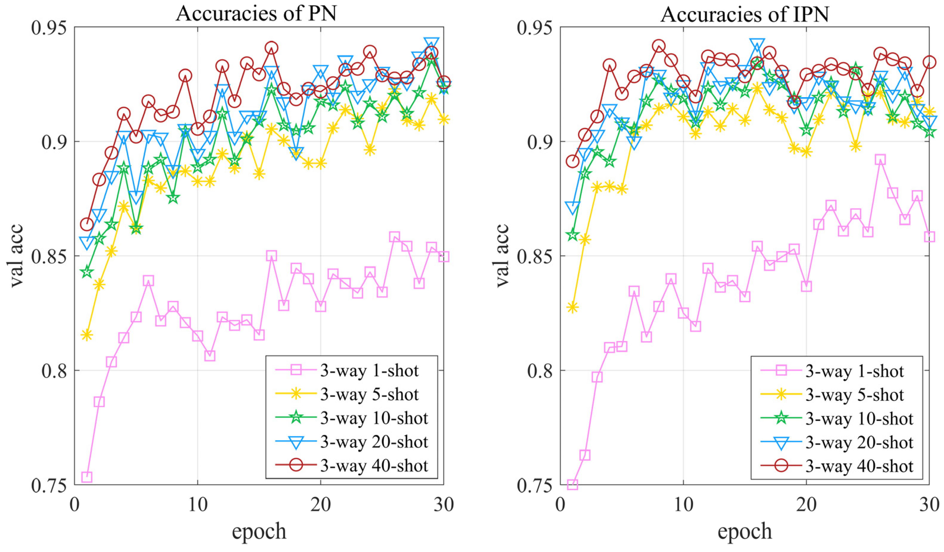
Figure 9 shows the validation accuracy of PN and IPN with different support set samples during the training stage. It is indicated that IPN with 1-shot, 5-shot, 10-shot, 20-shot, and 40-shot support set samples has reached the optimal points at epochs 25, 15, 15, 11, and 7 respectively. As a result, the validation accuracy of the model and the speed of reaching the optimal point become higher with the increase in the number of support set samples. However, this is not to say that the larger the number of support samples, the better the model, which can be seen in Table 7, showing the test accuracies of PN and IPN with different support set samples. With the increase in the number of support set samples, test accuracies rise sharply at first and then tend to be stable. In consequence, we can improve the model performance by increasing the number of support set samples, but it should be noted that the size of the support set is not supposed to be too large, which will increase the training cost and the benefit is low. Table 8 describes the open-set few-shot recognition of PN and IPN with different support set samples, where we can obtain the same conclusion as above. Moreover, it can also be seen in Table 7 and Table 8 that IPN’s recognition accuracies are always higher than PN’s recognition accuracies, showing the superiority of our method.

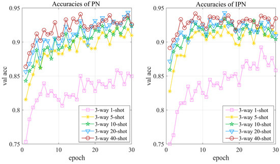
Figure 9. Validation accuracy of PN and IPN with different support set samples.

Table 7. Classification accuracy on closed-set few-shot recognition with different support set samples.

Model	3-Way 1-Shot	3-Way 5-Shot	3-Way 10-Shot	3-Way 20-Shot	3-Way 40-Shot
PN	88.826%	94.232%	94.824%	95.302%	95.248%
OURS	91.827%	95.157%	95.592%	95.771%	95.746%

Table 8. Classification accuracy on open-set few-shot recognition with different support set samples.

	Model	3-Way 1-Shot	3-Way 5-Shot	3-Way 10-Shot	3-Way 20-Shot	3-Way 40-Shot
Acc1	PN [7]	65.231%	78.278%	78.848%	77.830%	78.153%
	OURS	75.325%	81.795%	86.345%	86.571%	85.482%
Acc2	PN [7]	71.437%	80.840%	81.564%	80.457%	80.421%
	OURS	79.564%	84.671%	88.945%	89.045%	87.916%

5.2. Influence of Query Samples on Recognition Accuracy

To explore the influence of the number of query samples, 3-way 1-shot experiments on IPN with different query set samples are conducted with dataset 1. In the training stage, we fix the task by setting it as a 3-way 1-shot, but vary the number of the query set samples in each class. The validation accuracy is shown in Figure 10. By observing that the accuracy curves are almost the same, it is suggested that query set samples do little influence on the model performance.

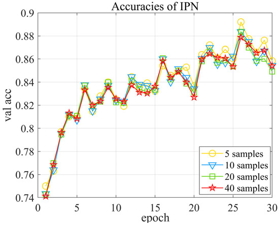
Figure 10. Validation accuracy of IPN with different query samples.

5.3. Influence of Mismatching Condition

In order to analyze the influence of mismatching conditions on recognition accuracy, we fix the number of ways but vary the number of shots in the training stage to learn several different models. Then in the test stage, we test the five well-trained models under different shot settings, where the number of shots is changed. A 3-way K-shot (K = 1, 5, 10, 20, 40) task is conducted on dataset 1 by using our IPN. The results are given in Table 9, where the entries on the diagonal are the results of the matching condition.

Table 9. Classification accuracies on closed-set few-shot recognition with different support set samples the 3-way K-shot mean accuracy of IPN by varying the number of shots (K = 1, 5, 10, 20, 40). For each test setting, the best result is highlighted.

Task Settings for the Train Stage	Task Settings for the Test Stage
	3-Way 1-Shot	3-Way 5-Shot	3-Way 10-Shot	3-Way 20-Shot	3-Way 40-Shot
3-Way 1-Shot	91.827%	94.956%	95.529%	95.702%	95.854%
3-Way 5-shot	92.299%	95.157%	95.618%	95.850%	95.968%
3-Way 10-shot	92.158%	95.101%	95.592%	95.840%	95.943%
3-Way 20-shot	92.059%	95.072%	95.564%	95.771%	95.932%
3-Way 40-shot	91.478%	94.785%	95.320%	95.593%	95.746%

We found that the 3-way 5-shot model has the best accuracy for any 3-way K-shot recognition in the test stage compared with other models. We infer the reason is that under the condition that the task setting is 1-shot in the training stage, the extracted features are limited by the sample size, leading to underfitting of the parameters; when it comes to the case that the number of samples per class is larger than 10, the parameters will be more suitable for the characteristics of the training set with the optimization of the model, lowing the generalization of the model. Five samples per class in the support set are appropriate for the learning of the parameters of IPN and the well-trained model has good generalization for any shot recognition tasks.

Considering the experiments we did in Section 5.1, the model trained with the setting of 3-way 10-shot has good accuracy for both open-set recognition and closed-set recognition, and we can find from Table 9 that the accuracy of the 3-way 10-shot model for 3-way K-shot recognition is excellent, although it is slightly lower than the 3-way 5-shot model, which is the best model. In summary, we consider the 3-way 10-shot as the best setting for IPN.

6. Conclusions

A novel metric-based meta-learning method IPN is proposed to solve open-set few-shot recognition in the field of radar emitter signal recognition. For the problem that the simple networks inadequately extract the abstraction features of samples, we utilize RepVGG net to improve extracting high-level feature vectors of the samples. To address the issue that prototypes are affected easily by some extreme samples, we introduce two trainable vectors to adjust the feature vectors of samples before the operation of averaging. Aiming at the situation that the research is few on open-set recognition in the field of radar emitter signal recognition, we set a threshold in the metric module to distinguish the signals unknown classes, realizing open-set recognition. The comparison results with other metric-based methods and the application of MAML on radar emitter signal recognition show the superior performance of IPN. From the further experiments of exploring the settings to improve the few-shot recognition accuracy of IPN, we suggest that the 3-way 10-shot may be the best setting for our model to realize open-set few-shot recognition on radar emitter signals for any 3-way K-shot test. We also realize the shortcomings of our method. As a consequence of the threshold being artificially set according to the model’s performance on the validation set, there are two problems: first, the threshold setting is subject to a certain degree of subjectivity; secondly, there is a difference in data distribution between the validation set and the test set, that is, the threshold which is set according to the validation set may not be perfectly applicable to the test set. In future work, we hope to develop a method to realize threshold adaptive setting and explore an approach to reduce the difference in data distribution between the validation set and the test set.

References

- Schmidhuber, J. Deep Learning in Neural Networks: An Overview. Neural Netw. 2015, 61, 85–117. [Google Scholar] [CrossRef] [Green Version]
- Jin, Q.; Wang, H.Y.; Ma, F.F. An Overview of Radar Emitter Classification and Identification Methods. Telecommun. Eng. 2019, 59, 360–368. [Google Scholar]
- Li, F.Z.; Liu, Y.; Wu, P.X. A Survey on Recent Advances in Meta-Learning. Chin. J. Comput. 2021, 44, 422–446. [Google Scholar] [CrossRef]
- Finn, C.; Abbeel, P.; Levine, S. Model-agnostic meta-learning for fast adaptation of deep networks. In International Conference on Machine Learning; PMLR: Long Beach, CA, USA, 2017. [Google Scholar]
- Chen, Y.; Hoffman, M.W.; Colmenarejo, S.G.; Denil, M.; Lillicrap, T.P.; Botvinick, M.; Freitas, N. Learning to Learn without Gradient Descent by Gradient Descent; PMLR: Long Beach, CA, USA, 2017. [Google Scholar]
- Vinyals, O.; Blundell, C.; Lillicrap, T.; Wierstra, D. Matching networks for one shot learning. Adv. Neural Inf. Processing Syst. 2016, 29, 3630–3638. [Google Scholar]
- Snell, J.; Swersky, K.; Zemel, R.S. Prototypical Networks for Few-shot Learning. Adv. Neural Inf. Processing Syst. 2017, 30, 4077–4087. [Google Scholar]
- Sung, F.; Yang, Y.; Zhang, L.; Xiang, T.; Torr, P.H.; Hospedales, T.M. Learning to compare: Relation network for few-shot learning. In Proceedings of the IEEE Conference on Computer Vision and Pattern Recognition (CVPR), Salt Lake City, UT, USA, 18–23 June 2018; pp. 1199–1208. [Google Scholar]
- Fort, S. Gaussian prototypical networks for few-shot learning on omniglot. arXiv 2017, arXiv:1708.02735. [Google Scholar]
- Zhang, X.; Qiang, Y.; Sung, F.; Yang, Y.; Hospedales, T. RelationNet2: Deep comparison network for few-shot learning. In Proceedings of the 2020 International Joint Conference on Neural Networks (IJCNN), Glasgow, UK, 19–24 July 2020. [Google Scholar]
- Yang, N.; Zhang, B.; Ding, G.; Wei, Y.; Wei, G.; Wang, J.; Guo, D. Specific Emitter Identification with Limited Samples: A Model-Agnostic Meta-Learning Approach. IEEE Commun. Lett. 2021, 26, 345–349. [Google Scholar] [CrossRef]
- Ding, X.; Zhang, X.; Ma, N.; Han, J.; Ding, G.; Sun, J. RepVGG: Making VGG-style ConvNets Great Again. In Proceedings of the 2021 IEEE/CVF Conference on Computer Vision and Pattern Recognition (CVPR), Nashville, TN, USA, 20–25 June 2021; pp. 13728–13737. [Google Scholar]
- Liu, Z.; Shi, Y.; Zeng, Y.; Gong, Y. Radar Emitter Signal Detection with Convolutional Neural Network. In Proceedings of the 2019 IEEE 11th International Conference on Advanced Infocom Technology (ICAIT), Jinan, China, 18–20 October 2019; pp. 48–51. [Google Scholar]
- Pan, Y.; Yang, S.; Peng, H.; Li, T.; Wang, W. Specific Emitter Identification Based on Deep Residual Networks. IEEE Access 2019, 7, 54425–54434. [Google Scholar] [CrossRef]
- Wu, B.; Yuan, S.; Li, P.; Jing, Z.; Huang, S.; Zhao, Y. Radar Emitter Signal Recognition Based on One-Dimensional Convolutional Neural Network with Attention Mechanism. Sensors 2020, 20, 6350. [Google Scholar] [CrossRef] [PubMed]
- Yuan, S.; Wu, B.; Li, P. Intra-Pulse Modulation Classification of Radar Emitter Signals Based on a 1-D Selective Kernel Convolutional Neural Network. Remote Sens. 2021, 13, 2799. [Google Scholar] [CrossRef]
- Wong, L.J.; Headley, W.C.; Michaels, A.J. Specific Emitter Identification Using Convolutional Neural Network-Based IQ Imbalance Estimators. IEEE Access 2019, 7, 33544–33555. [Google Scholar] [CrossRef]
- Nguyen, H.P.K.; Do, V.L.; Dong, Q.T. A Parallel Neural Network-based Scheme for Radar Emitter Recognition. In Proceedings of the 14th International Conference on Ubiquitous Information Management and Communication (IMCOM) Viettel High Technology Industries Corporation Viettel Group Hanoi Vietnam, Taichung, Taiwan, 3–5 January 2020. [Google Scholar]
- Wang, F.; Yang, C.; Huang, S.; Wang, H. Automatic modulation classification based on joint feature map and convolutional neural network. IET Radar Sonar Navig. 2019, 13, 998–1003. [Google Scholar] [CrossRef]
- Shao, G.; Chen, Y.; Wei, Y. Deep Fusion for Radar Jamming Signal Classification Based on CNN. IEEE Access 2020, 8, 117236–117244. [Google Scholar] [CrossRef]
- Qu, Z.; Mao, X.; Deng, Z. Radar Signal Intra-Pulse Modulation Recognition Based on Convolutional Neural Network. IEEE Access 2018, 6, 43874–43884. [Google Scholar] [CrossRef]
- Ding, J.; Chen, B.; Liu, H.; Huang, M. Convolutional Neural Network With Data Augmentation for SAR Target Recognition. IEEE Geosci. Remote Sens. Lett. 2016, 13, 364–368. [Google Scholar] [CrossRef]
- Guo, Q.; Yu, X.; Ruan, G. LPI Radar Waveform Recognition Based on Deep Convolutional Neural Network Transfer Learning. Symmetry 2019, 11, 540. [Google Scholar] [CrossRef] [Green Version]
- Peng, Y.; Zhang, Y.; Chen, C.; Yang, L.; Li, Y.; Yu, Z. Radar Emitter Identification Based on Co-clustering and Transfer Learning. In Proceedings of the 2021 IEEE 16th Conference on Industrial Electronics and Applications (ICIEA), Chengdu, China, 1–4 August 2021; pp. 1685–1690. [Google Scholar]
- Ran, X.; Zhu, W. Radar emitter identification based on discriminant joint distribution adaptation. In Proceedings of the 2019 IEEE 3rd Advanced Information Management, Communicates, Electronic and Automation Control Conference (IMCEC), Chongqing, China, 11–13 October 2019; pp. 1169–1173. [Google Scholar]
- Li, Y.; Ding, Z.; Zhang, C.; Wang, Y.; Chen, J. SAR Ship Detection Based on Resnet and Transfer Learning. In Proceedings of the IGARSS 2019–2019 IEEE International Geoscience and Remote Sensing Symposium, Yokohama, Japan, 28 July–2 August 2019; pp. 1188–1191. [Google Scholar] [CrossRef]
- Shang, R.; Wang, J.; Jiao, L.; Stolkin, R.; Hou, B.; Li, Y. SAR Targets Classification Based on Deep Memory Convolution Neural Networks and Transfer Parameters. IEEE J. Sel. Top. Appl. Earth Obs. Remote Sens. 2018, 11, 2834–2846. [Google Scholar] [CrossRef]
- Pahde, F.; Puscas, M.; Klein, T.; Nabi, M. Multimodal Prototypical Networks for Few-shot Learning. In Proceedings of the IEEE/CVF Winter Conference on Applications of Computer Vision, Virtual, 5–9 January 2021; pp. 2643–2652. [Google Scholar] [CrossRef]
- Lopez-Martin, M.; Sanchez-Esguevillas, A.; Arribas, J.I.; Carro, B. Supervised contrastive learning over prototype-label embeddings for network intrusion detec-tion—ScienceDirect. Inf. Fusion 2022, 79, 200–228. [Google Scholar] [CrossRef]
Publisher’s Note: MDPI stays neutral with regard to jurisdictional claims in published maps and institutional affiliations. |
© 2022 by the authors. Licensee MDPI, Basel, Switzerland. This article is an open access article distributed under the terms and conditions of the Creative Commons Attribution (CC BY) license (https://creativecommons.org/licenses/by/4.0/).