Abstract
Accurate supply and demand matching of ecosystem services (ESs) is important for managing regional ecosystems. On the basis of remote-sensing, meteorological, and socio-economic data, we mapped the supply, demand, and matching status of four ESs (i.e., water production, carbon sequestration, food supply, and soil conservation) using biophysical models and the ArcGIS spatial analysis module within the Zhengzhou–Kaifeng–Luoyang (ZKL) urban agglomeration in 2018. Four-quadrant analysis was employed to identify the spatial matching types of supply-demand relationships within the study region. The results are as follows. The supply-demand ratios of different ESs in the cell scale exhibit different spatial characteristics because of major influencing factors, including the natural environment (e.g., precipitation and temperature) and social development (e.g., urbanization level). Analysis of the supply-demand imbalances of the four ESs indicates that water production is deficient across the entire research area, whereas the whole research area’s carbon sequestration, food supply, and soil conversation are in the surplus state. Regarding the spatial matching types for supply and demand of the four ecosystem services, water production is dominated by the “low–low (low supply and low demand)” type. Carbon sequestration is dominated by the “low–low” and “high–low (high supply and low demand)” types. The “low–low” type dominates food supply and soil conservation. Due to the severity of the deficit in water production, all districts and counties in the ZKL urban agglomeration are identified as areas requiring ecological conservation, ecological restoration, or ecological improvement. Development guidance strategies and planning suggestions are proposed in different ecological areas. These policies could also be applied in other similar urban agglomerations.
1. Introduction
Rapid industrialization and urbanization have led to the occupation of many ecological lands [1], causing considerable impacts on regional ecological environments, resulting in global ecological environmental problems, and further affecting the service level of regional ecosystems [2,3]. In accordance with Daily, ecosystem services (ESs) refer to the environmental conditions and effectiveness of ecosystems or ecological process to support human existence [4]. Costanza et al. [5] define ESs as ecosystem goods and services representing the benefits humans obtain directly or indirectly from ecosystem functions. The supply of ESs refers to the products and services produced by ecosystems for humans [6,7]. For provisioning services, the demand for ESs refers to the consumption of products and services by humans [6,7]. For regulating services such as temperature regulation, runoff mitigation, and air purification, the demand is defined by integrating the severity of environmental hazards and population exposure [8]. Humans’ continuous pursuit of economic development and changing modes of land use lead to an imbalance between the supply of and demand for ESs, resulting in a series of ecological environmental problems, such as sandstorms, water pollution, air pollution, the greenhouse effect. At present, a series of ecological environmental problems caused by the continuous interference of human activities has exerted a particular impact on the structure and pattern of ecosystems in regions of urban agglomeration. Such impact is essentially caused by the spatial supply-demand mismatch of ESs in the region. Therefore, the starting point for solving the artificialization of ecosystems, the uneven distribution of ecosystem space, and other supply-demand imbalance problems is to identify the supply-demand relation of ESs, to optimize supply-demand matching, to and rationally allocate natural resources.
Early studies on the supply and demand of ESs focused on ecological carrying capacity [9,10]. Since the 21st century, some scholars have gradually given attention to ecosystem structures and functions, and to the concepts of supply and demand of ESs [11,12]. Increasing attention has been paid to the quantification of supply and demand of ESs [13,14] and supply-demand matching of ESs in different space–time spans [15]. In terms of theoretical research, Zhang et al. [16] believed that when discussing the mapping of ESs, the mapping of supply, demand, and trade-off synergy is an important part of ES research. Xiao et al. [17] studied ESs from generation, through flow, to application. They clarified the flow process of ESs from supply to demand and established a causal relationship between supply and consumption of ESs. Furthermore, some conceptual models have been developed to study the supply-demand relationship of ESs. These models include the EPPS (ecosystem properties, potentials, and services) framework of ESs [18], the transfer chain of ESs [19], the supply and demand comprehensive evaluation framework of ESs [20], and the nitrogen-based assessment framework of ESs and human well-being [21,22]. These conceptual models provide a practical basis to study the supply-demand relationship of ESs. In terms of research methods, the supply and demand of ESs are calculated mostly on the basis of the supply model, demand model, and value simulation, along with their comprehensive application, to evaluate regional ESs qualitatively or quantitatively. The specific methods include the supply-demand relationship matrix method of ESs based on land-use/land-cover change [23], the ecological footprint method [24], the public participation method [25], the market value method [26], and model calculation based on ecological processes [27,28,29,30,31,32]. Each method has its applicable scenarios. However, some problems still exist, such as inadequate quantitative evaluation, and weak correlation with citizen needs when these methods are applied in the context of urban agglomerations. For example, qualitative evaluation based on expert experience and knowledge exhibits considerable limitations because of the temporal and spatial heterogeneity of ecosystems. Thus, this method cannot be used to conduct an explicit spatial evaluation. The public participation method is suitable for a small scale but unsuitable for large-scale research, such as that studying urban agglomerations. The market value method is used to transform the supply of ESs into market value, and the evaluation mechanism of this method is unclear. In terms of spatial scale, some scholars have obtained research results at the county [33], river basin [34], city [35,36], and province [37,38] levels on the basis of quantitative research on ES supply and demand. To realize the effective management of ESs, we should understand the supply-demand relationship of ESs and identify the influencing factors of the supply-demand relationship of ESs.
Within the previous literature on ES supply and demand, research on supply-demand matching of spatially explicit ESs on the scale of urban agglomerations remains insufficient. To close the gap, there is a great need for research that employs various ecological models and ArcGIS spatial analysis to assess ES supply and demand. With population growth and the rapid development of urbanization and the economy, urban agglomerations have become important spaces for human life and production. Research on ecological security that focuses on cities has become an important foundation for the sustainable development of human society. Supply-demand matching of spatially explicit ESs in urban agglomeration areas can provide effective scientific support for sustainable resource management, urban spatial planning optimization, and the unified realization of economic, social, and ecological benefits.
The Zhengzhou–Kaifeng–Luoyang (ZKL) urban agglomeration is an important economic belt in China’s One Belt and One Road strategy, characterized by dense cities and towns, a large population, and a relatively weak economic foundation. Zhengzhou is the capital of Henan Province, whereas Kaifeng and Luoyang are national regional central cities. The three cities have developed interactively and entered into the new Yellow River Era. However, many ecological problems exist in these areas, such as the lack of water resources, including domestic, production, and ecological water. ZKL is an important food production base to maintain food security in China. However, cropland and nature-protected areas overlap, and land use faces increased ecological risks. Therefore, clarifying the supply-demand matching of ESs in the ZKL urban agglomeration is urgently needed. The ESs of water production, carbon sequestration, food supply, and soil conservation are selected in the current study. Estimation and evaluation are performed on the basis of 2018 land cover, meteorological observations, statistical yearbooks, and other data. We explore and comparatively analyze the factors that influence the supply-demand relationship of different ESs, along with the spatial distribution characteristics of supply and demand conditions. This study provides a relevant basis for solving ecological security and realizes the high-quality development of the economic society in the ZKL area. This study also sup-ports the formulation of urban spatial planning and ecological construction policies in the region.
2. Materials and Methods
2.1. Study Area
The ZKL urban agglomeration, which includes three core cities, namely Zhengzhou, Kaifeng, and Luoyang (Figure 1), is selected as the study area in the current research. The ZKL area is located at the intersection of the second and third terrain steps in China. The west is dominated by mountains and hills, while the east is dominated by plains, low mountains, and hills. Intermountain basins and plains are widely distributed from west to east. In terms of climate, the area basically belongs to the transition zone from the north subtropical zone to the warm temperate zone. The total area of Zhengzhou is 7446 km2. By the end of 2018, the total population of Zhengzhou was 10.12 million, and its gross domestic product (GDP) was 1014.33 billion yuan. The total area of Kaifeng is 6266 km2. By the end of 2018, its total population was 5.2564 million, and its GDP was 200.223 billion yuan. The total area of Luoyang is 15,200 km2. By the end of 2018, its total population was 7.1367 million, and its GDP was 464.08 billion yuan. The GDP of the three cities accounts for 1/3 of the entire province, which has played strong driving and supporting roles in the rise of the Central Plains, the revitalization of Henan, and in enriching and strengthening the people of Henan Province. However, with rapid social and economic development, the demand for ESs is also increasing. Hence, the supply-demand relationship must be evaluated.

Figure 1.
The profile of the study area.
2.2. Data Sources
The basic data used in this study are as follows (Table 1). Remote sensing monitoring data on land use/land cover in our site were obtained from the Resource and Environment Science and Data Center of the Chinese Academy of Sciences (CAS) (http://www.resdc.cn/, accessed on 16 February 2021). The remote sensing image data were interpreted using supervised classification and man-machine interactive methods and verified via field selection, resident interviews, and Google Earth high-resolution remote sensing images. The overall accuracy of these data was more than 85%. Meteorological data for the three cities on our site were provided by the China Meteorological Data Network (http://data.cma.cn/, accessed on 16 February 2021), including temperature, rainfall, radiation, and other meteorological data collected by the meteorological stations in the three cities and surrounding areas in 2018. The normalized difference vegetation index (NDVI) data for our site were collected from the CAS Earth Big Data Science Project (CASEarth) databank (http://databank.casearth.cn/, accessed on 16 February 2021). The soil data for ZKL were gathered from the China soil dataset of the Harmonized World Soil Database (HWSD). The digital elevation model (DEM) data for ZKL were obtained from the Geospatial Data Cloud (http:// www.gscloud.cn, accessed on 16 February 2021), with a spatial resolution of 30 m. The socioeconomic data for ZKL, including total energy consumption, food production, population, and water consumption, were collected from statistical yearbooks, water resource bulletins, and national economic and social development bulletins of the three cities in 2019. The rasterized population spatial density data for ZKL were obtained from the world population data website (https://www.worldpop.org/, accessed on 16 February 2021). Given that the population data were produced on the global scale, we corrected it on the basis of the actual population of the three cities.

Table 1.
Data description used for ecosystem service supply and demand assessment.
2.3. Methods
2.3.1. Selection of Ecosystem Service Indicators
For evaluating the supply and demand of ESs, first, the key ESs were selected. In principle, the selection met the concerns of the government and residents in the study area and the availability of measurement data. The physical and geographical features of ZKL were also considered. The ZKL area is located at the intersection of the second and third terrain steps in China. The west is dominated by mountains and hills, with crisscross mountains. At the center, the hills and plains are intermixed, exhibiting a complex terrain. The east is dominated by plains, with a flat terrain and fertile soil. It is one of the important grain-producing areas in Henan Province. Therefore, the ecosystem types in the ZKL area are diverse. Finally, food supply, water production, soil conservation, and carbon sequestration services were selected as evaluation indicators on the basis of the aforementioned principles (Table 2).
Table 2.
Criteria for selecting key ESs.
2.3.2. Water Production Service
The water production service refers to the capability of an ecosystem to intercept or store water resources from rainfall while reducing surface runoff. As the one of critical ESs, water production service is the important factor that limits the establishment of regional ecological environments [39]. In arid and semiarid areas, water yield mainly depends on precipitation and evapotranspiration and can be calculated by the difference between them [40,41]. The water yield module in the integrate valuation of ES and trade-offs (InVEST) model was employed to quantify the supply of the water production service in ZKL in the current study [42]. Several factors, including terrain, meteorology, and land conditions, were considered in this method. The product of the population density and per capita water consumption in the study area was used to represent the water resource consumption, i.e., the demand for water production. In accordance with water resource bulletins and statistical yearbooks, the industrial, agricultural, and domestic water consumption of ZKL were obtained. Total water consumption was compared with the total population of urban and rural residents to determine the per capita water consumption of the three cities in 2018. In addition, the demand for water production service in 2018 was mapped using ArcGIS software. The calculation formulation is as follows:
Supply:
Demand:
where WY(x) is the water yield of grid x (mm); AEF(x) is the actual annual evapotranspiration of the grid unit x (mm); P(x) is the annual precipitation of the grid unit x (mm); PET(x) is the potential evapotranspiration of grid unit x; Kc(x) is the crop evapotranspiration coefficient; ETO(x) is the reference (crop) evapotranspiration; AWC(x) is the available water content of plants; W(x) is an empirical parameter that can be expressed as a linear function of AWC∗N/P, where N is the number of rain events per year, and P is the annual precipitation; Z is an empirical constant, sometimes referred to as the “seasonality factor”, which captures the local precipitation pattern and additional hydrogeological characteristics. The 1.25 term is the minimum value of W(x), which can be seen as a value for bare soil. In this model, land use/land cover, precipitation, soil texture, and soil effective rooting depth raster data are needed. Dwy refers to the annual average water demand(m3/hm2); ρi refers to the population spatial density of the grid (people/hm2); and Dw refers to the annual per capita water consumption in 2018 (m3/a). In the three cities (i.e., Zhengzhou, Kaifeng, and Luoyang) of ZKL, the annual per capita water consumption is 98.7, 187.5, and 103.1 m3/a, respectively.
2.3.3. Carbon Sequestration Service
The supply-demand balance of the carbon sequestration service plays an important role in the sustainable and safe development of the region [43]. At present, simulation studies on net primary productivity (NPP) are mature, and the references and data required are easy to obtain. Therefore, the CASA model was adopted to simulate the NPP of vegetation and express the supply of the carbon sequestration service. The product of the population density and per capita carbon emissions in the study area was used to represent the demand for the carbon sequestration service. In accordance with statistical yearbooks and bulletins of national economic and social development, the total energy consumption of the three cities in ZKL in 2018 was obtained separately. The product of energy consumption and the carbon emission coefficient of standard coal 0.68 kg C/kg [44] was used to obtain the carbon emissions of the three cities in 2018. The carbon emissions divided by the total population of the three cities separately equals the per capita carbon emissions of the three cities. In addition, the carbon sequestration service demand of the three cities in 2018 was mapped using ArcGIS software. The calculation formula is as follows:
Supply:
Demand:
where the constant 0.5 is the ratio of effective solar radiation for vegetation use accounting for solar radiation; Rs is the solar radiation (106 MJ/km2); FPAR is the fraction of photosynthetically active radiation absorbed by the vegetation canopy; f1 and f2 reflect the stress of extreme temperatures on plant photosynthesis; T reflects the stress of moisture on plant photosynthesis; and emax is the maximum light use efficiency of vegetation growth (10−6 t C/MJ), which was set according to the simulation results from Zhu et al. [45] in China as follows: 0.389 g C/MJ for evergreen needle-leaf forest; 0.692 g C/MJ for deciduous broadleaf forest; 0.475 g C/MJ for mixed forest and closed shrubland; 0.485 g C/MJ for deciduous needle-leaf forest; 0.429 g C/MJ for open shrubland; 0.542 g C/MJ for grassland and cropland; and 0.389 g C/MJ for others. The detailed calculation processes and value selection for each parameter were derived from Zhu et al. [45]. Dce refers to the average annual carbon demand (t/hm2); ρi refers to the population spatial density of the grid (people/hm2); and Dc refers to the per capita carbon emission in 2018 (t/a), which was 1.04, 0.54, and 1.43 t/a in the three cities of ZKL, respectively.
2.3.4. Food Supply Service
The food supply service is one of the foundations of ESs, and research on food supply services is highly significant for motivating humans to consume rationally and distribute ESs. In the current study, the supply of the food supply service in the study area was comprehensively calculated on the basis of three major food types: grains, oil, and vegetables and fruits [46]. The yields of grains, oil, and vegetables and fruits of all districts and counties in the study area in 2018 were obtained from statistical yearbooks and summed to determine the total food yield. Then, the food yield was divided by the cultivated land area of the districts or counties in 2018 to obtain the food supply per unit area of the districts or counties. The product of the population density and per capita food demand in the study area was used to represent the demand for the food supply service. The per capita food demand of the three cities in 2018 was obtained from statistical yearbooks, and the food supply service demand of the three cities in ZKL was mapped using ArcGIS software. The calculation formula is as follows:
Supply:
Demand:
where Gi refers to the food supply of the i district and county; Gsi refers to the grain yield of the i district and county (t); Goi refers to the oil yield of the i district and county(t); Gvi refers to the yield of vegetables and fruits of the i district and county (t); Si refers to the cultivated land area of the i district and county; Dfd refers to the annual average food demand (t/hm2); ρi refers to the population density of the grid (people/hm2); and Df refers to the per capita food demand in 2018 (t/a), which was 0.16, 0.57, and 0.35 t/a in the three cities, respectively.
2.3.5. Soil Conservation Service
Research on soil conservation services is highly significant for evaluating the amount of soil conservation, preventing soil degradation, and maintaining soil nutrients. In the current study, the revised universal soil loss equation (RUSLE) model was used to calculate the amount of soil conservation [47]. This model exhibits a wide application range and strong operability. The supply of the soil conservation service is equal to the difference between the potential erosion amount without vegetation coverage or any soil conservation measures and the actual erosion amount in consideration of vegetation coverage, farming, and soil conservation measures. Actual soil erosion is used as the demand for soil conservation services. The calculation formula is as follows [47]:
Supply:
Demand:
where Ac refers to the average soil conservation (t·hm−2·a−1); Am refers to the average actual soil erosion amount (t·hm−2·a−1); Ap refers to the average potential soil erosion amount (t·hm−2·a−1); R refers to the precipitation erosion factor; K refers to the soil erodibility factor; C refers to the vegetation cover management factor; L and S refer to the slope length and slope factor, respectively; and P refers to the soil conservation measurement factor.
2.3.6. Calculation of Ecosystem Services Supply-Demand Ratio
In the current study, the supply-demand ratio of ESs (supply-demand index, SDI) was used to measure the supply and demand conditions of ESs in the study area [48]. The supply-demand index (SDI) was defined as Equation (13). The explanation is as follows. The method can provide a value for SDI in the range of −1 to 1, meaning the degree of supply and demand surplus or deficit for ESs can be easily identified. When SDI > 0, the supply-demand ratio of ESs is in the surplus state, i.e., supply exceeds demand. When SDI = 0, it is in the balanced state, i.e., supply is equal to demand. When SDI < 0, it is in the deficit state, i.e., supply is less than demand. The calculation formula is as follows:
where SDIi refers to the ratio of supply to demand of ESs of the i grid unit; Si refers to the supply of ESs of the i grid unit; and Di refers to the demand for ESs of the i grid unit.
2.3.7. Factors Influencing Ecosystem Service Supply-Demand Relationships
To realize the effective management of ESs, we should understand the supply-demand relationship of ESs and identify the influencing factors of the supply-demand relationship of ESs. The supply and demand of ESs are affected by the characteristics of the natural environment and related to social production activities [20]. From the perspective of natural and human factors, six factors were selected on the basis of previous studies [49,50,51,52]. The natural factors included elevation (E), temperature (T), and precipitation (P), which are related to climate. Climate fluctuations influence ecosystem structure and function, so they can significantly alter the capacity of ecosystems to provide services [53]. The human factors included population density (PD), GDP, and urbanization level (UL), which are related to socio-economic activities that indirectly affect ES supply and demand by altering the formation of land-use types and the corresponding ecological processes. ES demand changes with the change in population and GDP, and the UL can indicate the urban expansion, affecting land-use types. Correlation analysis was used to analyze the relationships between ES and different influencing factors. SPSS software was used to calculate the relevant coefficients and determine the relationship between various ESs and variables. Based on the relevant coefficients, we identified the major influencing factors of the supply-demand relationship of ESs in the study area. If the correlation coefficient is closer to 0, then no correlation exists, or the correlation is weak. If the correlation coefficient is closer to 1, then the correlation is positive. If the correlation coefficient is closer to −1, then the correlation is negative. According to the significance test result, we can identify the major factors of the supply-demand relationship of four ESs.
2.3.8. Classification of Spatial Matching of Ecosystem Service Supply-Demand
Using the three cities of ZKL as our research objects, this study aims to provide suggestions for urban resource management and urban spatial planning by analyzing the supply-demand matching types of all districts and counties. On the basis of the aforementioned calculation methods for the supply and demand of ESs, zonal statistics were used in the ArcGIS software to quantify the ESs at the district or county level in accordance with average values. The calculated ESs supply and demand values were then standardized according to Z-scores and mapped. The standardized results were divided into quadrants for supply and demand matching, with the x-axis representing the standardized supply, and the y-axis representing the standardized demand. Quadrants I, II, III, and IV represent high supply and high demand, low supply and high demand, low supply and low demand, and high supply and low demand, respectively. The Z-score standardized method for the supply and demand of ESs is as follows:
where x refers to the supply and demand of ESs after standardization (t/hm2); xi refers to the supply and demand of ESs in the i district and county (t/hm2); refers to the average value of all districts and counties in the study area (t/hm2); s refers to the standard deviation of all districts and counties in the study area (t/hm2); and n refers to the total number of all districts and counties in the study area.
3. Results
3.1. Characteristics of Supply and Demand of Ecosystem Services
Based on the spatial distribution of the four ecosystem services of the ZKL urban agglomeration in 2018, a spatial difference was observed between the supply and demand of different types of ESs in various regions, exhibiting varying supply and demand characteristics (Figure 2).

Figure 2.
Spatial distribution of (a) water production service supply, (b) water production service demand, (c) carbon sequestration service supply, (d) carbon sequestration service demand, (e) food supply service supply, (f) food supply service demand, (g) soil conservation service supply, and (h) soil conservation service demand in the ZKL urban agglomeration.
In terms of the water production service, the supply per unit area in Zhengzhou, Kaifeng, and Luoyang Cities is 615.85, 3.32, and 7414.39 m3/hm2, respectively. The spatial distribution pattern of the water production service, which is affected by topography, rainfall, and vegetation factors, exhibits gradient characteristics that decrease from west to east. Among all the districts and counties, Luanchuan of Luoyang City, which is mostly mountainous and hilly in the southwest, presents the highest water yield per unit area. By contrast, the plain areas of Tongxu, Qixian, and Weishi of Kaifeng City in the east have the lowest water yield per unit area (Figure 2a). The water demand per unit area in Zhengzhou, Kaifeng, and Luoyang is 9775.61, 7913.62, and 7613.45 m3/hm2, respectively. The water demand of each urban area in the three cities is high. The spatial distribution pattern of the water production service exhibits scattering characteristics, taking urban areas as the center and gradually decreasing outward. Among all the districts and counties, Zhengzhou has the highest water demand per unit area, whereas Luanchuan has the lowest water demand per unit area (Figure 2b).
In terms of carbon sequestration service, the supply per unit area in Zhengzhou, Kaifeng, and Luoyang Cities is 35.63, 28.81, and 52.32 t/hm2, respectively. The carbon sequestration service, which is affected by soil fertility, organic matter content, and vegetation type, is high in the east and west but low at the center of the spatial distribution pattern, with minimal overall difference. Among all the districts and counties, Weishi of Kaifeng City in the east exhibits the highest carbon sequestration per unit area, whereas Zhengzhou has the lowest carbon sequestration per unit area (Figure 2c). Carbon sequestration demand per unit area in Zhengzhou, Kaifeng, and Luoyang is 103.02, 22.80, and 105.62 t/hm2, respectively. The spatial distribution pattern of carbon sequestration service demand is consistent with that of water production demand. High-demand areas are concentrated in urban areas with high population density and high economic and social development levels in the three cities. Among all the districts and counties, the urban area of Zhengzhou exhibits the highest carbon demand per unit area, whereas Luanchuan has the lowest (Figure 2d).
In terms of the food supply service, the supply per unit area in Zhengzhou, Kaifeng, and Luoyang Cities is 76.65, 152.67, and 94.89 t/hm2, respectively. The spatial distribution pattern of the food supply service, which is affected by terrain conditions, soil conditions, cultivated-land resources, and irrigation conditions, exhibits a decreasing trend from east to west. Among all the districts and counties, Tongxu of Kaifeng City in the east has highest food supply per unit area, whereas Luanchuan of Luoyang City in the west has the lowest (Figure 2e). The demand for the food supply service per unit area in Zhengzhou, Kaifeng, and Luoyang is 31.70, 13.51, and 23.63 t/hm2, respectively. High-demand areas for the food supply service are concentrated in the densely populated urban areas of the three cities. Among all the districts and counties, the urban area of Zhengzhou and Luanchuan have the highest and lowest demand per unit area, respectively (Figure 2f).
In terms of the soil conservation service, the supply per unit area in Zhengzhou, Kaifeng, and Luoyang Cities is 359.29, 61.15, and 1116.96 t/hm2, respectively. Luoyang in the west has high vegetation coverage in mountainous areas, and thus, its soil conservation is higher than those of Zhengzhou and Kaifeng, which are located at the center and in the east, respectively. Zhengzhou is characterized by middle–low mountains, hills, and plains. Kaifeng is located in the hinterland of a plain, with a flat terrain and low levels of soil conservation and erosion. The spatial distribution pattern exhibits a gradually decreasing trend from west to east. Among all the districts and counties, Luanchuan has the highest conservation per unit area, whereas Zhongmou has the lowest (Figure 2g). The amount of soil conservation demand per unit area in Zhengzhou, Kaifeng, and Luoyang is 47.18, 9.12, and 94.03 t/hm2, respectively. The demand for the soil conservation service is distributed more evenly in the spatial pattern. Among all the districts and counties, Luoning has the highest demand per unit area, whereas the urban area of Zhengzhou has the lowest (Figure 2h).
3.2. Supply-Demand Ratio of Ecosystem Services
In accordance with the supply-demand matching result of different types of ESs, the deficit of the water production service in the ZKL area is relatively serious, while carbon sequestration, food supply, and soil conservation services are generally in the surplus state. The area in which carbon sequestration and soil conservation services are in surplus accounts for a large proportion of the study region. From the analysis of the supply-demand ratio and spatial distribution map of different ESs in all the districts and counties (Table 3 and Figure 3), a conclusion can be drawn that the supply-demand distribution of ESs in the study area is unbalanced.
Table 3.
Supply-demand ratios of ESs in all the districts and counties in the ZKL urban agglomeration.

Figure 3.
Distribution of the supply-demand ratios of (a) water production service, (b) carbon sequestration service, (c) food supply service, and (d) soil conservation service in the ZKL urban agglomeration.
In nearly all the regions except for Luanchuan, Songxian, and Ruyang, the supply-demand ratio of the water production service is less than 0, indicating that most areas are in the deficit state and the supply experiences difficulty in meeting the demand. As indicated in Table 3, the entire area of Kaifeng City suffers from the most serious supply and demand deficit, with a supply-demand ratio lower than −0.99. In addition, the urban areas of Zhengzhou and Luoyang have the most deficient supply-demand ratio in the entire Zhengzhou and Luoyang Cities, with a supply-demand ratio lower than −0.97. The areas with a supply-demand ratio higher than 0 are as follows: Luanchuan (0.704) > Songxian (0.337) > Ruyang (0.005). As can be seen from the spatial distribution map (Figure 3a), the areas with a relatively high supply-demand ratio are concentrated in the southwest of Luoyang City, while the areas with a low supply-demand ratio are concentrated at the center and in the east of the study area.
The supply-demand ratios of the carbon sequestration service in all the regions of the study area are higher than 0, indicating that the study area is in the surplus state and the supply can meet the demand. As indicated in Table 3, the supply-demand ratios in all the regions of the study area are higher than 0.70. The urban areas of Zhengzhou, Kaifeng, and Luoyang Cities have the lowest supply-demand ratio in our site. From the spatial distribution map (Figure 3b), the areas with a relatively high supply-demand ratio are concentrated in the non-urban areas, whereas the areas with a low supply-demand ratio are concentrated in the urban areas.
The supply-demand ratios of the food supply service in all the regions of our site are higher than 0, indicating that the study area is in the surplus state and the supply can meet the demand. As indicated in Table 3, the five regions with the lowest supply-demand ratios are Luanchuan (0.161) < urban area of Zhengzhou (0.177) < urban area of Luoyang (0.250) < Songxian (0.274) < Gongyi (0.289), all of which exhibit ratios lower than 0.30. The five regions with the highest supply-demand ratios are the urban area of Kaifeng (0.608) > Yiyang (0.592) > Zhongmou (0.571) > Mengjin (0.541) > Xingyang (0.519), all of which exhibit ratios higher than 0.50. As can be seen from the spatial distribution map (Figure 3c), the areas with relatively high supply-demand ratio are concentrated at the center and in the east, except for the urban area of Zhengzhou. Meanwhile, the areas with a relatively low supply-demand ratio are concentrated in the mountains and hills in the southwest, and the urban areas of Luoyang and Zhengzhou.
The supply-demand ratios of the soil conservation service in all the regions of the study area are higher than 0, indicating that the study area is in the surplus state and the supply can meet the demand. As shown in Table 3, the difference in the supply-demand ratio of the soil conservation service in the entire area is minimal. The four regions with the lowest supply-demand ratio are Dengfeng (0.667) < Yiyang (0.687) < Tongxu (0.702) < Xinmi (0.709), all of which exhibit a supply-demand ratio of less than 0.71. The spatial distribution map (Figure 3d) shows that the actual soil erosion is relatively low because of the good soil condition in the study area and thus, the supply-demand ratio is relatively high. The regions with relatively low supply-demand ratios are concentrated in the mountains and hills and the upper reaches of the middle east.
3.3. Correlation between Influencing Factors and Supply-Demand Ratio of Ecosystem Services
According to the calculation results of the correlation coefficient, the major influencing factors that govern the supply-demand ratio of the ESs are different, and the correlation between each influencing factor and the supply-demand ratio of ESs also varies (Table 4).
Table 4.
Analysis results of the correlation between the supply-demand ratio of ESs and influencing factors.
Elevation and precipitation are the major factors that affect the supply-demand ratio of the water production service, and they exhibit a positive correlation with it. That is, the higher the elevation and precipitation, the higher the supply-demand ratio of the water production service. The major factor that exhibits a negative correlation is temperature; that is, the higher the temperature, the lower the supply-demand ratio of the water production service. The population density and urbanization level are the major factors that affect the supply-demand ratio of the carbon sequestration service and exhibit a negatively correlation with it. That is, the higher the population density and urbanization level, the lower the supply-demand ratio of the carbon sequestration service. Temperature is a factor that presents a positive correlation with the supply-demand ratio of the food supply service, with a correlation coefficient of 0.422. Meanwhile, the factor that exhibits a maximum negative correlation with it is the urbanization level, with a correlation coefficient of −0.511. Temperature demonstrates a weak negative correlation with the supply-demand ratio of soil conservation, and the factor that presents a positive correlation with it is urbanization level. Therefore, the major factor that affects the supply-demand ratios of the food supply service and soil conservation is the urbanization level.
3.4. Spatial Matching of Ecosystem Service Supply-Demand
The supply-demand quadrant chart of ESs in all the districts and counties in the ZKL urban agglomeration was produced on the basis of the Z-score standardization analysis of the supply and demand of ESs (Figure 4). Most districts and counties (i.e., 11) exhibit a low supply–low demand relationship with the water production service in our site. In the carbon sequestration service, the numbers of districts and counties with a low supply–low demand and high supply–low demand relationships are nine and eight, respectively. The food supply service exhibits the highest number of districts and counties with a low supply–low demand relationship (15). The soil conservation service has the highest number of districts and counties with a low supply–low demand relationship (11). On this basis, 22 districts and counties in the study area are divided into four supply-demand matching types, namely, high supply–high demand, low supply–high demand, low supply–low demand, and high supply–low demand (Figure 5). Varying natural resource conditions, population density, and economic and social development levels in all the districts and counties determine their supply and demand ratios for each of the ESs studied. Different types of ESs have varying supply-demand matching types.
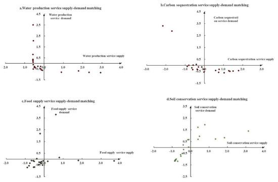
Figure 4.
Supply-demand quadrant chart of (a) water production service, (b) carbon sequestration service, (c) food supply service, and (d) soil conservation service in the ZKL urban agglomeration.
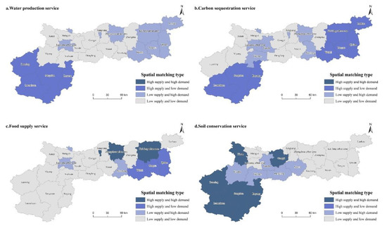
Figure 5.
Supply-demand matching types of (a) water production service, (b) carbon sequestration service, (c) food supply service, and (d) soil conservation service in the ZKL urban agglomeration.
Regarding the water production service, no district or county exhibits high supply–high demand, and low supply–low demand is dominant, as demonstrated by Dengfeng, Xinzheng, Xinmi, Gongyi, Zhongmou, and Xingyang within the scope of Zhengzhou City in the middle section, and Yichuan, Yiyang, Yanshi, Mengjin, and Xin’an within the scope of Luoyang City in the west, i.e., eleven cities or counties. In this area, population density is relatively low. Moreover, rainfall is mostly concentrated during summer and the precipitation is less, leading to low supply of and demand for the water production service. This matching type is followed by low supply–high demand, including the urban area of Zhengzhou, the entirety of Kaifeng City, as well as the urban area of Luoyang, i.e., seven districts or counties. Among them, population aggregation in the urban areas of Zhengzhou and Luoyang has increased due to rapid economic development. Kaifeng is located on the south bank of the lower Yellow River, with fine sand and poor water abundance. Therefore, water yield is low and demand is high in these areas. The regions with high supply–low demand include Luanchuan, Songxian, Ruyang, and Luoning, i.e., four counties in the southwest of Luoyang City. This region has many rivers in mountainous areas and a low population density, resulting in high water yield and low water demand. Water energy resources in Luanchuan are rich, the ecological environment is good, and the conflict between humans and nature is not prominent. This county has the highest water supply, and a mismatch between water production and demand occurs.
With regards to the carbon sequestration service, no district or county exhibits high supply–high demand. Meanwhile, low supply–low demand regions include Dengfeng, Xinmi, Gongyi, Zhongmou, and Xingyang within the scope of Zhengzhou City, and Luoning, Yiyang, Mengjin, and Xin’an within the scope of Luoyang City, i.e., nine cities or counties. In these areas, population density is relatively low and vegetation coverage is low, leading to a low supply of and demand for carbon sequestration service. The high supply–low demand regions include the entirety of Kaifeng City, as well as Luanchun, Songxian, and Ruyang within the scope of Luoyang City, i.e., eight cities or counties. In these areas, vegetation coverage is relatively high, and damage to the habitat caused by human activities is relatively low, resulting in a high supply of and low demand for carbon sequestration. The low supply–high demand regions include the urban area of Zhengzhou and Xinzheng within the scope of Zhengzhou City, and the urban area of Luoyang, Yichuan, and Yanshi within the scope of Luoyang City, i.e., five districts or counties. Energy consumption is high in the urban areas of Zhengzhou and Xinzheng due to their high economic development. Compared with the other cities and counties, the urban areas of Luoyang, Yichuan, and Yanshi have a larger population, with lower vegetation coverage than that in the southwest. Therefore, the carbon sequestration supply is low, and demand is high, in these areas.
Regarding the food supply service, the low supply–low demand type is dominant. These regions comprise 15 cities and counties, including all the district and counties within Zhengzhou City, except for the urban area of Zhengzhou and Xinzheng, and Lankao within Kaifeng City, and all the districts and counties within Luoyang City, except for the urban area of Luoyang. In these areas, population density is relatively low, resulting in low demand for the food supply service. The high supply–low demand regions include Tongxu, Weishi, and Qixian within the scope of Kaifeng City. These areas are rich in agricultural resources and have a strong agricultural foundation. The three counties produce the highest grain output in Kaifeng City. Moreover, population density is low. Therefore, food supply is high and demand is low in these three counties. Tongxu (3.69, −0.15) has rich resources and exhibits high potential in the development of labor-intensive industries. It is the county with the highest supply in the regions. The low supply–high demand regions include Xinzheng within the scope of Zhengzhou City, and the urban area of Luoyang. The quality of cultivated land in these areas is worse than that in other areas. Population is concentrated, resulting in low food supply and high demand.
With regards to the soil conservation service, no district or county exhibits high supply–low demand. Low supply–low demand regions are dominant, and they include the urban area of Zhengzhou, Xinzheng, Zhongmou, and Xingyang within the scope of Zhengzhou City, the entirety of Kaifeng City, as well as the urban area of Luoyang, and Mengjin within the scope of Luoyang City, i.e., 11 districts or counties. In these areas, vegetation coverage is relatively low, leading to low soil conservation and low soil erosion. The high supply–high demand regions include Gongyi within the scope of Zhengzhou City, and Luanchuan, Songxian, Ruyang, Luoning, and Xin’an within the scope of Luoyang City, i.e., six cities and counties. Luanchuan (3.14, 1.39), with a forest coverage rate of 82.4%, ranks first place in Henan Province. It is the county with the highest soil conservation supply in these regions. The low supply–high demand regions include Dengfeng and Xinmi within the scope of Zhengzhou City, and Yichuan, Yiyang, and Yanshi within the scope of Luoyan City, i.e., five cities and counties. Vegetation coverage is low due to the rich mine resources in Dengfeng and Xinmi, and the water and soil protection measures are imperfect. Yichuan, Yiyang, and Yanshi rank as the top three in Luoyang City in terms of population. Damage from human activities to habitats is relatively high. Therefore, soil conservation is low and soil erosion is high in these areas.
4. Discussion
4.1. Supply and Demand (Mis)matches of Ecosystem Services and Their Influencing Factors
ESs are closely related to human well-being. ES mismatches may result in unsatisfied demand. The unsatisfied demand for different ES categories (e.g., food production and soil conservation) can directly impact human well-being. The identification of ES mismatches plays a vital important role in ES decision-making and policy-making [20]. The integrated assessment of ES supply and demand has received widespread attention in recent years [54,55,56,57,58,59,60,61,62,63,64,65,66]. Burkhard et al. [7] proposed a matrix model for quantifying ES supply and demand based on land-use types, which has been applied in many regions [54,55,56,57,58,59]. However, evaluation of ES supply and demand levels using a matrix method provides only relative values, which do not indicate the actual status of supply and demand matching. Furthermore, some studies [60,61] have quantified the supply according to ES value and expressed the demand by the degree of land use and development, population density, and per capita GDP. These quantitative ES supply and demand results do not produce comparable units, so identifying mismatches is difficult. To enable comparison with ES supply, accurate assessment of ecosystem service (ES) demand is a key challenge in this research area. Land-use data, socioeconomic data, or night light data have been applied to quantify ES demand [7,62,63,64,65] but this method is too simplistic and lacks consideration of human needs, complicating the use of such research results in actual management. The demand for provisioning services could be easily captured by examining consumption. For example, the supply-demand ratios of food, energy, and water from 1999 to 2007 in the Leipzig–Halle region of Germany have been quantified to reveal the relationships between land-use change and ESs [66]. However, the regulation of service demands is challenging to evaluate explicitly in the spatial dimension. Our study mapped the supply, demand and matching status of four ESs (i.e., water production, carbon sequestration, food supply, and soil conservation) using biophysical models and the ArcGIS spatial analysis module in the ZKL urban agglomeration. Compared with previous studies on the assessment of ES supply and demand [7,54,55,56,57,58,59,60,61,62,63,64,65,66], our study can be considered an improvement in the following ways. First, it assessed the actual values of ES supply and demand, and the evaluation results in comparable units, which can be used to calculate the supply-demand ratios. Second, it assessed four ESs, including provisioning and regulating services, and integrated sufficient information regarding the supply and demand sides, which could advance the formation of efficient policy.
Our site comprised an urban agglomeration area, and the supply and demand of the ESs studied exhibit evident regional characteristics compared with the economically developed areas with better natural conditions found in southern China [67,68,69]. These characteristics include the following: the supply and demand of ESs in the ZKL area are lower than those in the relatively developed areas in southern China because of the differences between levels of social and economic development and natural resource endowment [68,69]. The supply-demand matching level of some ESs in the ZKL area is lower than that of southern China [68,69]. Water production services are in a deficit state and the supply experiences difficulty in meeting the demand [69]. The different study areas have varying natural, social, and economic characteristics and they have their own significant regional characteristics that govern the spatial differences between the supply and demand of ESs.
Within the international research on ESs, most studies have focused on the supply of ESs alone, and only a few studies have been conducted on the factors that influence the supply-demand relationship of ESs [20]. Thus, quantifying the supply and demand of multiple ESs and analyzing the major influencing factors of supply-demand matching are of considerable practical significance for enriching related research on ESs and facilitating harmonious development between humans and nature. The (mis)matches between the supply and demand of ESs are affected by many factors, such as ecosystem structure and function, ecological processes, population, and economic development. The supply of ESs depends on the conditions of the local natural environment, whereas demand is associated with population growth and socioeconomic development. Climate change and weak ecosystem functions have been identified as natural factors that influence (mis)matches between ES supply and demand [70,71,72]. Land-use change, economic development, and population growth have been identified as human factors that influence (mis)matches between ES supply and demand in time series [73,74]. Our research identified the major factors that influence (mis)matches between ES supply and demand in a spatial dimension. On the basis of the correlation calculation, this study identified six factors that affect the supply-demand ratio of ESs. Based on our findings, the factors that most affect the supply-demand ratio of the food supply service include three natural factors (i.e., elevation, precipitation, and temperature) and three human factors (i.e., population density, GDP, and urbanization level). Natural factors, including temperature, precipitation, and elevation, are the major factors that affect the supply-demand ratio of the water production service. The factors that affect the supply-demand ratio of the carbon sequestration service are mostly human factors, including population density, GDP, and urbanization level. The soil conservation service is mainly affected by the urbanization level, which is belong to the category of human factors. Meanwhile, some scholars have also explored the factors that affect the supply-demand ratio of ESs in some areas. For example, Yang et al. [38] studied the effect of the proportion of construction land and green land on the supply-demand ratio of ESs in Hubei Province. They found a significantly positive correlation between the proportion of green land and the supply-demand ratio of ESs, and a significantly negative correlation between the proportion of construction land and the supply-demand ratio of ESs. The supply-demand ratio of ESs results from the joint influences of the natural environment and social economy. However, the leading factors vary for different ESs. Natural environmental factors are uncontrollable, and thus, it is necessary to focus on human factors in order to improve the supply-demand ratio of ESs in the ZKL urban agglomeration.
4.2. Policy Implications
On the basis of the supply-demand ratio and spatial matching of ESs, the supply-demand state of ESs in the study area can be identified. The states identified can be of three types, namely, supply-demand balance, surplus, and deficit. Simultaneously, four types of areas, namely, low supply–high demand, high supply–high demand, low supply–low demand, and high supply–low demand, are also identified. This study provides a reference for formulating corresponding development guidance strategies and planning recommendations.
Carbon sequestration services in most districts and counties in the ZKL urban agglomeration are in the high surplus state, but the supply-demand ratio in the central urban areas is significantly lower than in the surrounding areas. The supply-demand ratio of the carbon sequestration service is subject to strong impacts from the urbanization level and population density. Therefore, while continuously promoting the construction of green land, afforestation, and other ecological construction, the government should consider promoting green and low-carbon development policies when driving economic growth, evacuating dense populations as appropriate and reducing the proportion of construction land. Simultaneously, effort should be exerted from the demand side to rationally transform modes of development, optimize the industrial structure, and reduce carbon emissions.
The food supply services of the vast majority of districts and counties are in the low surplus state, and thus, food supply faces a particular risk. We should strictly implement a cultivated land protection policy for food supply services to ensure national food security. A strict permanent basic farmland control line and permanent basic farmland protection area should be delimited in the ZKL urban agglomeration. Cultivated land that has been included in the reserve areas should be strictly protected. The local government should continue to promote the construction of high-standard farmland and improve the yield of cultivated land.
The soil conservation services of the vast majority of districts and counties are in the high surplus state. To maintain the current good supply-demand ratio, we should continue implementing some ecological protection policies, such as returning grain plots to forests and closing hillsides to facilitate afforestation. Human activities should be continuously reduced in ecologically fragile and sensitive areas, such as the hilly loess area of Luoyang City and some upstream water source protected areas.
Regarding the balance between supply and demand of ESs, the most serious deficit in the ZKL region is observed in the water production service. The water production service is in a deficit state across a large area of ZKL. The water production service is the most important factor that affects the stability of ESs in the ZKL area. Given the supply-demand matching result for the water production service, the study area is divided into areas of ecological conservation (high supply–low demand), ecological restoration (low supply–high demand), and ecological improvement (low supply–low demand), and the corresponding management countermeasures and measures are proposed (Table 5). In the ecological conservation area (i.e., Luanchuan, Songxian, Ruyang, and Luoning), the government should develop a comprehensive management system with small watersheds as units, and perform ecological conservation through transformation of slopes to ladders, economic fruit forests, soil and water conservation forests, and other measures. The government should actively implement the return of farmland to forests and the closure of mountains to facilitate afforestation. They should also focus on improving the quality of forests, coordinate the restoration of degraded forests, restore ecological forests in mountainous areas, and develop water conservation projects. In the ecological restoration area (i.e., the urban area of Zhengzhou, Luo-yang and Kaifeng, Lankao, Qxian, Tongxu, and Weishi), ecological protection should be taken as the premise of development in future development planning. The government should strictly control urban development boundaries and use the land intensively and economically. Given the positive effects of elevation, precipitation, and temperature on the water production service, we should consider the urban development direction in urban agglomeration planning to prevent water supply shortages from becoming more serious. To alleviate the shortage of water resources, we should strengthen the construction of water conservancy infrastructure, promote a transition in water usage from an extensive to an economical and intensive mode, and enact other relevant water-saving measures, realizing an intensive, safe utilization and rational distribution of water resources. The urban green infrastructure and the area of urban green space should be increased. The core policy of the area should be to control the urbanization process and conduct ecological engineering construction to improve the level of ESs. In the ecological improvement area (i.e., Yiyang, Xin’an, Mengjin, Yichuan, Dengfeng, Yanshi, Gongyi, Xinmi, Zhongmou, Xin-zhang, and Xingyang), the local government should initially focus on adjusting and optimizing the land-use structure and clarifying the agricultural and ecological spaces. We should implement strict ecological protection policies and strictly abide by the ecological bottom line. To improve the utilization efficiency of cultivated-land resources, the existing permanent basic farmland should be strictly protected, and high-standard farmland construction should be conducted. Simultaneously, the local government should promote ecological governance engineering of key waters in the Yellow River, Yihe, and Luohe to improve the utilization efficiency of agricultural water resources. To this end, water-saving technologies should also be developed to further improve agricultural water efficiency.
Table 5.
Ecological subregions and planning recommendations.
4.3. Limitations and Contributions of the Research
Our study applied biophysical models, the ArcGIS spatial analysis module, and four-quadrant analysis in order to identify (mis)matches between ecosystem service supply and demand, and to inform ecological management zoning strategies. However, our study still has some limitations. Firstly, in the biophysical methods, three models (i.e., the InVEST model, CASA model, and RUSLE model) were employed to estimate the supply of water production, carbon sequestration, and soil conservation. Although these ecological models are mature, the ZKL cities represent a special and new area of application, and the estimation results should be validated. However, experimental monitoring data on water production, carbon sequestration, and soil conservation were not available for the ZKL area, meaning this verification process could not be conducted. Secondly, the spatial demand for three ESs (i.e., water production, carbon sequestration, and food supply) were determined based on population patterns and per capita consumption or emissions in our research. The spatial distribution characteristic of ES demand involves many aspects, including social and economic development, personal features (e.g., income, knowledge type, ages and gender), and power relationships [20,75,76,77]. A single population cannot fully capture the spatial heterogeneity of ES demand in the ZKL area, which likely affects the accuracy of the ES demand results. The quantification of ecosystem service demand is a research direction that needs to be improved in the future. There is a need to establish a systematic evaluation system that can consider regional differences in demands for ecosystem services. The establishment of ecosystem service demand indicators should also consider local regional characteristics and differences. In the future, for different ecosystem services, different factors (e.g., population, environmental exposure, and economic development) should be considered to accurately evaluate ecosystem service demand. Moreover, a combination of subjective and objective methods is also important when evaluating ES demand; for instance, a questionnaire survey regarding the demands of stakeholders would complement any objective indicators (e.g., consumption, preference and risk indicators) [78,79,80]. In future research, we will strive to optimize the evaluation of ecosystem service supply and demand.
Despite these limitations, our research methods and results are still conducive to supporting urban ecosystem management. Our results demonstrate that the supply-demand index can satisfactorily depict the matching status of ES supply and demand. It addresses the previous deficiency of research on the quantitative relationship between the supply and demand of ESs and spatial matching in the ZKL urban agglomeration. Our proposed county-based ecological management zoning for ZKL can provide a useful framework to support decision-makers and inform the construction of ecological engineering in these areas. The ZKL area is not only the core economic area in the hinterland of the Central Plains, but is also an important area for ecological protection. It has a high population density, diverse terrain, and a moderately developed economy, as well as complex natural and socioeconomic characteristics. As a typical urban agglomeration in central China in the context of rapid urbanization, ZKL has some reference value for other urban agglomerations in central China. Our study enriches ES research in central China.
5. Conclusions
On the basis of land coverage, meteorological observation, and statistical yearbook data from 2018, this study performed quantitative and visual analysis of four ESs in the ZKL urban agglomeration. We calculated the supply and demand of various ESs using the InVEST, CASA, and RUSLE models, and the ArcGIS spatial analysis module in order to evaluate the supply-demand relationships and examine supply-demand matching of ESs by SDI. Then, we identified the influencing factors and the supply-demand matching types of different ESs in various regions using a four-quadrant analysis. The conclusions drawn are as follows. The supply-demand ratios of different ESs in the cell scale exhibit different spatial characteristics because of differences in the major influencing factors, including the natural environment (e.g., precipitation and temperature) and social development (e.g., urbanization level). The supply-demand ratio of water production is mostly affected by natural factors. It is positively correlated with elevation and precipitation, but negatively correlated with temperature. The supply-demand ratio of carbon sequestration is largely affected by human factors. It is negatively correlated with population density and urbanization level. The major influencing factor of the supply-demand ratios of food supply and soil conservation is urbanization level. Regarding the supply-demand imbalance statuses of the four ESs, water production is deficient across the entire research area, while the carbon sequestration, food supply, and soil conversation of the entire research area are in surplus. The supply and demand matching of ESs in each district and county of ZKL can be divided into four types, according to the spatial differentiation characteristics of supply and demand, as follows: high supply–high demand, low supply–high demand, low supply–low demand, and high supply–low demand. The water production service is dominated by low supply–low demand. The carbon sequestration service is dominated by low supply–low demand and high supply–low demand. The food supply and soil conservation services are dominated by low supply–low demand. All districts and counties in the ZKL urban agglomeration were subsequently divided into areas of ecological conservation, ecological restoration, and ecological improvement, based on the supply and demand matching results of ESs and the severity of the deficit between the supply and demand of the water production service. Considering the different types of ecological areas, development guidance strategies and planning suggestions were proposed.
Ecosystem services are a bridge between natural ecosystems and human society. Their supply and demand reflect the complex relationship between ecosystem services and humans. Our work compensates for the deficiency of research on the quantitative relationship between the supply and demand of ESs and spatial matching in the ZKL urban agglomeration. Development guidance strategies and planning suggestions were proposed for the different types of ecological areas and these policies could also be applied in other similar urban agglomerations. With an increasing population and further enhancement of urban and rural construction, solving the imbalance of ESs in the ZKL area is urgent. In the future, we will establish a systematic evaluation system for the supply and demand of ecosystem services, one which considers regional differences and demands of stakeholders. We will strive to optimize the evaluation of the supply and demand of ecosystem services by combining subjective and objective methods.
Author Contributions
Conceptualization, H.W.; Data curation, D.X.; Formal analysis, D.X.; Funding acquisition, Y.L. and H.W.; Investigation, Z.W.; Project administration, Z.W.; Visualization, M.L.; Writing—original draft, D.X. and Z.W.; Writing—review and editing, H.W. All authors have read and agreed to the published version of the manuscript.
Funding
This research was funded by the National Natural Science Foundation of China (41901259), Second Tibetan Plateau Scientific Expedition and Research Program (2019QZKK0608), Open Fund of Key Laboratory of National Geographical Census and Monitoring, Ministry of Natural Resources (2020NGCM01), and the special fund for top talents in Henan Agricultural University (30500425).
Institutional Review Board Statement
Not applicable.
Informed Consent Statement
Not applicable.
Data Availability Statement
Not applicable.
Conflicts of Interest
The authors declare no conflict of interest.
References
- Wang, J.; Lin, Y.; Zhai, T.; He, T.; Qi, Y.; Jin, Z.; Cai, Y. The role of human activity in decreasing ecologically sound land use in China. Land Degrad. Dev. 2018, 29, 446–460. [Google Scholar] [CrossRef]
- Liu, R.; Dong, X.; Wang, X.C.; Zhang, P.; Liu, M.; Zhang, Y. Study on the relationship among the urbanization process, ecosystem services and human well-being in an arid region in the context of carbon flow: Taking the Manas river basin as an example. Ecol. Indic. 2021, 132, 108248. [Google Scholar] [CrossRef]
- Hu, M.; Wang, Y.; Xia, B.; Jiao, M.; Huang, G. How to balance ecosystem services and economic benefits?—A case study in the Pearl River Delta, China. J. Environ. Manag. 2020, 271, 110917. [Google Scholar] [CrossRef] [PubMed]
- Daily, G.C. Nature’s Services Societal Dependence on Natural Ecosystems; Island Press: Washington, DC, USA, 1997. [Google Scholar]
- Costanza, R.; d’Arge, R.; de Groot, R.; Farber, S.; Grasso, M.; Hannon, B.; Limburg, K.; Naeem, S.; O’Neill, R.V.; Paruelo, J.; et al. The value of the world’s ecosystem services and natural capital. Nature 1997, 387, 256–260. [Google Scholar] [CrossRef]
- Wei, H.; Liu, H.; Xu, Z.; Ren, J.; Lu, N.; Fan, W.; Zhang, P.; Dong, X. Linking ecosystem services supply, social demand and human well-being in a typical mountain-oasis-desert area, Xinjiang, China. Ecosyst. Serv. 2018, 31, 44–57. [Google Scholar] [CrossRef]
- Burkhard, B.; Kroll, F.; Nedkov, S.; Müller, F. Mapping ecosystem service supply, demand and budgets. Ecol. Indic. 2012, 21, 17–29. [Google Scholar] [CrossRef]
- Herreros-Cantis, P.; McPhearson, T. Mapping supply of and demand for ecosystem services to assess environmental justice in New York City. Ecol. Appl. 2021, 31, e02390. [Google Scholar] [CrossRef]
- Rees, W.E. Ecological footprints and appropriated carrying capacity: What urban economics leaves out. Environ. Urban. 1992, 4, 121–130. [Google Scholar] [CrossRef]
- Seidl, I.; Tisdell, C.A. Carrying capacity reconsidered: From Malthus’ population theory to cultural carrying capacity. Ecol. Econ. 1999, 31, 395–408. [Google Scholar] [CrossRef] [Green Version]
- Turner, R.K.; Paavola, J.; Cooper, P.; Farber, S.; Jessamy, V.; Georgiuo, S. Valuing nature: Lessons learned and future research directions. Ecol. Econ. 2003, 46, 493–510. [Google Scholar] [CrossRef] [Green Version]
- Troy, A.; Wilson, M.A. Mapping ecosystem services: Practical challenges and opportunities in linking GIS and value transfer. Ecol. Econ. 2007, 60, 435–449. [Google Scholar] [CrossRef]
- Schulp, C.; Lautenbach, S.; Verburg, P.H. Quantifying and mapping ecosystem services: Demand and supply of pollination in the European Union. Ecol. Indic. 2014, 36, 131–141. [Google Scholar] [CrossRef]
- Sauter, I.; Felix, K.; Bolliger, J.; Winter, B.; Pazúr, R. Changes in demand and supply of ecosystem services under scenarios of future land use in Vorarlberg, Austria. J. Mt. Sci. 2019, 16, 2793–2809. [Google Scholar] [CrossRef]
- Tao, Y.; Wang, H.; Ou, W.; Guo, J. A land-cover-based approach to assessing ecosystem services supply and demand dynamics in the rapidly urbanizing Yangtze River Delta region. Land Use Policy 2018, 72, 250–258. [Google Scholar] [CrossRef]
- Zhang, L.; Fu, B. The progress in ecosystem services mapping: A review. Acta Ecol. Sin. 2014, 34, 316–325. (In Chinese) [Google Scholar]
- Xiao, Y.; Xie, G.; Lu, C.; Xu, J. Involvement of ecosystem service flows in human wellbeing based on the relationship between supply and demand. Acta Ecol. Sin. 2016, 36, 3096–3102. (In Chinese) [Google Scholar]
- Bastian, O.; Syrbe, R.U.; Rosenberg, M.; Rahe, D.; Grunewald, K. The five pillar EPPS framework for quantifying, mapping and managing ecosystem services. Ecosyst. Serv. 2013, 4, 15–24. [Google Scholar] [CrossRef]
- Villamagna, A.M.; Angermeier, P.L.; Bennett, E.M. Capacity, pressure, demand, and flow: A conceptual framework for analyzing ecosystem service provision and delivery. Ecol. Complex 2013, 15, 114–121. [Google Scholar] [CrossRef]
- Wei, H.; Fan, W.; Wang, X.; Lu, N.; Dong, X.; Zhao, Y.; Ya, X.; Zhao, Y. Integrating supply and social demand in ecosystem services assessment: A review. Ecosyst. Serv. 2017, 25, 15–27. [Google Scholar] [CrossRef]
- Compton, J.E.; Harrison, J.A.; Dennis, R.L.; Greaver, T.L.; Hill, B.H.; Jordan, S.J.; Walker, H.; Campbell, H.V. Ecosystem services altered by human changes in the nitrogen cycle: A new perspective for US decision making. Ecol. Lett. 2011, 14, 804–815. [Google Scholar] [CrossRef]
- Dong, X.; Ren, J.; Zhang, P.; Jin, Y.; Liu, R.; Wang, X.-C.; Lee, C.T.; Klemeš, J.J. Entwining ecosystem services, Land Use Change and human well-being by nitrogen flows. J. Clean. Prod. 2021, 308, 127442. [Google Scholar] [CrossRef]
- Ji, Z.; Xu, Y.; Wei, H. Identifying Dynamic Changes in Ecosystem Services Supply and Demand for Urban Sustainability: Insights from a Rapidly Urbanizing City in Central China. Sustainability 2020, 12, 3428. [Google Scholar] [CrossRef] [Green Version]
- Palacios-Agundez, I.; Onaindia, M.; Barraqueta, P.; Madariaga, I. Provisioning ecosystem services supply and demand: The role of landscape management to reinforce supply and promote synergies with other ecosystem services. Land Use Policy 2015, 47, 145–155. [Google Scholar] [CrossRef]
- De Vreese, R.; Leys, M.; Fontaine, C.M.; Dendoncker, N. Social mapping of perceived ecosystem services supply—The role of social landscape metrics and social hotspots for integrated ecosystem services assessment, landscape planning and management. Ecol. Indic. 2016, 66, 517–533. [Google Scholar] [CrossRef]
- Morri, E.; Pruscini, F.; Scolozzi, R.; Santolini, R. A forest ecosystem services evaluation at the river basin scale: Supply and demand between coastal areas and upstream lands (Italy). Ecol. Indic. 2014, 37, 210–219. [Google Scholar] [CrossRef]
- Castro, A.J.; Vaughn, C.C.; Julian, J.P.; García-Llorente, M. Social demand for ecosystem services and implications for watershed management. JAWRA 2016, 52, 209–221. [Google Scholar] [CrossRef]
- Breeze, T.D.; Vaissiere, B.E.; Bommarco, R.; Petanidou, T.; Seraphides, N.; Kozak, L.; Scheper, J.; Biesmeijer, J.C.; Kleijn, D.; Gyldenkaerne, S.; et al. Agricultural policies exacerbate honeybee pollination service supply-demand mismatches across Europe. PLoS ONE 2014, 9, e82996. [Google Scholar] [CrossRef] [Green Version]
- Bagstad, K.J.; Johnson, G.W.; Voigt, B.; Villa, F. Spatial dynamics of ecosystem service flows: A comprehensive approach to quantifying actual services. Ecosyst. Serv. 2013, 4, 117–125. [Google Scholar] [CrossRef]
- Schulp, C.J.E.; Thober, J.; Wolff, S.; Bonn, A. Interregional flows of ecosystem services: Concepts, typology and four cases. Ecosyst. Serv. 2018, 31, 231–241. [Google Scholar]
- Zhang, W.; Wu, X.; Yu, Y. The changes of ecosystem services supply-demand and responses to rocky desertifification in Xiaojiang basin during 2005–2015. J. Soil Water Conserv. 2019, 164, 141–152. (In Chinese) [Google Scholar]
- Yang, L.; Dong, L.; Zhang, L.; He, B.; Zhang, Y. Quantitative assessment of carbon sequestration service supply and demand and service flows: A case study of the Yellow River Diversion Project South Line. Resour. Sci. 2019, 41, 557–571. (In Chinese) [Google Scholar]
- Liu, C.; Wang, W.; Liu, L.; Li, P. Supply-demand matching of county ecosystem services in Northwest China: A case study of Gulang county. J. Nat. Resour. 2020, 35, 2177–2190. (In Chinese) [Google Scholar] [CrossRef]
- Xu, C.; Gong, J.; Yan, L.; Gao, B.; Li, Y. Spatiotemporal changes of supply and demand risk of soil conservation services in Bailongjiang watershed, Gansu Province. Chin. J. Ecol. 2021, 40, 1397–1408. (In Chinese) [Google Scholar]
- Liu, L.; Liu, C.; Wang, C.; Li, P. Supply and demand matching of ecosystem services in loess hilly region: A case study of Lanzhou. Acta Geogr. Sin. 2019, 09, 217–233. (In Chinese) [Google Scholar]
- Cui, F.; Tang, H.; Zhang, Q.; Wang, B.; Dai, L. Integrating ecosystem services supply and demand into optimized management at different scales: A case study in Hulunbuir, China. Ecosyst. Serv. 2019, 39, 100984. [Google Scholar] [CrossRef]
- Xiang, H.; Zhang, J.; Mao, D.; Wang, Z.; Qiu, Z.; Yan, H. Identifying spatial similarities and mismatches between supply and demand of ecosystem services for sustainable Northeast China. Ecol. Indic. 2022, 134, 108501. [Google Scholar] [CrossRef]
- Yang, M.; Zhang, Y.; Wang, C. Spatial-temporal Variations in the Supply-demand Balance of Key Ecosystem Services in Hubei Province. Resour. Environ. Yangtze Basin. 2019, 09, 64–75. (In Chinese) [Google Scholar]
- Yongyong, Z.; Jinjin, H.; Guoxia, M.; Xiaoyan, Z.; Aifeng, L.; Wei, W.; Zhonggen, W. Regional differences of water regulation services of terrestrial ecosystem in the Tibetan Plateau: Insights from multiple land covers. J. Clean. Prod. 2021, 283, 125216. [Google Scholar] [CrossRef]
- Budyko, M.I. Climate and Life. Academy of Sciences, Main Observatory of Leningrad; Academic Press: New York, NY, USA, 1974. [Google Scholar]
- Potter, N.J.; Zhang, L.; Milly, P.C.D.; McMahon, T.A.; Jakeman, A.J. Effects of rainfall seasonality and soil moisture capacity on mean annual water balance for Australian catchments. Water Resour. Res. 2005, 41, W06007. [Google Scholar] [CrossRef] [Green Version]
- Tallis, H.; Ricketts, T.; Guerry, A.; Wood, S.; Sharp, R.; Nelson, E.; Ennaanay, D.; Wolny, S.; Olwero, N.; Vigerstol, K.; et al. InVEST 2.5.3 User’s Guide, the Natural Capital Project; Stanford University: Stanford, CA, USA, 2013. [Google Scholar]
- Meng, S.; Huang, Q.; He, C.; Yang, S. Mapping the Changes in Supply and Demand of Carbon Sequestration Service: A Case Study in Beijing. J. Nat. Resour. 2020, 35, 2177–2190. (In Chinese) [Google Scholar]
- Tu, H.; Liu, C. Calculation of CO2 emission of standard coal. Coal Qual. Technol. 2014, 2, 57–60. (In Chinese) [Google Scholar]
- Zhu, W.; Pan, Y.; Zhang, J. Estimation of Net Primary Productivity of Chinese Terrestrial Vegetation Based on Remote Sensing. Chin. J. Plant Ecol. 2007, 03, 413–424. (In Chinese) [Google Scholar]
- Wang, C.; Liu, C.; Wu, Y.; Liu, Y. Spatial pattern, tradeoffs and synergies of ecosystem services in loess hilly region: A case study in Yuzhong County. Chin. J. Ecol. 2019, 38, 521–531. (In Chinese) [Google Scholar]
- Renard, K.G.; Foster, G.R.; Weesies, G.A.; Porter, J.P. RUSLE: Revised universal soil loss equation. J. Soil Water Conserv. 1991, 46, 30–33. [Google Scholar]
- Chen, J.; Wang, H.; Liu, G.; Bai, Y. Evaluation of Ecosystem Services and Its Adaptive Policies in the Hangjiahu Region under Water-Energy-Food Nexus. Resour. Environ. Yangtze Basin. 2019, 28, 52–63. (In Chinese) [Google Scholar]
- Chen, T.; Feng, Z.; Zhao, H.; Wu, K. Identification of ecosystem service bundles and driving factors in Beijing and its surrounding areas. Sci. Total Environ. 2020, 711, 134687. [Google Scholar] [CrossRef]
- Sannigrahi, S.; Zhang, Q.; Pilla, F.; Joshi, P.K.; Basu, B.; Keesstra, S.; Roy, P.S.; Wang, Y.; Sutton, P.C.; Chakraborti, S.; et al. Responses of ecosystem services to natural and anthropogenic forcings: A spatial regression based assessment in the world’s largest mangrove ecosystem. Sci. Total Environ. 2020, 715, 137004. [Google Scholar] [CrossRef]
- Fang, L.; Wang, L.; Chen, W.; Sun, J.; Cao, Q.; Wang, S.; Wang, L. Identifying the impacts of natural and human factors on ecosystem service in the Yangtze and Yellow River Basins. J. Clean. Prod. 2021, 314, 127995. [Google Scholar] [CrossRef]
- Hu, B.; Kang, F.; Han, H.; Cheng, X.; Li, Z. Exploring drivers of ecosystem services variation from a geospatial perspective: Insights from China’s Shanxi Province. Ecol. Indicat. 2021, 131, 108188. [Google Scholar] [CrossRef]
- Mooney, H.; Larigauderie, A.; Cesario, M.; Elmquist, T.; Hoegh-Guldberg, O.; Lavorel, S.; Mace, G.M.; Palmer, M.; Scholes, R.; Yahara, T. Biodiversity, climate change, and ecosystem services. Curr. Opin. Environ. Sustain. 2009, 1, 46–54. [Google Scholar] [CrossRef]
- Bicking, S.; Burkhard, B.; Kruse, M.; Müller, F. Mapping of nutrient regulating ecosystem service supply and demand on different scales in Schleswig-Holstein, Germany. One Ecosyst. 2018, 3, e22509. [Google Scholar] [CrossRef] [Green Version]
- Schirpke, U.; Candiago, S.; Egarter Vigl, L.; Jäger, H.; Labadini, A.; Marsoner, T.; Meisch, C.; Tasser, E.; Tappeiner, U. Integrating supply, flow and demand to enhance the understanding of interactions among multiple ecosystem services. Sci. Total Environ. 2019, 651, 928–941. [Google Scholar] [CrossRef] [PubMed]
- Wu, A.; Zhao, Y.; Shen, H.; Qin, Y.; Liu, X. Spatio-temporal pattern evolution of ecosystem service supply and demand in Beijing-Tianjin-Hebei region. J. Ecol. Rural Environ. 2018, 34, 968–975. (In Chinese) [Google Scholar]
- He, S.; Su, Y.; Shahtahmassebi, A.R.; Huang, L.; Zhou, M.; Gan, M.; Deng, J.; Zhao, G.; Wang, K. Assessing and mapping cultural ecosystem services supply, demand and flow of farmlands in the Hangzhou metropolitan area, China. Sci. Total Environ. 2019, 692, 756–768. [Google Scholar] [CrossRef] [PubMed]
- Jiang, C.; Yang, Z.; Wen, M.; Huang, L.; Liu, H.; Wang, J.; Chen, W.; Zhuang, C. Identifying the spatial disparities and determinants of ecosystem service balance and their implications on land use optimization. Sci. Total Environ. 2021, 793, 148472. [Google Scholar] [CrossRef] [PubMed]
- Yang, M.; Zhao, X.; Wu, P.; Hu, P.; Gao, X. Quantification and spatially explicit driving forces of the incoordination between ecosystem service supply and social demand at a regional scale. Ecol. Indicat. 2022, 137, 108764. [Google Scholar] [CrossRef]
- Xu, Q.; Yang, R.; Zhuang, D.; Lu, Z. Spatial gradient differences of ecosystem services supply and demand in the pearl river delta region. J. Clean. Prod. 2020, 279, 123849. [Google Scholar] [CrossRef]
- Peng, J.; Yang, Y.A.; Xie, P.; Liu, Y.X. Zoning for the construction of green space ecological networks in Guangdong Province based on the supply and demand of ecosystem services. Acta Ecol. Sin. 2017, 37, 4562–4572. (In Chinese) [Google Scholar]
- Li, K.; Hou, Y.; Andersen, P.S.; Xin, R.; Rong, Y.; Skov-Petersen, H. An ecological perspective for understanding regional integration based on ecosystem service budgets, bundles, and flows: A case study of the Jinan metropolitan area in China. J. Environ. Manag. 2022, 305, 114371. [Google Scholar] [CrossRef]
- Wang, M.; Bai, Z.; Dong, X. Land Consolidation Zoning in Shaanxi Province based on the Supply and Demand of Ecosystem Services. Chin. Land Sci. 2018, 32, 73–80. (In Chinese) [Google Scholar] [CrossRef] [Green Version]
- Gu, K.; Yang, Q.; Cheng, F.; Chu, J.; Chen, X. Spatial Differentiation of Anhui Province Based on the Relationship between Supply and Demand of Ecosystem Services. J. Ecol. Rural Environ. 2018, 34, 577–583. (In Chinese) [Google Scholar]
- Huang, Z.; Wang, F.; Cao, W. Dynamic analysis of an ecological security pattern relying on the relationship between ecosystem service supply and demand:a case study on the Xiamen-Zhangzhou-Quanzhou city cluster. Acta Ecol. Sin. 2018, 38, 4327–4340. (In Chinese) [Google Scholar]
- Kroll, F.; Müller, F.; Haase, D.; Fohrer, N. Rural–urban gradient analysis of ecosystem services supply and demand dynamics. Land Use Policy 2012, 29, 521–535. [Google Scholar] [CrossRef]
- Dong, X.; Xie, M.; Zhang, Q.; Wang, M.; Guo, X. Ecosystem services demand assessment regarding disaster vulnerability and supply-demand spatial matching. Acta Ecol. Sin. 2018, 38, 6422–6431. (In Chinese) [Google Scholar]
- Liu, S.; Yang, Y.; Wang, Y. Mapping supply and demand differentiation of hydrological regulation service based on matrix analysis: A case study of Jiaxing City, Zhejiang Province. Acta Ecol. Sin. 2019, 39, 1189–1202. (In Chinese) [Google Scholar]
- Wu, J.; Men, X.; Liang, J.; Zhao, Y. Research on supply and demand equilibrium of ecosystem services in Guangdong Province based on the gini coefficient. Acta Ecol. Sin. 2020, 40, 6812–6820. (In Chinese) [Google Scholar]
- Baró, F.; Haase, D.; Gómez-Baggethun, E.; Frantzeskaki, N. Mismatches between ecosystem services supply and demand in urban areas: A quantitative assessment in five European cities. Ecol. Indic. 2015, 55, 146–158. [Google Scholar] [CrossRef] [Green Version]
- Beichler, S.A. Exploring the link between supply and demand of cultural ecosystem services—Towards an integrated vulnerability assessment. Int. J. Biodiv. Sci. Ecosyst. Serv. Manage. 2015, 11, 250–263. [Google Scholar] [CrossRef]
- Quintas-Soriano, C.; Castro, A.J.; García-Llorente, M.; Cabello, J.; Castro, H. From supply to social demand: A landscape-scale analysis of the water regulation service. Landsc. Ecol. 2014, 29, 1069–1082. [Google Scholar] [CrossRef]
- Vigl, L.E.; Depellegrin, D.; Pereira, P.; de Groot, R.; Tappeiner, U. Mapping the ecosystem service delivery chain: Capacity, flow, and demand pertaining to aesthetic experiences in mountain landscapes. Sci. Total Environ. 2017, 574, 422–436. [Google Scholar] [CrossRef]
- Stürck, J.; Schulp, C.J.E.; Verburg, P.H. Spatio-temporal dynamics of regulating ecosystem services in Europe—The role of past and future land use change. Appl. Geogr. 2015, 63, 121–135. [Google Scholar] [CrossRef]
- Felipe-Lucia, M.R.; Martin-Lopez, B.; Lavorel, S.; Berraquero-Diaz, L.; Escalera-Reyes, J.; Comin, F.A. Ecosystem services flows: Why stakeholders’ power relationships matter. PLoS ONE 2015, 10, e0132232. [Google Scholar] [CrossRef] [PubMed] [Green Version]
- Lin, Y.; Chen, X.; Huang, L.; Zhu, C.; Shahtahmassebi, A.; Zhang, J.; Shen, S.; Peng, R.; Deng, J.; Wang, K.; et al. Fine-scale mapping of urban ecosystem service demand in a metropolitan context: A population-income-environmental perspective. Sci. Total Environ. 2021, 781, 146784. [Google Scholar] [CrossRef]
- Meng, Q.; Zhang, L.; Wei, H.; Cai, E.; Xue, D.; Liu, M. Linking Ecosystem Service Supply–Demand Risks and Regional Spatial Management in the Yihe River Basin, Central China. Land 2021, 10, 843. [Google Scholar] [CrossRef]
- Sun, R.; Li, F.; Chen, L. A demand index for recreational ecosystem services associated with urban parks in Beijing, China. J. Environ. Manag. 2019, 251, 109612. [Google Scholar] [CrossRef]
- Zhao, Y.; Wang, N.; Luo, Y.; He, H.; Wu, L.; Wang, H.; Wang, Q.; Wu, J. Quantification of ecosystem services supply-demand and the impact of demographic change on cultural services in Shenzhen, China. J. Environ. Manag. 2022, 304, 114280. [Google Scholar] [CrossRef]
- Zoderer, B.M.; Tasser, E.; Carver, S.; Tappeiner, U. Stakeholder perspectives on ecosystem service supply and ecosystem service demand bundles. Ecosyst. Serv. 2019, 37, 100938. [Google Scholar] [CrossRef]
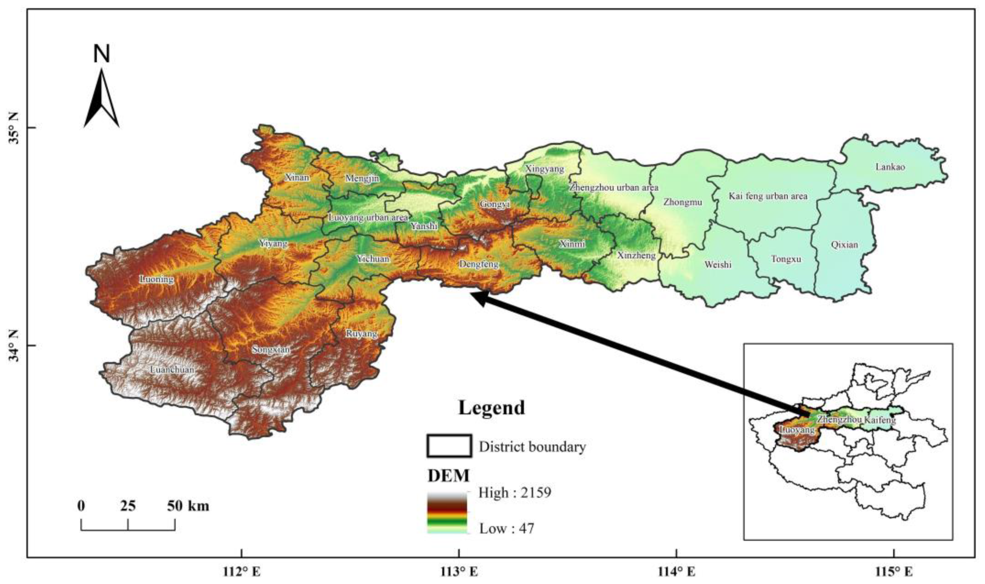
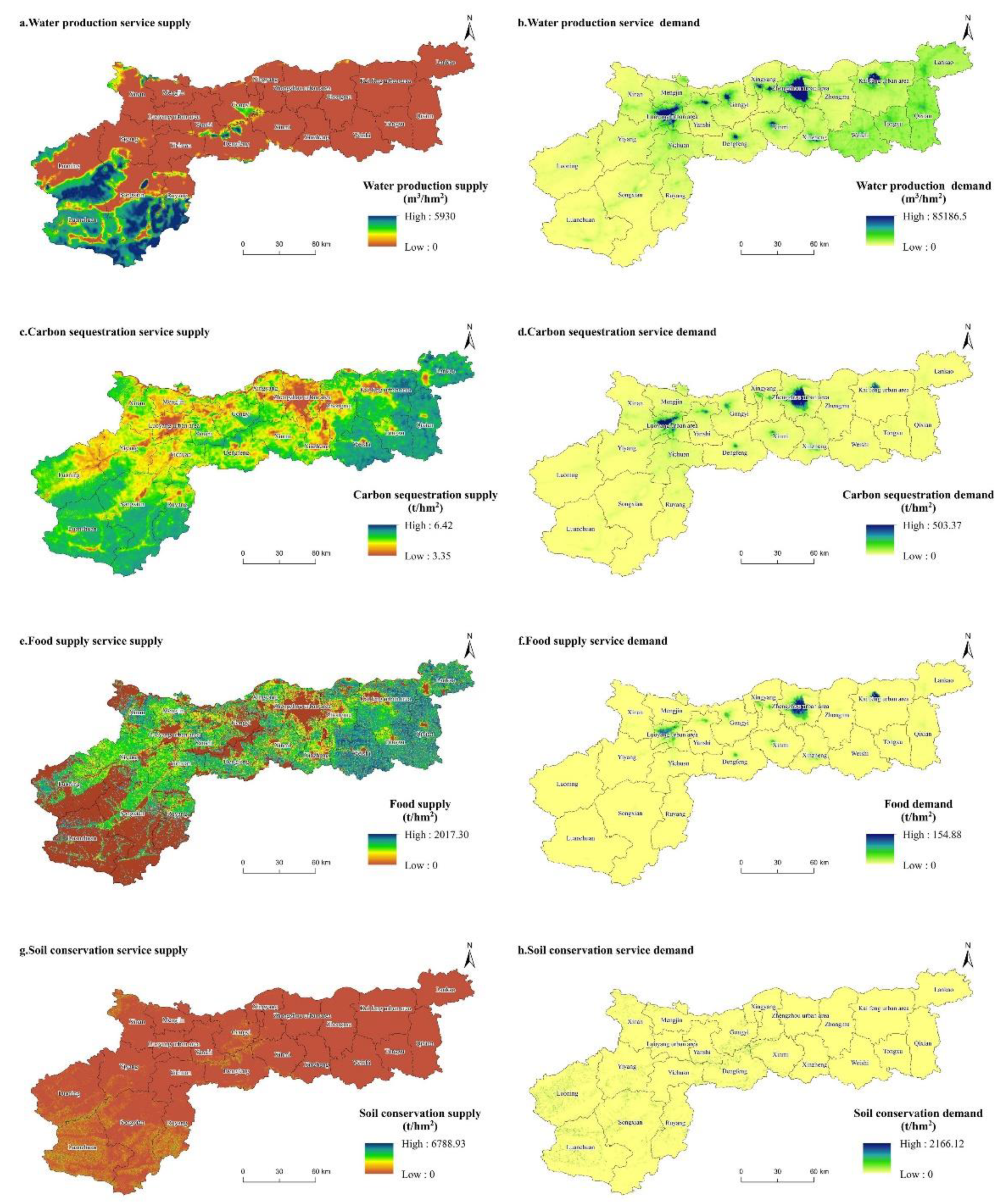
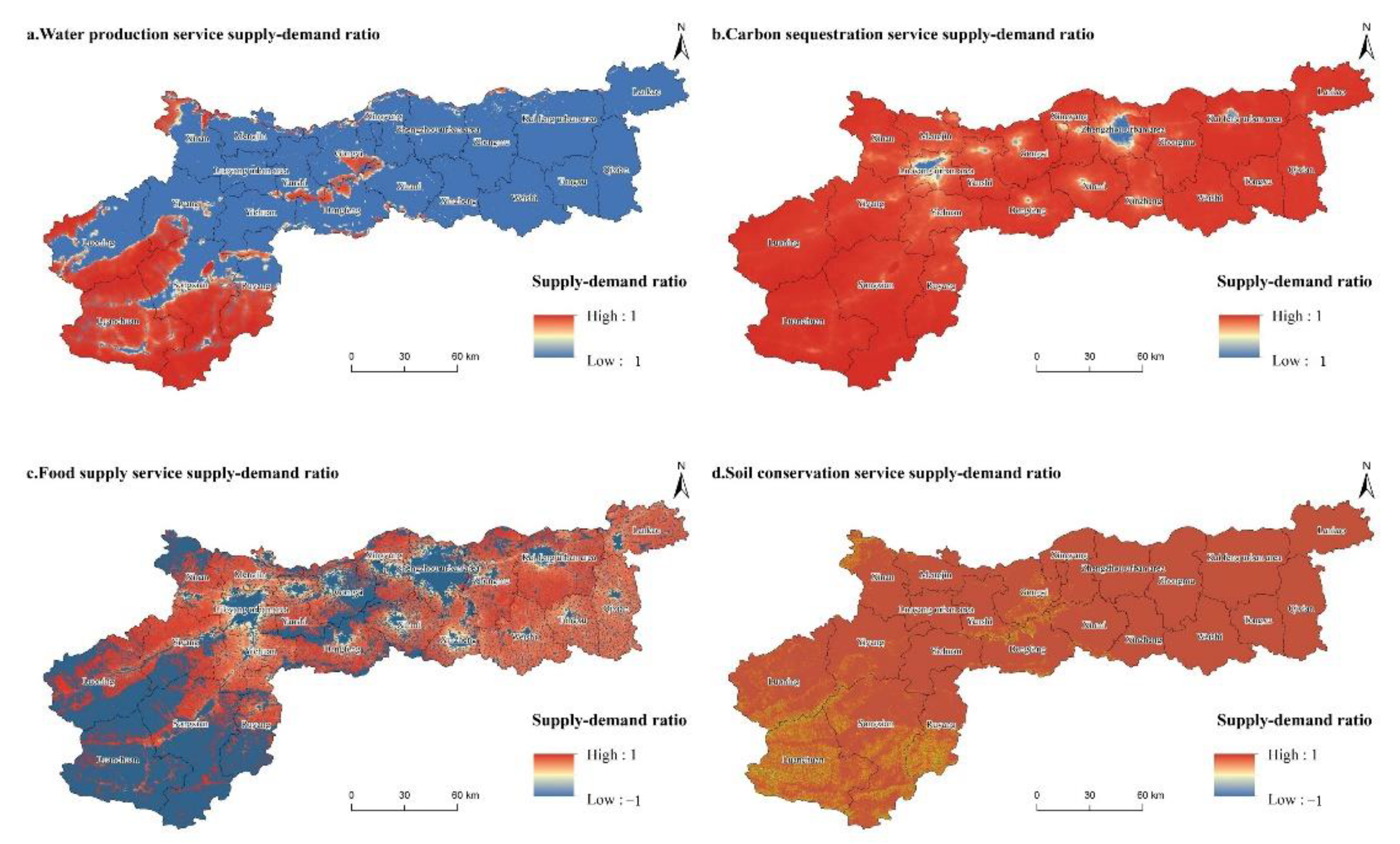
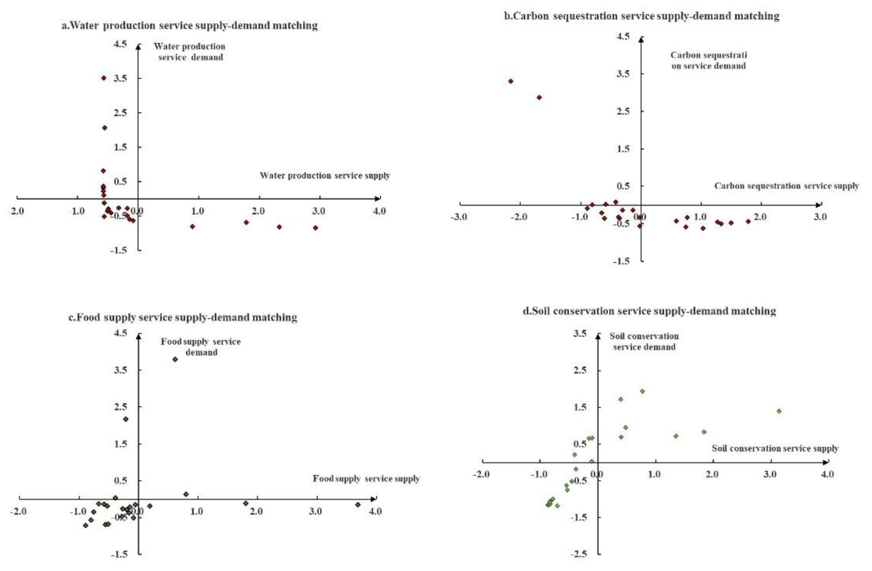

Publisher’s Note: MDPI stays neutral with regard to jurisdictional claims in published maps and institutional affiliations. |
© 2022 by the authors. Licensee MDPI, Basel, Switzerland. This article is an open access article distributed under the terms and conditions of the Creative Commons Attribution (CC BY) license (https://creativecommons.org/licenses/by/4.0/).