A Spatiotemporal Network Model for Global Ionospheric TEC Forecasting

Abstract

In the Global Navigation Satellite System, ionospheric delay is a significant source of error. The magnitude of the ionosphere total electron content (TEC) directly impacts the magnitude of the ionospheric delay. Correcting the ionospheric delay and improving the accuracy of satellite navigation positioning can both benefit from the accurate modeling and forecasting of ionospheric TEC. The majority of current ionospheric TEC forecasting research only considers the temporal or spatial dimensions, ignoring the ionospheric TEC’s spatial and temporal autocorrelation. Therefore, we constructed a spatiotemporal network model with two modules: (i) global spatiotemporal characteristics extraction via forwarding spatiotemporal characteristics transfer and (ii) regional spatiotemporal characteristics correction via reverse spatiotemporal characteristics transfer. This model can realize the complementarity of TEC global spatiotemporal characteristics and regional spatiotemporal characteristics. It also ensures that the global spatiotemporal characteristics of the global ionospheric TEC are transferred to each other in both temporal and spatial domains at the same time. The spatiotemporal network model thus achieves a spatiotemporal prediction of global ionospheric TEC. The Huber loss function is also used to suppress the gross error and noise in the ionospheric TEC data to improve the forecasting accuracy of global ionospheric TEC. We compare the results of the spatiotemporal network model with the Center for Orbit Determination in Europe (CODE), the convolutional Long Short-Term Memory (convLSTM) model and the Predictive Recurrent Neural Network (PredRNN) model for one-day forecasts of global ionospheric TEC under different conditions of time and solar activity, respectively. With internal data validation, the average root mean square error (RMSE) of our proposed algorithm increased by 21.19, 15.75, and 9.67%, respectively, during the maximum solar activity period. During the minimum solar activity period, the RMSE improved by 38.69, 38.02, and 13.54%, respectively. This algorithm can effectively be applied to ionospheric delay error correction and can improve the accuracy of satellite navigation and positioning.

1. Introduction

The ionosphere is an important part of the atmospheric space layer. It contains many free electrons and ions, which are refracted by traversing wireless signals. Therefore, it affects the accuracy of Earth-space-based application systems such as satellite positioning, navigation, time service, and remote sensing systems [1]. In the Global Navigation Satellite System (GNSS), the satellite carrier and pseudo-range signals received by ground stations are affected by the ionosphere with time-delay effects of up to several tens of meters [2]. This seriously affects the accuracy and precision of satellite navigation and positioning. Total electron content (TEC) is the sum of free electrons in a path between the satellite and the receiver [3] and is an important parameter describing the morphology and structure of the ionosphere. The effect of the ionosphere on satellite signals is proportional to TEC. Ionospheric TEC can be used to analyze ionospheric activity and its variation patterns at different spatial and temporal scales. A more accurate ionospheric TEC forecast model, which can be used for ionospheric delay correction, to mitigate the impact of the ionosphere on satellite signals and improve the accuracy of satellite navigation and positioning is required. The accurate modeling and forecasting of TEC are critical for satellite positioning, navigation, measurement and control, and the time-frequency transmission of radio wave propagation over the satellite–ground link.

The ionosphere is a highly dynamic environment that undergoes significant spatial and temporal variability with changes in latitude, longitude, time, and season. Therefore, the magnitude of ionospheric TEC is highly dependent on time, latitude, longitude, season, solar activity, and geomagnetic conditions, and the temporal and spatial dimensions are interdependent. It contains spatiotemporal series data with spatiotemporal-varying characteristics and high autocorrelation. As a result of these factors, the ionosphere is highly variable, making it difficult to establish a global high-precision ionospheric TEC forecast model.

Many scholars have conducted several studies on ionospheric TEC forecasting. The Committee on Space Research and the International Union of Radio Science collaborated on the first studies with Rawer et al., proposing the International Reference Ionosphere (IRI) model based on empirical modeling [4]. In addition to the IRI model, the Bent model [5], the Klobuchar model [6], and the NeQuick model [7] are also widely used in satellite signal delay correction. The Klobuchar broadcast model and the NeQuick broadcast model were used by the Global Positioning System (GPS) and Galileo positioning system, respectively, to estimate ionospheric parameters for single-frequency users [8]. All these models are global empirical models that fit the ionospheric TEC well for a global region but are less accurate for local regions. These models may obliterate features that are unique to certain regions [9], especially in the presence of perturbation conditions in the ionosphere [10]. In such cases, regional or local models are more advantageous in characterizing the ionosphere [11]. For modeling ionospheric TEC in local regions, linear models such as the autoregressive (AR) model and autoregressive moving average (ARMA) model for time series prediction are used [12,13]. However, these models are linear regressions for the time domain, do not capture abrupt changes in ionospheric TEC, and cannot fit ionospheric TEC in the highly nonlinear relationship [14].

In addition, the ionospheric TEC can be obtained by using the linear combination of the observed data of the multi-frequency GNSS with a single constellation and/or multiple constellations [15,16,17]. Based on this computational process, the Ionospheric Associate Analysis Centers (IAACs) of the International GNSS Service (IGS) use TEC data from hundreds of IGS observatories worldwide using different methods and techniques to construct a global ionospheric model [18]. They also produce global ionospheric maps, which have been widely used for ionospheric error removal in single-frequency and dual-frequency precise point positioning [19]. These IAACs also offer prediction products for ionospheric TEC, obtained by extrapolation methods or based on physical model calculations. For example, the prediction products of the Centre for Orbit Determination in Europe (CODE), one of the IAACs, are obtained by the extrapolation of spherical harmonic coefficients [20]. The ionospheric prediction model of the Universitat Politècnica de Catalunya (UPC), on the other hand, is based on linear regression and discrete cosine transform [21]. The global ionospheric maps predicted by CODE also have a higher accuracy than the global ionospheric TEC maps predicted by two IAACs, UPC and the European Space Operations Center of the European Space Agency (ESA) [22].

Artificial intelligence technology has advanced in leaps and bounds since the dawn of the big data era and the introduction of high-performance GPUs. In recent years, many researchers have used machine learning algorithms to study ionospheric TEC forecasting. Feedforward neural networks, which consist of multiple interconnected artificial neurons, are capable of fitting nonlinear relationships in data [23], and several studies have used a feedforward neural network to build ionospheric TEC models [24,25,26]. Feedforward neural networks are capable of approximating nonlinear ARMA relationships, thus improving the performance of ionospheric TEC modeling. Radial basic function (RBF), support vector machines (SVM), and fully connected neural networks have also been applied in ionospheric TEC modeling studies [27,28,29]. Global ionospheric TEC models have also been developed using parameters such as the geomagnetic index and solar activity index using EXtreme Gradient Boosting over Decision Trees techniques [30]. However, the above algorithms lack a circular feedback mechanism between artificial neurons, are unable to better suit temporal correlation and mutability in time-series data, and have unstable convergence.

For this reason, deep learning is gradually being used as an alternative paradigm to machine learning [31]. Compared to machine learning, deep learning is not only capable of mining valid information from data and automatically capturing hidden linear and non-linear features in data, but can also efficiently process large-scale spatiotemporal sequence data [32]. As one of the deep learning algorithms, the recurrent neural network (RNN) establishes a recurrent feedback mechanism between neurons and can fit temporal correlations in time-series data, which can be used for ionospheric TEC modulation. However, RNN suffers from gradient disappearance during the learning process and is unable to fit complex temporal correlations. Long short-term memory (LSTM) was proposed [33] to solve the problem of RNN gradient disappearance while retaining the advantages of RNN in terms of fitting temporal correlations. Many scholars have used correlation factors such as latitude, longitude, time, and geomagnetic index as input parameters for the LSTM model to build ionospheric TEC forecasting models [34,35,36,37].

Although LSTM models can fit ionospheric TEC models well, they mainly fit the temporal dimension of ionospheric TEC. However, spatial factors such as latitude and longitude have an impact on ionospheric TEC. The traditional LSTM models are less likely to learn the spatial characteristics of ionospheric TEC and lack the fitting of the spatial dimension of ionospheric TEC. This reduces the accuracy of ionospheric TEC forecasting models by ignoring the spatial and temporal autocorrelation therein. Furthermore, some researchers have also modeled ionospheric TEC maps as two-dimensional images and fitted the spatial features in them to predict ionospheric TEC maps [38,39]. However, they neglected the effect of time on ionospheric TEC and similarly did not consider the spatiotemporal autocorrelation, which influenced the forecasting accuracy.

In deep learning, RNN or LSTM focus more on modeling time series but lack attention to spatial features, resulting in blurred images. Convolutional neural networks (CNNs) focus more on extracting spatial features but are relatively weak at capturing time. At the same time, neither RNN nor CNN can effectively capture the temporal variability and spatial features of spatiotemporal sequence data. To address this problem, some scholars proposed combining the use of RNN and CNN to capture the spatiotemporal features of spatiotemporal sequence data. One of them introduced convolutional operations into LSTM to construct convolutional LSTM (convLSTM) structures. This scholar also built an encoder–decoder prediction model by stacking convLSTM units [40] to effectively extract the spatiotemporal variation features of the data. Similarly, this algorithm has been applied to the study of global ionospheric TEC forecasting. convLSTM units can be used to learn the time-varying properties and spatial characteristics of global ionospheric TEC and fit non-linear relationships such as the spatiotemporal autocorrelation [41,42]. However, in the process of extracting spatiotemporal information from the convLSTM units, the stacked convLSTM units are independent of each other. The time-varying characteristics of the ionospheric TEC can only be horizontally transferred in the time domain, and the spatial features can only be vertically transferred in the spatial domain. Therefore, the spatiotemporal features cannot be transferred to each other in the time and spatial domains at the same time. Additionally, the historical spatiotemporal information applied to the current moment is incomplete. This reduces the accuracy of the resulting forecast.

To address the aforementioned issues, one researcher created a Spatiotemporal Long Short-Term Memory (ST-LSTM) unit by adding spatiotemporal memory modules to the convLSTM unit. The Predictive Recurrent Neural Network (PredRNN) [43] was built by stacking the ST-LSTM units. This model ensures that the spatiotemporal features are simultaneously passed to each other in the time and space domains to improve forecast accuracy. However, the low-layer ST-LSTM units in the PredRNN model have incomplete spatiotemporal properties and lack the global spatiotemporal features on which the forecast results are more dependent.

Therefore, in light of the spatiotemporal characteristics of ionospheric TEC, we employed the ST-LSTM unit to learn the time-varying and spatial characteristics of the global ionospheric TEC. Two modules were established for global spatiotemporal characteristics extraction via forwarding spatiotemporal characteristics transfer and regional spatiotemporal characteristics correction via reverse spatiotemporal characteristics transfer. In this way, a spatiotemporal network model of the global ionospheric TEC is constructed to compensate for the low-layer ST-LSTM units’ deficiencies in spatiotemporal characteristics. In addition, this achieves complementarity of the global spatiotemporal characteristics and regional spatiotemporal characteristics of the TEC, ensuring that global spatiotemporal properties are simultaneously transferred in the time and space domains. This can improve the model’s ability to fit non-linear relationships, such as TEC’s spatiotemporal autocorrelation, and achieve a spatiotemporal prediction of global ionospheric TEC. Meanwhile, for the non-linear, non-smooth, and highly noisy characteristics of global ionospheric TEC data [44], we used the Huber loss function [45] to constrain the model training process, suppressing the gross error and noise in global ionospheric TEC data and further improving the forecast accuracy of global ionospheric TEC.

To validate the forecast performance of the global ionospheric TEC, our proposed algorithm is used to forecast the future day variability of the global ionospheric TEC. At different times and under different solar activity conditions, we first performed an internal validation using the IGS final TEC test set data. The one-day forecasts were compared with those of the CODE, convLSTM model, and PredRNN model for visual and quantitative evaluation. This was followed by external validation using altimetric satellite vertical total electron content (VTEC) data for a quantitative comparison with the one-day forecast results from CODE and forecast performance when subjected to severe solar storm disturbances. The results of the experiments show that our method can improve the global ionospheric TEC forecast accuracy and can be used to correct ionospheric delay errors in satellite navigation positioning. The remainder of this article is structured as follows: Section 2 introduces the global ionospheric TEC data used in our paper, Section 3 describes the specific principles of our method, Section 4 presents the experimental results and compares and analyses the forecast performance of several algorithms, and Section 5 concludes with the appropriate conclusions.

2. Database

The TEC data provided by the IGS are calculated from the observations from several hundred IGS observatories around the world, which have high accuracy and can be used as reference data for experiments. The distribution of global IGS stations is shown in Figure 1. IGS produces a rapid TEC and final TEC. They are obtained through different IAACs using different global ionospheric model calculations. There is consistency between the results of individual IAAC with comparable accuracy [46]. In contrast, the IGS-combined TEC products have a higher accuracy than those of any individual IAAC [47]. In addition, the rapid TEC has a delay of fewer than 24 h, but its accuracy is 10~15% lower than the final TEC, which has higher accuracy and reliability, but a delay of about 11 days [39]. Therefore, we used the final TEC of the IGS combination of the maximum solar activity period (1 January 2013~31 December 2014) and minimum solar activity period (1 January 2017~31 December 2018) as the experimental dataset to validate the forecast performance of the spatiotemporal network model. The final TEC of the IGS combination was obtained from NASA’s Crustal Dynamics Data Information System (CDDIS) website (https://cddis.nasa.gov/archive/gnss/products/ionex/) (accessed on 20 December 2021). One-day forecasts of CODE for the comparison experiments were also obtained from the CDDIS website.

The IGS provided a standard IONospheric EXchange (IONEX) file that was used to generate a global ionospheric TEC spatiotemporal series. It had a temporal resolution of 2 h, including 0 h and 24 h, for a total of 13 global ionospheric TEC maps per day. The longitude ranged from 180°W to 180°E, with a 5° spatial resolution, and the latitude ranged from 87.5°N to 87.5°S, with a 2.5° spatial resolution. Figure 2 shows a standard global ionospheric TEC map as an example. The global ionospheric TEC map is preprocessed by removing data from duplicate positions in each global ionospheric TEC map and replacing the positions with the null value with 0 to obtain a global ionospheric TEC map of size 72 × 72.

In the experiment, global ionospheric TEC data are processed into a spatiotemporal sequence every four days. The global ionospheric TEC of the previous three days formed the historical observations that were used to predict the global ionospheric TEC of the next day, i.e., each sequence contains a total of 52 global ionospheric TEC maps, thus constituting a global ionospheric TEC spatiotemporal sequence dataset. The training set included global ionospheric TEC data from 1 January 2013 to 19 November 2014 and 1 January 2017 to 19 November 2018, totaling 17,888 global ionospheric TEC maps. The global ionospheric TEC data from 20 November 2014 to 31 December 2014 and 20 November 2018 to 31 December 2018 were used as two test sets. Each test set contained 546 global ionospheric TEC maps to validate the forecasting performance of the spatiotemporal network model for periods of maximum solar activity and minimum solar activity, respectively.

3. Method

The ionospheric TEC value is highly dependent on time, latitude, longitude, season, solar activity, and geomagnetic conditions. There are interdependencies between the temporal and spatial dimensions, as well as spatial and temporal variability, and a high degree of autocorrelation. With a one-dimensional time dimension and a two-dimensional spatial dimension, this is a three-dimensional spatiotemporal tensor. The global ionospheric TEC at each moment is a two-dimensional spatial image of size $M\times N$, containing $P$ different TEC features. For any moment in time, the global ionospheric TEC observations can be expressed using a tensor $X$ as $X\in R^{P\times M\times N}$, where $R$ is the domain of the TEC features. As the global ionospheric TEC observations are recorded over time, a spatiotemporal tensor sequence $X_1,X_2,\dots X_t$ is obtained. Using the global ionospheric TEC observations for the previous $J$ moments, including the current moment, as historical data, the global ionospheric TEC values for the next $K$ moments are predicted and can be expressed as:

$${\widehat{X}}_{t+1},\dots ,{\widehat{X}}_{t+K}=\underset{X_{t+1},\dots ,X_{t+K}}{\arg \max }\rho (X_{t+1},\dots ,X_{t+K}|X_{t-J+1},\dots ,X_t)$$

(1)

The above equation, $\widehat{X}$, represents the global ionospheric TEC prediction, $X$ represents the actual observation, and $\rho$ is the established ionospheric TEC forecast model, which, in this paper, is our spatiotemporal network forecast model. We used $K=13$, $J=39$ and $t=39$, i.e., we used the global ionospheric TEC observations of the previous three days to predict the global ionospheric TEC changes for the following day.

3.1. Spatiotemporal Network Model

As previously stated, traditional LSTM models mainly fit the time dimension of the ionospheric TEC and lack the spatial dimension fitting of the ionospheric TEC. The spatial and temporal autocorrelation is neglected in the TEC. Although the model with stacked convLSTM units can simultaneously learn the time-varying characteristics and spatial features of the ionospheric TEC, the convLSTM units are independent of each other. The time-varying characteristics of the ionospheric TEC can only be horizontally transferred in the time domain and the spatial features can only be vertically transferred in the spatial domain. Therefore, the spatiotemporal features cannot be transferred to each other in the time and spatial domains at the same time, which affects the forecast accuracy.

The PredRNN model for spatiotemporal sequence prediction constructs an ST-LSTM by adding a spatiotemporal memory module to the convLSTM unit. Four ST-LSTM units are stacked to build a network where spatiotemporal features are simultaneously passed to each other in the temporal and spatial domains, which jointly act on the forecast results. Therefore, we first used the ST-LSTM unit to learn the global ionospheric TEC’s time-varying properties, spatial characteristics, and fitting non-linear relationships, such as the spatiotemporal autocorrelation of the global ionospheric TEC.

Figure 3 depicts the internal structure of the ST-LSTM unit, with the expression:

$$\begin{array}{l}{g}_t=\tanh (W_{xg}*X_t+W_{hg}*H_{t-1}^l+b_g)\\ i_t=\sigma (W_{xi}*X_t+W_{hi}*H_{t-1}^l+b_i)\\ f_t=\sigma (W_{xf}*X_t+W_{hf}*H_{t-1}^l+b_f)\\ C_t^l=f_t\odot C_{t-1}^l+i_t\odot g_t\\ g_t^{’}=\tanh (W_{xg}^{’}*X_t+W_{mg}^{’}*M_t^{l-1}+b_g^{’})\\ i_t^{’}=\sigma (W_{xi}^{’}*X_t+W_{mi}^{’}*M_t^{l-1}+b_i^{’})\\ f_t^{’}=\sigma (W_{xf}^{’}*X_t+W_{mf}^{’}*M_t^{l-1}+b_f^{’})\\ M_t^l=f_t^{’}\odot M_t^{l-1}+i_t^{’}\odot g_t^{’}\\ o_t=\sigma (W_{xo}*X_t+W_{ho}*H_{t-1}^l+W_{co}*C_t^l+W_{mo}*M_t^l+b_o)\\ H_t^l=o_t\odot \tanh (W_{1\times 1}*\left[C_t^l,M_t^l\right])\end{array}$$

(2)

In Equation (2), $f,i,g$ denote the forgetting gate, the input gate, and the input modulation gate of the original convLSTM part of the ST-LSTM unit, respectively. The forgetting gate determines the effect of the previous spatiotemporal characteristics on the current epoch and decides whether the previous spatiotemporal characteristics are retained for further input into the current moment. The input modulation gate assists the input gate in determining how many of the spatiotemporal characteristics can be deposited into the current cell state; i.e., the weight of each spatiotemporal characteristic is determined. $f’,i’,g’$ denote the forgetting gate, the input gate, and the input modulation gate of the new temporal memory module in the ST-LSTM unit, respectively, with the same role as $f,i,g$. $o$ represents the output gate, which determines how many hidden states can be output at the current moment, and based on the currently hidden states, the prediction can be calculated. $l$ is the number of layers in the ST-LSTM unit stack, t denotes the current moment, and W and b with different subscripts correspond to the convolution kernel and bias in each convolution operation, respectively. X represents the input data, $\sigma$ and tanh are the different activation functions, $\odot$ is the Hadamard product, and $*$ is the convolution operator. $C_t^l$ and $M_t^l$ are the two memory storage units of the ST-LSTM unit, colloquially known as the structure used for storing the learned spatiotemporal characteristics. $H_t^l$ represents the hidden state of the ST-LSTM unit, which affects the prediction results. $C_t^l$ is the same as the cell state of the original convLSTM and is mainly responsible for the horizontal transference of temporal memory between the preceding and following moments, i.e., ensuring that the time-varying characteristics of the ionospheric TEC are horizontally transferred in the time domain. $M_t^l$ is a new spatiotemporal memory cell state in the ST-LSTM. It is mainly responsible for the transference of spatiotemporal memory, which is vertically transferred into the ST-LSTM units of different layers at the same moment, and into the ST-LSTM units of the underlying layer at the next moment. This means that the spatiotemporal characteristics of the ionospheric TEC are guaranteed to be simultaneously transmitted in the time and space domains, when $l=1$, $M_t^{l-1}=M_{t-1}^L$. The final hidden state of the ST-LSTM unit relies on the fusion of spatiotemporal memory. By concatenating the time-varying and spatiotemporal characteristics of the ionospheric TEC, and then using a 1 × 1 convolutional layer for dimensionality reduction, the final hidden state is obtained, which determines the forecast results of the global ionospheric TEC. The global ionospheric TEC forecast results can be calculated from the following equation:

$${\widehat{X}}_{t+1}=W_{1\times 1}*H_t^{l=4}$$

(3)

The local spatial features of different regions of the ionospheric TEC are gradually extracted by the convolution operation in the ST-LSTM units. The LSTM structure in it gradually learns the time-varying characteristics of the ionospheric TEC. Together, these constitute the regional spatiotemporal signature of the ionospheric TEC. As the ST-LSTM units are continuously stacked, the different regional spatiotemporal features gradually converge into the top-layer ST-LSTM, which constitutes the global spatiotemporal properties of the ionospheric TEC on a global scale. Thus, the top-layer ST-LSTM unit at each moment contains the richest TEC global spatiotemporal properties. Through the newly added spatiotemporal memory module in the ST-LSTM unit, the global spatiotemporal properties of the top layer are transferred to the bottom-layer ST-LSTM unit at the next moment. This enables the transference of the spatiotemporal properties of the ionospheric TEC in different spatial and temporal dimensions.

In the process of learning the global ionospheric TEC spatiotemporal characteristics in the stacked ST-LSTM units, only the top-layer ST-LSTM unit contains a rich set of ionospheric TEC global spatiotemporal characteristics. The remaining layers of ST-LSTM units only contain different regional spatiotemporal characteristics of the ionospheric TEC; the spatiotemporal characteristics are incomplete. However, Equation (3) shows that the global ionospheric TEC forecast results are more dependent on the global spatiotemporal properties. Therefore, we hypothesized that each layer of the ST-LSTM unit contains rich global spatiotemporal characteristics of ionospheric TEC, which can further improve forecast accuracy.

Based on this idea, the smoothing algorithm [48] was borrowed to first estimate the state at each moment using a forward filter. A backward filter was then used to reuse some of the data on top of the forward filter to obtain a more accurate estimate of the state. We used the ST-LSTM unit to learn the spatiotemporal characteristics of the global ionospheric TEC. We also built two modules to extract the global spatiotemporal characteristics via forwarding spatiotemporal characteristics transfer and correct the regional spatiotemporal characteristics via reverse spatiotemporal characteristics transfer to construct a spatiotemporal network forecast model. The global spatiotemporal characteristics were extracted by the top layer ST-LSTM unit to compensate for the regional spatiotemporal characteristics of the previous layers of ST-LSTM units. This enabled the global spatiotemporal characteristics and regional spatiotemporal characteristics to complement each other, ensuring that each layer of ST-LSTM units contained rich global spatiotemporal characteristics of the global ionospheric TEC, which could be transferred to the next moment. The model’s performance in fitting non-linear relationships such as the spatiotemporal autocorrelation of global ionospheric TEC was improved, thus improving the accuracy of global ionospheric TEC forecasts.

Figure 4 depicts the structure of the spatiotemporal network model, with each moment consisting of four layers of stacked ST-LSTM units, each with 64 convolution kernels and a size of 5. The model consists of two modules: the extraction of global spatiotemporal characteristics of the ionospheric TEC, which were passed upwards layer by layer (red arrow pointing in Figure 4), and the correction of regional spatiotemporal characteristics of the global spatiotemporal characteristics, which were passed downwards layer by layer (blue arrow pointing in Figure 4). The final global ionospheric TEC forecasts are calculated from the global spatiotemporal characteristics of the fourth layer, as shown in Equation (3).

In the ionospheric TEC global spatiotemporal characteristics extraction module, the original ST-LSTM unit structure remains unchanged, and its internal structure and calculation formulae are shown in Figure 3 and Equation (2). However, it requires the input $C_{t-1}^l,H_{t-1}^l$ to correct part of the output ${\tilde{C}}_{t-1}^l,{\tilde{H}}_{t-1}^l$ using the regional spatiotemporal characteristics to ensure that each layer of the corrected ST-LSTM units provides a rich global spatiotemporal characteristic for the next moment. In addition, because the ${\tilde{H}}_{t-1}^l$ transmitted to the next moment is affected by the output gate o, a small fraction of the global spatiotemporal characteristics is discarded, while the complete global spatiotemporal characteristics can better guarantee the forecast accuracy. Therefore, we added the transmission of the complete global spatiotemporal properties $\tilde{M}$ in the time domain. The problem of reducing the complexity of the spatiotemporal network model, and the fusion of the complete global spatiotemporal characteristics of the previous moment with the spatiotemporal characteristics of different regions at the current moment, was considered. The underlying ST-LSTM unit was used to connect the complete global spatiotemporal characteristics of the preceding and following moments. That is, when $l=1$, the output ${\tilde{M}}_{t-1}^{l=1}$ from the regional spatiotemporal characteristics correction section at the previous moment was used as the input $M_t^{l-1}$ to the underlying ST-LSTM unit in the global spatiotemporal characteristics extraction section at the current moment. The different regional spatiotemporal characteristics of the ionospheric TEC were extracted by stacking four layers of ST-LSTM units and fusing them with the historical global spatiotemporal characteristics. This gradually converges to the global spatiotemporal characteristics at the current moment in time.

In summary, in the ionospheric TEC global spatiotemporal characteristics extraction module, the underlying ST-LSTM unit is required to input the TEC observation data $X_t$ at the current moment. Additionally, the memory storage cell ${\tilde{C}}_{t-1}^{l=1}$, the hidden state ${\tilde{H}}_{t-1}^{l=1}$ and the global spatiotemporal characteristics ${\tilde{M}}_{t-1}^{l=1}$ output are obtained using the underlying ST-LSTM unit of the regional spatiotemporal characteristics correction module at the previous moment. The remaining three layers of ST-LSTM units input the hidden states $H_t^{l-1}$ and regional spatiotemporal properties $M_t^{l-1}$ output with the previous layer of ST-LSTM units of the global spatiotemporal characteristics extraction module at the current moment, that is, the red arrows in Figure 4. In addition to the memory storage cell ${\tilde{C}}_{t-1}^l$ and the hidden state ${\tilde{H}}_{t-1}^l$ output with the same ST-LSTM unit layer of the regional spatiotemporal characteristics correction module at the previous moment. In addition, the outputs of each layer of the stacked ST-LSTM units are memory storage units $C_t^l$, hidden states $H_t^l$, and TEC spatiotemporal properties $M_t^l$.

In the ionospheric TEC regional spatiotemporal characteristics correction module, the global spatiotemporal characteristics of the ionospheric TEC are extracted from the top layer ST-LSTM unit using the global spatiotemporal characteristics extraction section. These are passed down layer by layer in the regional spatiotemporal characteristics correction section. The different regional spatiotemporal characteristics of each ST-LSTM unit layer are corrected to ensure that each ST-LSTM unit layer contains different regional spatiotemporal and global spatiotemporal characteristics. Enrichment of the ionospheric TEC spatiotemporal characteristics occurs for each layer of the ST-LSTM unit at the next point in time. The spatiotemporal information in the partially stacked ST-LSTM units of the regional spatiotemporal characteristics correction changes, and its structure, are shown in Figure 5, with the following equation:

$$\begin{array}{l}{g}_t=\tanh (W_{xg}*X_t+W_{hg}*H_t^l+b_g)\\ i_t=\sigma (W_{xi}*X_t+W_{hi}*H_t^l+b_i)\\ f_t=\sigma (W_{xf}*X_t+W_{hf}*H_t^l+b_f)\\ {\tilde{C}}_t^l=f_t\odot C_t^l+i_t\odot g_t\\ g_t^{’}=\tanh (W_{xg}^{’}*X_t+W_{mg}^{’}*{\tilde{M}}_t^{l+1}+b_g^{’})\\ i_t^{’}=\sigma (W_{xi}^{’}*X_t+W_{mi}^{’}*{\tilde{M}}_t^{l+1}+b_i^{’})\\ f_t^{’}=\sigma (W_{xf}^{’}*X_t+W_{mf}^{’}*{\tilde{M}}_t^{l+1}+b_f^{’})\\ {\tilde{M}}_t^l=f_t^{’}\odot {\tilde{M}}_t^{l+1}+i_t^{’}\odot g_t^{’}\\ o_t=\sigma (W_{xo}*X_t+W_{ho}*H_t^l+W_{co}*{\tilde{C}}_t^l+W_{mo}*{\tilde{M}}_t^l+b_o)\\ {\tilde{H}}_t^l=o_t\odot \tanh (W_{1\times 1}*\left[{\tilde{C}}_t^l,{\tilde{M}}_t^l\right])\end{array}$$

(4)

In the above equation, $C_t^l,H_t^l$ are the cell state and hidden state output from the global spatiotemporal characteristics extraction module to ensure the consistency of spatiotemporal information in the regional spatiotemporal features’ correction module, respectively. ${\tilde{M}}_t^{l+1}$ represents the global spatiotemporal features that are passed from the global spatiotemporal features of the top-layer ST-LSTM unit while correcting the regional spatiotemporal features, layer by layer and downwards. ${\tilde{C}}_t^l,{\tilde{M}}_t^l,{\tilde{H}}_t^l$ are the outputs of the regional spatiotemporal characteristics correction module. The remaining letters and symbols have the same meanings as the above ST-LSTM unit. In addition, the top ST-LSTM unit of the global spatiotemporal characteristics extraction module extracts the global spatiotemporal characteristics. The regional spatiotemporal characteristics correction module only needs to correct the remaining three ST-LSTM units. The global spatiotemporal characteristics, the cell state, and the hidden state of the module’s top layer ST-LSTM unit can be directly obtained from the global spatiotemporal characteristics extraction module. When $l=3$, the $M_t^{l=4}$, $C_t^{l=4}$, $H_t^{l=4}$ of the global spatiotemporal characteristics extraction section are used as the ${\tilde{M}}_t^{l+1},{\tilde{C}}_t^{l+1},{\tilde{H}}_t^{l+1}$ of the regional spatiotemporal characteristics correction part, respectively. In this process, the global spatiotemporal characteristics ${\tilde{M}}_t^{l+1}$ are passed down layer by layer to correct the regional spatiotemporal characteristics of different ST-LSTM units in the lower layer. At the same time, ${\tilde{C}}_t^l,{\tilde{H}}_t^l$ are generated to provide rich ionospheric TEC spatiotemporal characteristics for each layer of ST-LSTM units at the next point in time.

In summary, in the ionospheric TEC region spatiotemporal characteristics correction module, the input of the top layer ST-LSTM unit is obtained directly from the top layer ST-LSTM unit of the global spatiotemporal characteristics extraction module. The remaining three layers of ST-LSTM units are required to input the hidden state ${\tilde{H}}_t^{l+1}$ and the global spatiotemporal characteristics ${\tilde{M}}_t^{l+1}$ output by the ST-LSTM unit on the previous layer of the regional spatiotemporal characteristics correction module at the current moment—that is, the blue arrow in Figure 4. In addition to the memory storage cell $C_t^l$ and the hidden state $H_t^l$, output by the ST-LSTM unit occurs on the same layer of the global spatiotemporal characteristic extraction module. In addition, the outputs of each layer of the stacked ST-LSTM units are the memory storage cell ${\tilde{C}}_t^l$, the hidden state ${\tilde{H}}_t^l$, and the TEC’s global spatiotemporal properties ${\tilde{M}}_t^l$.

The spatiotemporal network model establishes two modules for global extraction by forwarding spatiotemporal characteristics transfer and regional spatiotemporal characteristics correction using reverse spatiotemporal characteristics transfer. This allows for the complementation of the global and regional spatiotemporal characteristics of TEC by compensating for the deficiencies in the spatiotemporal characteristics of the low-layer ST-LSTM units. This ensures that the global spatiotemporal characteristics of the global spatiotemporal characteristics of the global ionospheric TEC are simultaneously transferred to each other in the time and space domains. The performance of fitting non-linear relations, such as spatiotemporal autocorrelation to the global ionospheric TEC, is improved. The forecast accuracy of the global ionospheric TEC is thus improved.

3.2. Huber Loss Function

The L1 loss function with the L1 norm constraint and the L2 loss function with the L2 norm constraint are commonly used in deep learning model training. The L1 loss function has strong robustness but an unstable solution; the L2 loss function has a stable solution but poor robustness. For the non-linear, non-smooth, and highly noisy nature of global ionospheric TEC data, neither the L1 loss function nor the L2 loss function can better constrain the process of learning the spatiotemporal information of global ionospheric TEC using the spatiotemporal network model. The Huber loss function combines the advantages of the L1 loss function and the L2 loss function. It has a faster convergence and more stable solutions than the L1 loss function, and stronger robustness and insensitivity to outliers than the L2 loss function [49]. Therefore, it is more suitable for the learning of global ionospheric TEC spatiotemporal information using the constrained spatiotemporal network model. The Huber loss function is specified by the following equation [50]:

$$L_{\delta }(y,f(x))=\{\begin{array}{c}\frac{1}{2}{(y-f(x))}^2 \left|y-f(x)\right|\le \delta \\ \delta \left|y-f(x)\right|-\frac{1}{2}{\delta }^2 \left|y-f(x)\right|>\delta \end{array}$$

(5)

In the above equation, $\delta$ is a hyperparameter whose magnitude determines the focus of the Huber loss function on the L1 loss function and the L2 loss function. y denotes the true value and $f(x)$ In the above equation, $\delta$ is a hyperparameter whose magnitude determines the focus of the Huber loss function on the L1 loss function and the L2 loss function. y denotes the true value and $f(x)$ denotes the predicted value. The Huber loss function is essentially the L1 loss function, except that the error becomes the L2 loss function when it is lower than the threshold. We take $\delta =1$ as the Huber loss function of the spatiotemporal network model.

The Huber loss function combines the benefits of both the L1 and L2 loss functions, reducing the problem of outlier sensitivity and realizing the derivability function. Therefore, we use the Huber loss function as the loss function for spatiotemporal network model training. Constraining the learning process of spatiotemporal information of global ionospheric TEC suppresses the influence of gross error and noise in the global ionospheric TEC data on the forecast results. It also speeds up the convergence of the network.

4. Results and Discussion

We used global ionospheric TEC data from various solar activity conditions and times of day to assess the performance of our proposed algorithm. The superiority of our proposed spatiotemporal network forecast model in modeling global ionospheric TEC was verified and compared with other spatiotemporal sequence forecast models (convLSTM model and PredRNN model). The accuracy of our algorithm is compared with the one-day forecast data provided by CODE. The robustness and generalization of the spatiotemporal network model under severe solar storm disturbance conditions was also assessed, following the spatiotemporal network model structure shown in Figure 4. The spatiotemporal network model was built in the PyTorch framework, using the adaptive moment estimation (ADAM) optimizer with the initial learning rate set to 0.001. A total of 6000 iterations were carried out and the learning rate was reduced by a factor of 10 every 2000 epochs. The spatiotemporal network model was trained using a pre-processed global ionospheric TEC training set. Two global ionospheric TEC test sets with different solar activity conditions were used to test the prediction performance of the model under different conditions. The convLSTM model and PredRNN model were also implemented in the PyTorch framework.

4.1. Accuracy Evaluation Indicators

We used the root mean square error (RMSE), mean absolute error (MAE), and peak signal to noise ratio (PSNR) as accuracy indicators. The calculation methods are shown in Equations (6)–(8), respectively.

$$\mathrm{RMSE}=\sqrt{\frac{1}{mn}{\displaystyle \sum _{i=1}^m{{\displaystyle \sum _{j=1}^n(X_{(i,j)}-{\widehat{X}}_{(i,j)})}}^2}}$$

(6)

$$\mathrm{MAE}=\frac{1}{mn}{\displaystyle \sum _{i=1}^m{\displaystyle \sum _{j=1}^n\left|X_{(i,j)}-{\widehat{X}}_{(i,j)}\right|}}$$

(7)

$$\mathrm{PSNR}=10\cdot {\log }_{10}\left(\frac{{\max }^2}{\frac{1}{mn}{\displaystyle \sum _{i=1}^m{\displaystyle \sum _{j=1}^n{(X_{(i,j)}-{\widehat{X}}_{(i,j)})}^2}}}\right)$$

(8)

In Equations (6)–(8), m and n are the dimensions of the global ionospheric TEC map, respectively, and $m=n=72$ in our global ionospheric TEC dataset. $X_{(i,j)}$ and ${\widehat{X}}_{(i,j)}$ correspond to the TEC values at the corresponding locations in the IGS final global ionospheric TEC map and the forecast global ionospheric TEC map, respectively. The max in Equation (8) denotes the maximum value of TEC in the global ionospheric TEC map. The smaller the RMSE and MAE values, the higher the accuracy. The larger the PSNR value, the higher the accuracy. In addition, the experiment forecasts the global ionospheric TEC variation for one day, containing 13 global ionospheric TEC maps with a time interval of 2 h. We use their average values of RMSE, MAE and PSNR, denoted as $\overline{\mathrm{RMSE}}$, $\overline{\mathrm{MAE}}$ and $\overline{\mathrm{PSNR}}$, respectively, as the evaluation index for the final forecast performance.

4.2. Performance Comparison between Different Loss Functions

Due to the large amount of data in the global ionospheric TEC dataset, each training session for the spatiotemporal network model takes a long time. To quickly verify the performance of the Huber loss function, we built a small dataset of global ionospheric TEC data with 40 days of maximum solar activity and 40 days of minimum solar activity, which were randomly selected from the original global ionospheric TEC dataset. The Huber loss function, L1 loss function, and L2 loss function were used to train the spatiotemporal network model by iterating 200 epochs, respectively. The verification of the performance of the Huber loss function was obtained by suppressing gross error and noise in the global ionospheric TEC data. After demonstrating the advantages of the Huber loss function over the L1 and L2 loss functions, the Huber loss function was used in the complete global ionospheric TEC dataset to train the spatiotemporal network model.

For the global ionospheric TEC data, the Huber loss function performed better than the L1 and L2 loss functions, as shown in Figure 6. From the first to the last epoch, it had the smallest loss, followed by the L2 loss function, and the L1 loss function had a larger error. From the decreasing loss curves of the three loss functions, the Huber loss function converged faster, starting to converge around the 100th epoch. The L2 loss function started to converge around the 120th epoch. The L1 loss function showed larger fluctuations throughout the training process and did not converge.

According to the above experimental results, the Huber loss function outperformed the L1 and L2 loss functions that were commonly used in deep learning for the suppression of gross error and noise in global ionospheric TEC data. The forecast accuracy of global ionospheric TEC can be further improved. As a result, the Huber loss function was used to train the entire global ionospheric TEC dataset in our subsequent experiments to improve the model’s forecast performance.

4.3. Performance Comparison among Different Methods

We evaluated the performance of the spatiotemporal network model using the IGS final TEC as the internal accuracy validation data and the altimetric satellite VTEC as the external accuracy validation data, respectively. For the internal accuracy validation, we compared the one-day forecast results with those of other spatiotemporal series prediction models to verify our model’s superiority in modeling the global ionospheric TEC. We also compared the forecasts with those of CODE on the whole test set to validate the forecasting ability of our model. When conducting an external accuracy validation, the accuracy of the predictions was compared with the accuracy of the CODE forecasts and the accuracy of the IGS’ final TEC. We attempted to verify the overall performance of the spatiotemporal network model and the forecast performance when subjected to severe perturbations.

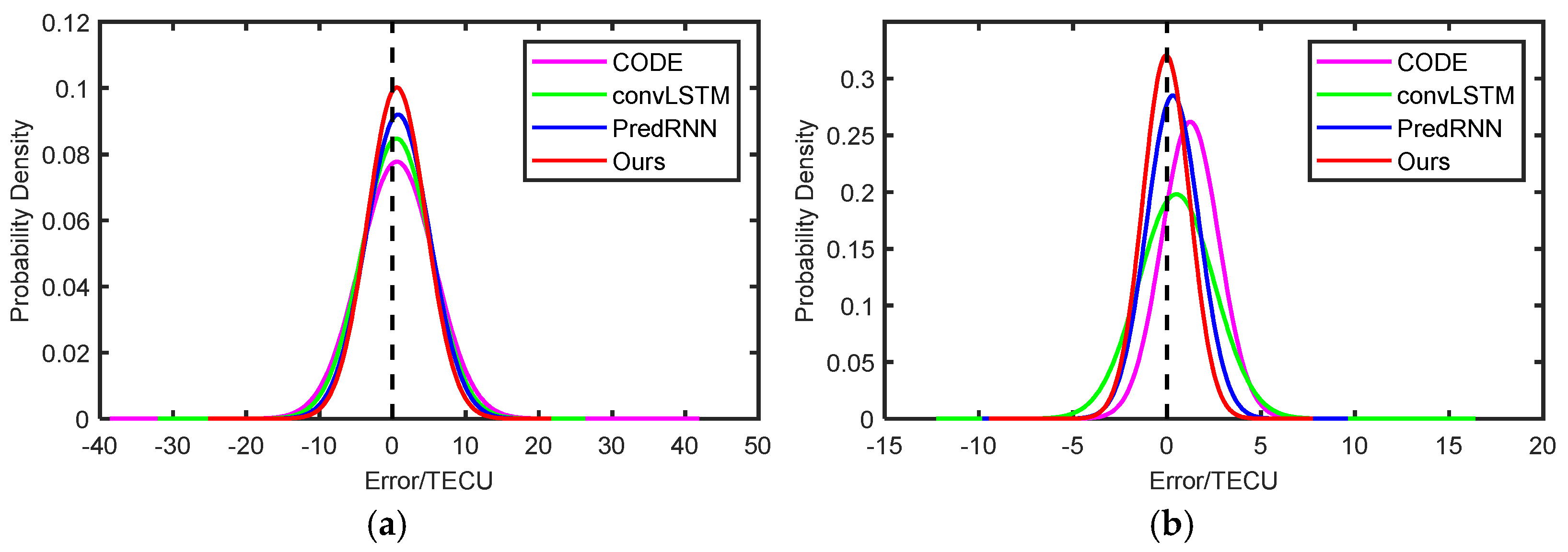
4.3.1. Comparison with IGS Final TEC Products

The final TEC product of the IGS combined had a higher accuracy than the final TEC product of the individual IAAC, and we used these as training data for the model. Therefore, we used the final TEC of the IGS, combined with internal validation data, to assess the fitting ability and forecast performance of the spatiotemporal network model.

The convLSTM model, the PredRNN model, and our proposed spatiotemporal network model were trained using the global ionospheric TEC training set that was prepared in advance. Two global ionospheric TEC test sets, for maximum and minimum solar activity, were used to test the results. We compared the global ionospheric TEC one-day forecast results of the convLSTM model, the PredRNN model, and our spatiotemporal network model. We examined the forecast accuracy of several algorithms for different solar activity conditions and different times. We demonstrated the superiority of our algorithm in modeling global ionospheric TEC compared to the other two spatiotemporal prediction algorithms.

CODE is one of the IAACs that publishes products containing global ionospheric TEC forecasts for the next day and following two days. The global ionospheric TEC maps predicted by CODE have a higher accuracy than the global ionospheric TEC maps predicted by other IAACs. Therefore, the one-day forecast data provided by CODE were used for comparison with our proposed algorithm to further validate the accuracy of the algorithm.

The quantitative evaluation results of the one-day forecasts of the four algorithms for the maximum and minimum solar activity periods are shown in

Table 1. Results of the precision evaluation of periods of maximum solar activity. TECU is a unit of ionospheric TEC, defined as containing 10¹⁶ electrons per square meter.

	$\overline{\mathbf{R}\mathbf{M}\mathbf{S}\mathbf{E}}\left(\mathbf{TECU}\right)$	$\overline{\mathbf{M}\mathbf{A}\mathbf{E}}\left(\mathbf{TECU}\right)$	$\overline{\mathbf{P}\mathbf{S}\mathbf{N}\mathbf{R}}$
CODE [20]	4.9815	3.6910	26.1758
convLSTM [40,41,42]	4.6596	3.2744	26.6119
PredRNN [43]	4.3462	3.1449	27.2195
Ours	3.9259	2.8274	28.2035

and

Table 2. Results of the precision evaluation of periods of minimum solar activity. TECU is a unit of ionospheric TEC, defined as containing 10¹⁶ electrons per square meter.

	$\overline{\mathbf{R}\mathbf{M}\mathbf{S}\mathbf{E}}\left(\mathbf{TECU}\right)$	$\overline{\mathbf{M}\mathbf{A}\mathbf{E}}\left(\mathbf{TECU}\right)$	$\overline{\mathbf{P}\mathbf{S}\mathbf{N}\mathbf{R}}$
CODE	1.9524	1.5073	24.2228
convLSTM	1.9315	1.4048	24.8503
PredRNN	1.3845	1.0126	27.5427
Ours	1.1971	0.8826	28.7954

, respectively. According to the tables, our proposed spatiotemporal network model has the best forecast accuracy among the four algorithms for both the maximum and minimum solar activity periods, with the PredRNN model coming in second and CODE being slightly less accurate. Compared to CODE’s traditional global ionospheric TEC forecasting algorithm, the three deep learning spatiotemporal sequence forecasting algorithms have better forecasting performance. They can learn the temporal variability and spatial characteristics of global ionospheric TEC at the same time, and can better fit non-linear relationships such as global ionospheric TEC’s spatiotemporal autocorrelation.

During the period of maximum solar activity, the $\overline{\mathrm{RMSE}}$ of our spatiotemporal network model forecasts improved by 21.19% compared to the one-day forecasts of CODE, 15.75% compared to the convLSTM model, and 9.67% compared to the PredRNN model. The $\overline{\mathrm{MAE}}$ of our spatiotemporal network model forecasts improved by 23.40% compared to the one-day forecasts from CODE, 13.65% compared to the convLSTM model, and 10.10% compared to the PredRNN model. The $\overline{\mathrm{PSNR}}$ of our spatiotemporal network model forecasts improved by 2.0277 compared to the one-day forecasts from CODE, 1.5916 compared to the convLSTM model, and 0.9840 compared to the PredRNN model.

During the period of minimum solar activity, the $\overline{\mathrm{RMSE}}$ of our spatiotemporal network model forecasts improved by 38.69% compared to the one-day forecasts of the CODE, 38.02% compared to the convLSTM, and 13.54% compared to the PredRNN model. The $\overline{\mathrm{MAE}}$ of our spatiotemporal network model forecasts improved by 41.44% compared to the CODE one-day forecasts, 37.17% compared to the convLSTM model forecasts, and 12.84% compared to the PredRNN model forecasts. The $\overline{\mathrm{PSNR}}$ of our spatiotemporal network model forecasts improved by 4.5726 compared to the one-day forecasts from CODE, 3.9451 compared to the convLSTM model, and 1.2527 compared to the PredRNN model.

Figure 7 shows the error distributions of the future global ionospheric TEC maps that were forecasted by the four algorithms during the maximum and minimum solar activity periods, respectively, and we compared the four algorithms two-by-two for comparison purposes. According to the statistics, during both the maximum and minimum solar activity periods, the PredRNN model forecasts are closer to the IGS TEC values than the CODE model. The forecasts of our spatiotemporal network model are closer to the IGS TEC values than the convLSTM model. Our spatiotemporal network model forecasts are also better than the PredRNN model.

During the maximum and minimum solar activity periods, Figure 8 depicts the normal distribution of the errors of the global ionospheric TEC maps forecasted by the four algorithms for the next day. The error distribution of our spatiotemporal network model was smaller and more concentrated during the maximum solar activity period. The error distribution of our spatiotemporal network model was closer to the mean value of zero during the minimum solar activity period. Overall, our algorithm has a more concentrated and smaller error distribution, as well as a higher forecast accuracy.

Figure 9 shows the global ionospheric TEC map for a randomly selected moment in time based on the four algorithms’ one-day forecast results for the period of maximum solar activity. From the subjective visualization, the global ionospheric TEC map predicted by our algorithm is most similar to the IGS’s final global ionospheric TEC map, and the TEC distribution is more consistent with the final TEC map of the IGS. In the part of the ionosphere with larger TEC values, the shape of the TEC distribution of CODE and our algorithm is more similar to the shape of the TEC distribution of the IGS. However, in terms of image brightness, the value of the TEC of our algorithm is more consistent with the value of the TEC of the IGS.

Figure 10 shows the residuals between the forecast global ionospheric TEC map presented in Figure 9 and the final global ionospheric TEC map from the IGS. It is clear from the figure that, in terms of the residual values, the differences between the global ionospheric TEC maps, the final global ionospheric TEC maps forecast by our algorithm and the final global ionospheric TEC maps from the IGS are minimal. Moreover, the magnitude of its residual values are more concentrated compared to several other algorithms and it has a higher forecast accuracy. Furthermore, when compared to several deep learning models, the CODE forecasts have larger residuals, indicating that the deep learning-based algorithm used for forecasting spatiotemporal sequences has better forecasting performance.

The global ionospheric TEC map for a randomly selected moment in time is shown in Figure 11, based on the one-day forecast results of the four algorithms for the minimum solar activity period. The global ionospheric TEC map predicted by our algorithm is the most similar to the IGS’s final global ionospheric TEC map from a subjective visual standpoint, and the TEC distribution is more consistent with the IGS’s final TEC map. The TEC values of the convLSTM model, the PredRNN model, and our proposed spatiotemporal network model are closer to the IGS TEC value in terms of image brightness. However, the shape of the TEC distribution of our algorithm is more similar to the IGS TEC distribution in the larger part of the ionospheric TEC values.

Figure 12 shows the residuals between the forecast global ionospheric TEC map presented in Figure 11 and the final global ionospheric TEC map from the IGS. It can be seen that the residuals between the forecasted global ionospheric TEC map of our proposed algorithm and the final global ionospheric TEC map of the IGS are closer to zero. Moreover, the magnitude of the residuals is more concentrated compared to the other algorithms, providing a higher forecast accuracy. In addition, as with the maximum solar activity period, the CODE forecasts for the minimum solar activity period have larger residuals compared to several deep learning models. This indicates that the deep-learning-based spatiotemporal sequence prediction algorithms have a better forecasting performance during both the maximum and minimum solar activity periods.

We further evaluated the forecast performance of the spatiotemporal network model for forecasting global ionospheric TEC changes at any point in time for a future day with a time interval of 2 h. During the maximum and minimum solar activity periods, Figure 13 shows the quantitative evaluation results for each moment of the global ionospheric TEC map for a future day with a time interval of 2 h, as forecasted by the four algorithms. During the period of maximum solar activity, our proposed algorithm has the best forecast accuracy for the first 12 h of the day, except for the second hour, which is suboptimal, and the accuracy for most of the second 12 h is suboptimal. However, it does not have the worst forecast accuracy in any case. During the minimum solar activity period, our proposed algorithm is sub-optimal for the 2nd, 4th, 16th, and 24th hours of the day, and has the best forecast accuracy for the rest of the day. Moreover, the forecast accuracy of our algorithm is higher than the one-day forecast accuracy of CODE at all times. One reason for this phenomenon may be that errors accumulate as the forecast length increases, and the spatiotemporal network model provides spurious historical time-varying properties and spatial features to the forecast results, which affects the forecast accuracy. Taken together, our algorithm shows better forecast performance with higher accuracy for the first 12 h of the day for global ionospheric TEC, during periods of both maximum and minimum solar activity.

In addition, we looked at statistics for the forecast performance of the spatiotemporal network model for 546 TEC maps on the maximum solar activity period test set, and for 546 TEC maps on the minimum solar activity period test set. As CODE, one of the IAACs provides long-term stable future day forecast data. We also compared the two full test sets with the forecast data provided by CODE to further validate the model’s accuracy, as shown in Figure 14. Over the range of two complete test sets, our method is more accurate overall, and in most cases, the forecast accuracy is better than that of CODE. In addition, the forecast accuracy of the minimum solar activity period is better than the forecast accuracy of the maximum solar activity period. The accuracy also remained relatively stable over the entire test set. At the same time, we calculated the average accuracy of the two test sets. On the maximum period solar activity test set, the average RMSE of our algorithm is 4.1407 and the average RMSE of CODE is 5.1316; the accuracy of our algorithm is improved by 19.31%. On the minimum solar activity test set, the average RMSE of our algorithm is 1.4334 and the average RMSE of CODE is 1.8115, showing an improvement of 20.87% in the accuracy of our algorithm.

In general, compared to CODE, one of the IAACs, the spatiotemporal network model can better learn the spatiotemporal characteristics of the global ionospheric TEC. It can further fit the non-linear relationships such as spatiotemporal autocorrelation. Compared to other spatiotemporal series prediction models (convLSTM and PredRNN models), the spatiotemporal network model can complement the global spatiotemporal characteristics of TEC and regional spatiotemporal characteristics. This ensures that the global spatiotemporal characteristics of global ionospheric TEC are transmitted to each other in both the temporal and spatial domains. This further suppresses the gross error and noise in the TEC data, thus effectively improving the forecast accuracy of the global ionospheric TEC.

4.3.2. Assessment Results using Altimetry Satellite VTEC

Altimeter satellites transmitting dual-frequency signals received by reflection from the ocean surface can be used to invert the VTEC in the signal propagation path [51]. This provides GNSS-independent reference data that are very useful for assessing the performance of global ionospheric TEC maps [52]. Observations from the JASON-2 and JASON-3 altimetry satellites are now commonly and internationally used to obtain VTEC. Furthermore, since the superiority of our model over other spatiotemporal series prediction models for ionospheric modeling has been verified in the previous subsection, in this subsection, we used the VTEC calculated by JASON-2/3 as external validation data. These were compared with those of CODE, which has the highest forecast accuracy in IAACs, to further validate the forecast performance of the spatiotemporal network model.

As shown in Figure 15, the bias and standard deviation (STD) of altimeter VTEC and forecast results are shown for a day that was randomly selected from the test set of maximum solar activity and minimum solar activity. Overall, during the period of maximum solar activity, the spatiotemporal network model forecasts are comparable, in terms of overall accuracy, to the one-day forecasts from CODE. For some moments, the spatiotemporal network model forecasts show better performance. During the minimum solar activity period, the accuracy of the spatiotemporal network model is slightly better than that of the one-day predictions of CODE, demonstrating good forecasting performance. The prediction performance during the period of minimum solar activity is better than that during the period of maximum solar activity, and the accuracy fluctuates less.

At the same time, as the training data for the spatiotemporal network model are the IGS final TEC, its bias and the STD from the altimeter VTEC, which should be very close to that of the IGS final TEC. Therefore, we also randomly selected nearly 1000 pieces of data to calculate the bias of the altimeter VTEC from the IGS final TEC. The bias of the IGS final TEC was compared to the similarity of the bias of the spatiotemporal network model and CODE, respectively, to assess the model fitting ability. As shown in Figure 16, the bias of the altimeter VTEC and IGS final TEC is more similar to that of the spatiotemporal network model, while the bias with CODE is significantly different. This further indicates that the forecast accuracy of the spatiotemporal network model basically meets the data accuracy of the IGS final TEC, and the model has a good fitting ability.

In addition, the most intense magnetic storm of the 24th solar cycle occurred on 17 March 2015 [53]. To verify the forecast performance of the spatiotemporal network model under severely perturbed conditions, and the generalization capability of the model, we used the spatiotemporal network model to forecast the ionospheric variability on 17 March 2015 outside the dataset. This was compared with the forecast data from CODE, which has the highest forecast accuracy in ICCAs. The bias and STD between them and the VTEC of Jason-2 were calculated separately, and the results are shown in Figure 17. Although severely affected by intense solar storms, our spatiotemporal network model still has a comparable forecast accuracy to that of CODE, is generally stable and showed some generalization ability.

Overall, compared to the altimeter VTEC data, we are limited by the accuracy of the IGS final TEC when using only the IGS final TEC as model training data. The spatiotemporal network model still achieves a forecast accuracy that is comparable to, or even slightly better than, that of CODE’s direct use of GNSS observations, effectively illustrating the forecast performance and superiority of our method. At the same time, the bias of the spatiotemporal network model is very similar to that of the final IGS TEC, indicating that the spatiotemporal network model has a good data-fitting ability. In addition, the spatiotemporal network model still shows a good forecasting performance with good robustness and some generalization ability under severe perturbation by solar storms.

In summary, our proposed spatiotemporal network model has an excellent forecasting performance when validating accuracy using in-house data (IGS final TEC). It showed an ability to significantly outperform CODE and other spatiotemporal sequence forecasting models (convLSTM model and PredRNN model), with some advantages. When using external data (altimeter VTEC) to verify accuracy, the spatiotemporal network model still performs well, achieving an accuracy close to that of the IGS final TEC. It also shows a better forecasting performance than CODE during the minimum solar activity period.

5. Conclusions

We used the ST-LSTM unit to learn the time-varying characteristics and spatial features of global ionospheric TEC. We also built two modules for global spatiotemporal characteristics extraction using the forwarding spatiotemporal characteristics transfer and regional spatiotemporal characteristics correction, via reverse spatiotemporal characteristics transfer, to construct a global ionospheric TEC spatiotemporal network model. This can compensate for the deficiencies in the spatiotemporal characteristics of the low-layer ST-LSTM units, and realize the complementarity of the TEC’s global spatiotemporal characteristics and regional spatiotemporal characteristics. This ensures that the global spatiotemporal characteristics of global ionospheric TEC are simultaneously transmitted to each other in the temporal and spatial domains. It can fit non-linear relations such as the spatiotemporal autocorrelation of TEC to forecast global ionospheric TEC. To address the non-linear, non-smooth, and highly noisy characteristics of global ionospheric TEC data, we used the Huber loss function to constrain the training process of the spatiotemporal network model, to suppress the gross error and noise in global ionospheric TEC data. This further improves the global ionospheric TEC forecast accuracy. Furthermore, our proposed algorithm can build a more accurate global ionospheric TEC forecast model using only the global ionospheric TEC map and without other parameters such as the geomagnetic index.

Our proposed algorithm was used to forecast the future one-day variation in global ionospheric TEC at various times and under various solar activity conditions. Its performance is assessed by comparing it to CODE’s one-day forecast data, the convLSTM model’s one-day forecast results, and the PredRNN model’s one-day forecast results. Under internal accuracy verification conditions, using the results of the quantitative analysis, the average RMSE, average MAE, and average PSNR of our algorithm all improved to different degrees. Compared with the CODE, convLSTM, and PredRNN models, the average RMSE of our algorithm improved by 21.19, 15.75, and 9.67%, respectively, during the maximum solar activity period. The average RMSE of our algorithm improved by 38.69, 38.02, and 13.54%, respectively, during the minimum solar activity period. From the visual analysis, our algorithm’s global ionospheric TEC distribution forecast was shown to be more consistent with the IGS’s final TEC distribution. Evaluating the global ionospheric TEC forecasts individually for each moment of the time interval of 2 h, our algorithm showed a higher forecast accuracy in the first 12 h of the day and is more suitable for short-term forecasts of up to 12 h than several other algorithms. For the whole dataset, our algorithm has a higher overall forecast accuracy than CODE. Under external accuracy verification conditions, the accuracy of our algorithm is very similar to that of the final IGS TEC. The forecast performance is similar to that of CODE during periods of maximum solar activity, and better than that of CODE during periods of minimum solar activity. Overall, our proposed method can further improve global ionospheric TEC forecast accuracy and be used to correct ionospheric delay error in satellite navigation positioning.

In addition, real-time data are crucial in satellite navigation positioning, but our algorithm uses the final TEC of the IGS for the study, which has a delay of about 11 days and lacks real-time data. The forecast performance of our algorithm is limited by the accuracy of the IGS final TEC. Therefore, in future work, we intend to realize the real-time forecasting of global ionospheric TEC, considering the use of GNSS real-time data to reduce accuracy constraints. Further studies on the spatial and temporal properties of global ionospheric TEC will be carried out to improve the forecast duration while maintaining forecast accuracy.

References

1. Song, R.; Zhang, X.M.; Zhou, C.; Liu, J.; He, J.H. Predicting TEC in China based on the neural networks optimized by genetic algorithm. Adv. Space Res. 2018, 62, 745–759. [Google Scholar] [CrossRef]
2. Qiu, F.Q.; Pan, X.; Luo, X.M.; Lai, Z.L.; Jiang, K.; Wang, G.X. Global ionospheric TEC prediction model integrated with semiparametric kernel estimation and autoregressive compensation. Chin. J. Geophys. Chin. Ed. 2021, 64, 3021–3029. [Google Scholar]
3. Inyurt, S.; Razin, M.R.G. Regional application of ANFIS in ionosphere time series prediction at severe solar activity period. Acta Astronaut. 2021, 179, 450–461. [Google Scholar] [CrossRef]
4. Bilitza, D. International reference ionosphere: Recent developments. Radio Sci. 1986, 21, 343–346. [Google Scholar] [CrossRef]
5. Bent, R.B.; Llewellyn, S.K.; Nesterczuk, G.; Schmid, P.E. The development of a highly-successful worldwide empirical ionospheric model and its use in certain aspects of space communications and worldwide total electron content investigations. In Effect of the Ionosphere on Space Systems and Communications; U.S. Government Printing Office: Washington, DC, USA, 1975; pp. 13–28. [Google Scholar]
6. Klobuchar, J.A. Ionospheric time-delay algorithm for single-frequency GPS users. IEEE Trans. Aerosp. Electron. Syst. 1987, 3, 325–331. [Google Scholar] [CrossRef]
7. Nava, B.; Coisson, P.; Radicella, S.M. A new version of the NeQuick ionosphere electron density model. J. Atmos. Sol. Terr. Phys. 2008, 70, 1856–1862. [Google Scholar] [CrossRef]
8. Jiang, H.; Liu, J.; Wang, Z.; An, J.; Ou, J.; Liu, S.; Wang, N. Assessment of spatial and temporal TEC variations derived from ionospheric models over the polar regions. J. Geod. 2019, 93, 455–471. [Google Scholar] [CrossRef]
9. Holt, J.M.; Zhang, S.-R.; Buonsanto, M.J. Regional and local ionospheric models based on Millstone Hill incoherent scatter radar data. Geophys. Res. Lett. 2002, 29, 48-1–48-3. [Google Scholar] [CrossRef]
10. Kouris, S.; Fodadis, D.; Zolesi, B. Specifications of the F-region variations for quiet and disturbed conditions. Phys. Chem. Earth C Sol. Terr. Planet. Sci. 1999, 24, 321–327. [Google Scholar] [CrossRef]
11. Aa, E.; Huang, W.; Yu, S.; Liu, S.; Shi, L.; Gong, J.; Chen, Y.; Shen, H. A regional ionospheric TEC mapping technique over China and adjacent areas on the basis of data assimilation. J. Geophys. Res. Space Phys. 2015, 120, 5049–5061. [Google Scholar] [CrossRef] [Green Version]
12. Mandrikova, O.V.; Fetisova, N.V.; Al-Kasasbeh, R.T.; Klionskiy, D.M.; Geppener, V.V.; Ilyash, M.Y. Ionospheric parameter modelling and anomaly discovery by combining the wavelet transform with autoregressive models. Ann. Geophys. 2015, 58, 550. [Google Scholar]
13. Ratnam, D.V.; Otsuka, Y.; Sivavaraprasad, G.; Dabbakuti, J.K. Development of multivariate ionospheric TEC forecasting algorithm using linear time series model and ARMA over low-latitude GNSS station. Adv. Space Res. 2019, 63, 2848–2856. [Google Scholar] [CrossRef]
14. Kaselimi, M.; Voulodimos, A.; Doulamis, N.; Doulamis, A.; Delikaraoglou, D. Deep recurrent neural networks for ionospheric variations estimation using gnss measurements. IEEE Trans. Geosci. Remote Sens. 2021, 60, 3090856. [Google Scholar] [CrossRef]
15. An, X.; Meng, X.; Chen, H.; Jiang, W.; Xi, R.; Chen, Q. Modelling Global Ionosphere Based on Multi-Frequency, Multi-Constellation GNSS Observations and IRI Model. Remote Sens. 2020, 12, 439. [Google Scholar] [CrossRef] [Green Version]
16. Krypiak-Gregorczyk, A.; Wielgosz, P.; Borkowski, A. Ionosphere model for European region based on multi-GNSS data and TPS interpolation. Remote Sens. 2017, 9, 1221. [Google Scholar] [CrossRef] [Green Version]
17. Wang, J.; Huang, G.; Zhou, P.; Yang, Y.; Zhang, Q.; Gao, Y. Advantages of Uncombined Precise Point Positioning with Fixed Ambiguity Resolution for Slant Total Electron Content (STEC) and Differential Code Bias (DCB) Estimation. Remote Sens. 2020, 12, 304. [Google Scholar] [CrossRef] [Green Version]
18. Ren, X.; Zhang, X.; Xie, W.; Zhang, K.; Yuan, Y.; Li, X. Global ionospheric modelling using multi-GNSS: BeiDou, Galileo, GLONASS and GPS. Sci. Rep. 2016, 6, 33499. [Google Scholar] [CrossRef] [Green Version]
19. Zhao, J.; Hernández-Pajares, M.; Li, Z.; Wang, N.; Yuan, H. Integrity investigation of global ionospheric TEC maps for high-precision positioning. J. Geod. 2021, 95, 35. [Google Scholar] [CrossRef]
20. Schaer, S. Mapping and Predicting the Earth’s Ionosphere Using the Global Positioning System; Institut für Geodäsie und Photogrammetrie, Eidg. Technische Hochschule Zürich: Zürich, Switzerland, 1999. [Google Scholar]
21. García-Rigo, A.; Monte, E.; Hernández-Pajares, M.; Juan, J.; Sanz, J.; Aragón-Angel, A.; Salazar, D. Global prediction of the vertical total electron content of the ionosphere based on GPS data. Radio Sci. 2011, 46, 1–3. [Google Scholar] [CrossRef] [Green Version]
22. Li, M.; Yuan, Y.; Wang, N.; Li, Z.; Huo, X. Performance of various predicted GNSS global ionospheric maps relative to GPS and JASON TEC data. GPS Solut. 2018, 22, 55. [Google Scholar] [CrossRef]
23. Zhang, G.P. Time series forecasting using a hybrid ARIMA and neural network model. Neurocomputing 2003, 50, 159–175. [Google Scholar] [CrossRef]
24. Sabzehee, F.; Farzaneh, S.; Sharifi, M.A.; Akhoondzadeh, M. TEC Regional Modeling and prediction using ANN method and single frequency receiver over IRAN. Ann. Geophys. 2018, 61, 103. [Google Scholar] [CrossRef] [Green Version]
25. Habarulema, J.B.; McKinnell, L.A.; Cilliers, P.J.; Opperman, B.D. Application of Neural Networks to South African GPS TEC Modelling. Adv. Space Res. 2009, 43, 1711–1720. [Google Scholar] [CrossRef]
26. Tebabal, A.; Radicella, S.; Damtie, B.; Migoya-Orue, Y.; Nigussie, M.; Nava, B. Feed forward neural network based ionospheric model for the East African region. J. Atmos. Sol. Terr. Phys. 2019, 191, 105052. [Google Scholar] [CrossRef]
27. Adolfs, M.; Hoque, M.M. A Neural Network-Based TEC Model Capable of Reproducing Nighttime Winter Anomaly. Remote Sens. 2021, 13, 4559. [Google Scholar] [CrossRef]
28. Huang, Z.; Yuan, H. Ionospheric single-station TEC short-term forecast using RBF neural network. Radio Sci. 2014, 49, 283–292. [Google Scholar] [CrossRef]
29. Zhang, Z.; Pan, S.; Gao, C.; Zhao, T.; Gao, W. Support vector machine for regional ionospheric delay modeling. Sensors 2019, 19, 2947. [Google Scholar] [CrossRef] [Green Version]
30. Zhukov, A.V.; Yasyukevich, Y.V.; Bykov, A.E. GIMLi: Global Ionospheric total electron content model based on machine learning. GPS Solut. 2021, 25, 19. [Google Scholar] [CrossRef]
31. Voulodimos, A.; Doulamis, N.; Doulamis, A.; Protopapadakis, E. Deep learning for computer vision: A brief review. Comput. Intell. Neurosci. 2018, 2018, 7068349. [Google Scholar] [CrossRef]
32. Liu, B.; Wang, M.; Li, Y.; Chen, H.; Li, J. Deep Learning for Spatio-Temporal Sequence Forecasting:A Survey. J. Beijing Univ. Technol. 2021, 47, 925–941. [Google Scholar]
33. Hochreiter, S.; Schmidhuber, J. Long short-term memory. Neural Comput. 1997, 9, 1735–1780. [Google Scholar] [CrossRef] [PubMed]
34. Kaselimi, M.; Voulodimos, A.; Doulamis, N.; Doulamis, A.; Delikaraoglou, D.J.R.S. A Causal Long Short-Term Memory Sequence to Sequence Model for TEC Prediction Using GNSS Observations. Remote Sens. 2020, 12, 1354. [Google Scholar] [CrossRef]
35. Liu, L.; Zou, S.; Yao, Y.; Wang, Z.J.S.W. Forecasting global ionospheric TEC using deep learning approach. Space Weather 2020, 18, e2020SW002501. [Google Scholar] [CrossRef]
36. Sun, W.; Xu, L.; Huang, X.; Zhang, W.; Yuan, T.; Chen, Z.; Yan, Y. Forecasting of ionospheric vertical total electron content (TEC) using LSTM networks. In Proceedings of the 2017 International Conference on Machine Learning and Cybernetics (ICMLC), Ningbo, China, 9–12 July 2017; pp. 340–344. [Google Scholar]
37. Xiong, P.; Zhai, D.; Long, C.; Zhou, H.; Zhang, X.; Shen, X.J.S.W. Long Short-Term Memory Neural Network for Ionospheric Total Electron Content Forecasting Over China. Space Weather 2021, 19, e2020SW002706. [Google Scholar] [CrossRef]
38. Chen, Z.; Jin, M.; Deng, Y.; Wang, J.S.; Huang, H.; Deng, X.; Huang, C.M. Improvement of a deep learning algorithm for total electron content maps: Image completion. J. Geophys. Res. Space Phys. 2019, 124, 790–800. [Google Scholar] [CrossRef] [Green Version]
39. Lee, S.; Ji, E.Y.; Moon, Y.J.; Park, E. One-Day Forecasting of Global TEC Using a Novel Deep Learning Model. Space Weather 2021, 19, 2020SW002600. [Google Scholar] [CrossRef]
40. Xingjian, S.; Chen, Z.; Wang, H.; Yeung, D.-Y.; Wong, W.-K.; Woo, W.-C. Convolutional LSTM network: A machine learning approach for precipitation nowcasting. Adv. Neural Inf. Process. Syst. 2015, 28, 802–810. [Google Scholar]
41. Liu, L.; Morton, Y.J.; Liu, Y. Machine Learning Prediction of Storm-Time High-Latitude Ionospheric Irregularities From GNSS-Derived ROTI Maps. Geophys. Res. Lett. 2021, 48, e2021GL095561. [Google Scholar] [CrossRef]
42. Zhang, F.; Zhou, C.; Wang, C.; Zhao, J.; Liu, Y.; Xia, G.; Zhao, Z. Global ionospheric TEC prediction based on deep learning. Chin. J. Radio Sci. 2021, 36, 553–561. [Google Scholar]
43. Wang, Y.; Long, M.; Wang, J.; Gao, Z.; Yu, P.S. Predrnn: Recurrent neural networks for predictive learning using spatiotemporal lstms. In Proceedings of the 31st International Conference on Neural Information Processing Systems, Long Beach, CA, USA, 4–9 December 2017; pp. 879–888. [Google Scholar]
44. Lu, T.; Huang, J.; He, X.; Lv, Y. Short-Term Ionospheric TEC Prediction Using EWT-Elman Combination Model. J. Geod. Geodyn. 2021, 41, 666–671. [Google Scholar]
45. Huber, P.J. Robust estimation of a location parameter. In Breakthroughs in Statistics; Springer: New York, NY, USA, 1992; pp. 492–518. [Google Scholar]
46. Roma-Dollase, D.; Hernández-Pajares, M.; Krankowski, A.; Kotulak, K.; Ghoddousi-Fard, R.; Yuan, Y.; Li, Z.; Zhang, H.; Shi, C.; Wang, C. Consistency of seven different GNSS global ionospheric mapping techniques during one solar cycle. J. Geod. 2018, 92, 691–706. [Google Scholar] [CrossRef] [Green Version]
47. Hernández-Pajares, M.; Juan, J.M.; Sanz, J.; Orus, R.; Garcia-Rigo, A.; Feltens, J.; Komjathy, A.; Schaer, S.C.; Krankowski, A. The IGS VTEC maps: A reliable source of ionospheric information since 1998. J. Geod. 2009, 83, 263–275. [Google Scholar] [CrossRef]
48. Rauch, H.E.; Tung, F.; Striebel, C.T. Maximum likelihood estimates of linear dynamic systems. AIAA J. 1965, 3, 1445–1450. [Google Scholar] [CrossRef]
49. Zhang, Y.; Yin, C.; Wu, Q.; He, Q.; Zhu, H. Location-Aware Deep Collaborative Filtering for Service Recommendation. IEEE Trans. Syst. Man Cybern. Syst. 2021, 51, 3796–3807. [Google Scholar] [CrossRef]
50. Mangasarian, O.L.; Musicant, D.R. Robust linear and support vector regression. IEEE Trans. Pattern Anal. Mach. Intell. 2000, 22, 950–955. [Google Scholar] [CrossRef]
51. Hernández-Pajares, M. IGS Ionosphere WG Status Report: Performance of IGS Ionosphere TEC Maps-Position Paper; IGS Workshop: Bern, Switzerland, 2004. [Google Scholar]
52. Hernández-Pajares, M.; Roma-Dollase, D.; Krankowski, A.; García-Rigo, A.; Orús-Pérez, R. Methodology and consistency of slant and vertical assessments for ionospheric electron content models. J. Geod. 2017, 91, 1405–1414. [Google Scholar] [CrossRef]
53. Jin, S.; Jin, R.; Kutoglu, H. Positive and negative ionospheric responses to the March 2015 geomagnetic storm from BDS observations. J. Geod. 2017, 91, 613–626. [Google Scholar] [CrossRef]
Figure 1. The distribution of global IGS stations, the orange dots indicate IGS observatories at various locations around the world.
Remotesensing 14 01717 g001
Figure 2. A standard global ionospheric TEC map. Shown here is the global distribution of ionospheric TEC at hour 8 on 3 January 2013.
Remotesensing 14 01717 g002
Figure 3. The ST-LSTM unit’s internal structure. Superscript l indicates the number layer of the ST-LSTM unit in the stack, and subscript t indicates the current moment. Different letters indicate different parameters in the ST-LSTM unit.
Remotesensing 14 01717 g003
Figure 4. Spatiotemporal Network Model structure. Letters without the ~ symbol indicate the output of the global spatiotemporal characteristics extraction part, and letters with the ~ symbol indicate the output of the regional spatiotemporal characteristics correction part. The red arrow shows the ionospheric global spatiotemporal characteristics extraction module. The blue arrow shows the ionospheric regional spatiotemporal characteristics correction module.
Remotesensing 14 01717 g004
Figure 5. Structure of the ST-LSTM unit for the modified region spatiotemporal properties module. Different letters indicate different parameters in the ST-LSTM unit, superscript l indicates the number layer of the ST-LSTM unit in the stack and subscript t indicates the current moment.
Remotesensing 14 01717 g005
Figure 6. The convergence performance of the spatiotemporal network model using Huber loss function, L1 loss function, and L2 loss function trained for 200 epochs, respectively.
Remotesensing 14 01717 g006
Figure 7. Global ionospheric TEC map error distribution statistics for the maximum and minimum solar activity period forecasts. (a,b) are the error distribution statistics of the CODE and PredRNN models’ prediction results for the maximum and minimum solar activity periods, respectively. (c,d) are the error distribution statistics of the convLSTM and our models’ prediction results for the maximum and minimum solar activity periods, respectively. (e,f) are the error distribution statistics of the PredRNN models’ and our models’ prediction results for the maximum and minimum solar activity periods, respectively.
Remotesensing 14 01717 g007
Figure 8. Normal distribution of errors in global ionospheric TEC maps for the maximum and minimum solar activity period forecasts. (a) is a plot of the normal distribution of errors in the results of four algorithms for forecasting periods of maximum solar activity. (b) is a plot of the normal distribution of errors in the results of four algorithms for forecasting periods of minimum solar activity.
Remotesensing 14 01717 g008
Figure 9. Global ionospheric TEC map during periods of maximum solar activity. (ad) are the global ionospheric TEC maps forecast by CODE, the convLSTM model, the PredRNN model, and our spatiotemporal network model, respectively. (e) is the final global ionospheric TEC map from the IGS.
Remotesensing 14 01717 g009
Figure 10. Global ionospheric TEC map residuals during periods of maximum solar activity. (a) is the residual of the global ionospheric TEC map forecast by CODE. (b) is the residual of the global ionospheric TEC map forecast by convLSTM model. (c) is the residual of the global ionospheric TEC map forecast by PredRNN model. (d) is the residual of the global ionospheric TEC map forecast by our spatiotemporal network model.
Remotesensing 14 01717 g010
Figure 11. Global ionospheric TEC map during periods of minimum solar activity. (ad) are the global ionospheric TEC maps forecast by CODE, the convLSTM model, the PredRNN model, and our spatiotemporal network model, respectively. (e) is the final global ionospheric TEC map from the IGS.
Remotesensing 14 01717 g011
Figure 12. Global ionospheric TEC map residuals during periods of minimum solar activity. (a) is the residual of the global ionospheric TEC map forecast by CODE. (b) is the residual of the global ionospheric TEC map forecast by convLSTM model. (c) is the residual of the global ionospheric TEC map forecast by PredRNN model. (d) is the residual of the global ionospheric TEC map forecast by our spatiotemporal network model.
Remotesensing 14 01717 g012aRemotesensing 14 01717 g012b
Figure 13. Accuracy assessment for each moment of the day during the maximum and minimum periods of solar activity. (a) is the average PSNR of the four algorithms during periods of maximum solar activity. (b) is the average PSNR of the four algorithms during periods of minimum solar activity. (c) is the average MAE of the four algorithms during periods of maximum solar activity. (d) is the average MAE of the four algorithms during periods of minimum solar activity. (e) is the average PSNR of the four algorithms during periods of maximum solar activity. (f) is the average PSNR of the four algorithms during periods of minimum solar activity.
Remotesensing 14 01717 g013aRemotesensing 14 01717 g013b
Figure 14. Accuracy assessment of the maximum solar activity period test set and the minimum solar activity period test set. (a) shows the accuracy of 546 global ionospheric TEC maps from the maximum solar activity test set. (b) shows the accuracy of 546 global ionospheric TEC maps on the minimum solar activity test set.
Remotesensing 14 01717 g014aRemotesensing 14 01717 g014b
Figure 15. The accuracy of the maximum solar activity and minimum solar activity test sets was assessed using Jason-2/3 VTEC. (a) is the bias between the altimeter VTEC and the forecast for the maximum solar activity. (b) is the STD of the difference between the altimeter VTEC and the forecast for the maximum solar activity. (c) is the bias between the altimeter VTEC and the forecast for the period of minimum solar activity. (d) is the STD of the difference between the altimeter VTEC and the forecast for the period of minimum solar activity.
Remotesensing 14 01717 g015
Figure 16. The bias of the forecast data compared to the IGS final TEC bias. (a) is a comparison of the bias between the altimeter VTEC and CODE with the bias between the altimeter VTEC and the IGS final TEC. (b) is a comparison of the bias between the altimeter VTEC and our algorithm with the bias between the altimeter VTEC and the IGS final TEC.
Remotesensing 14 01717 g016
Figure 17. Accuracy assessment under extreme magnetic storm conditions on 17 March 2015. (a) is the bias between the altimeter VTEC and the forecast results. (b) is the STD of the difference between the altimeter VTEC and the forecast results.
Remotesensing 14 01717 g017