
Heterogeneous Urban Thermal Contribution of Functional Construction Land Zones: A Case Study in Shenzhen, China


Abstract
:
1. Introduction
2. Materials and Methods
2.1. Study Area
2.2. Data Sources
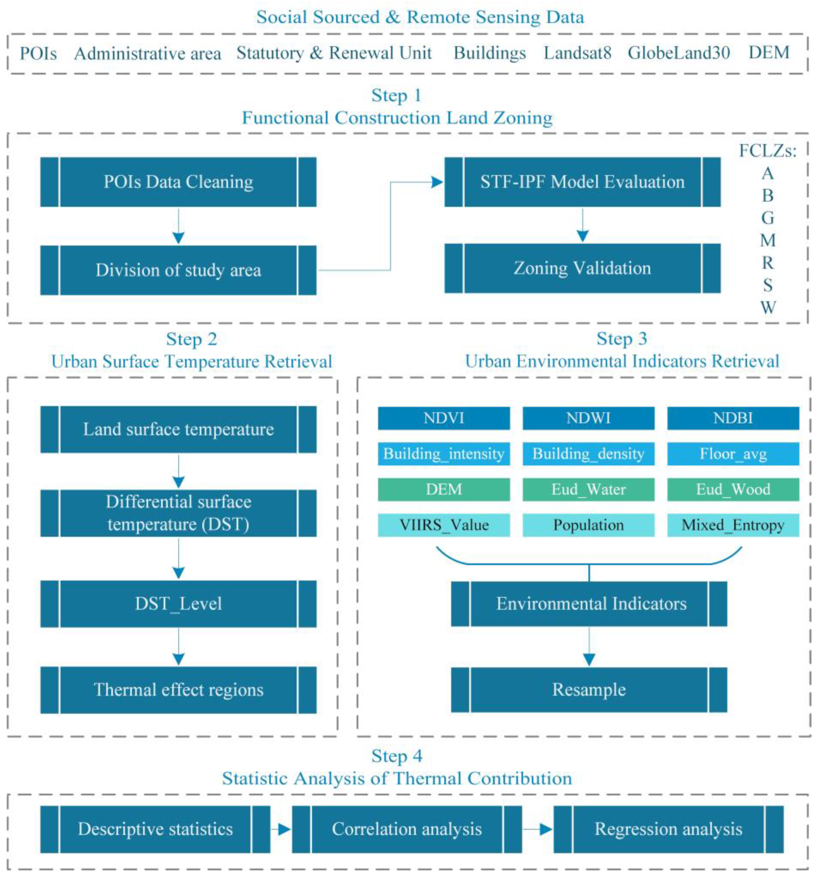
2.3. Methods
2.3.1. Functional Construction Land Zoning
- Division of study area
- 2.
- Matching POIs attributions to functional construction land zones
- 3.
- Calculation of POIs representativeness in patches
- 4.
- Recognition vectors evaluation
2.3.2. Urban Surface Temperature Retrieval
2.3.3. Urban Environmental Indicators Retrieval
- 5.
- Biophysical indicators
- 6.
- Building indicators
- 7.
- Location and social-economic indicators
2.3.4. Statistical Analysis
3. Results
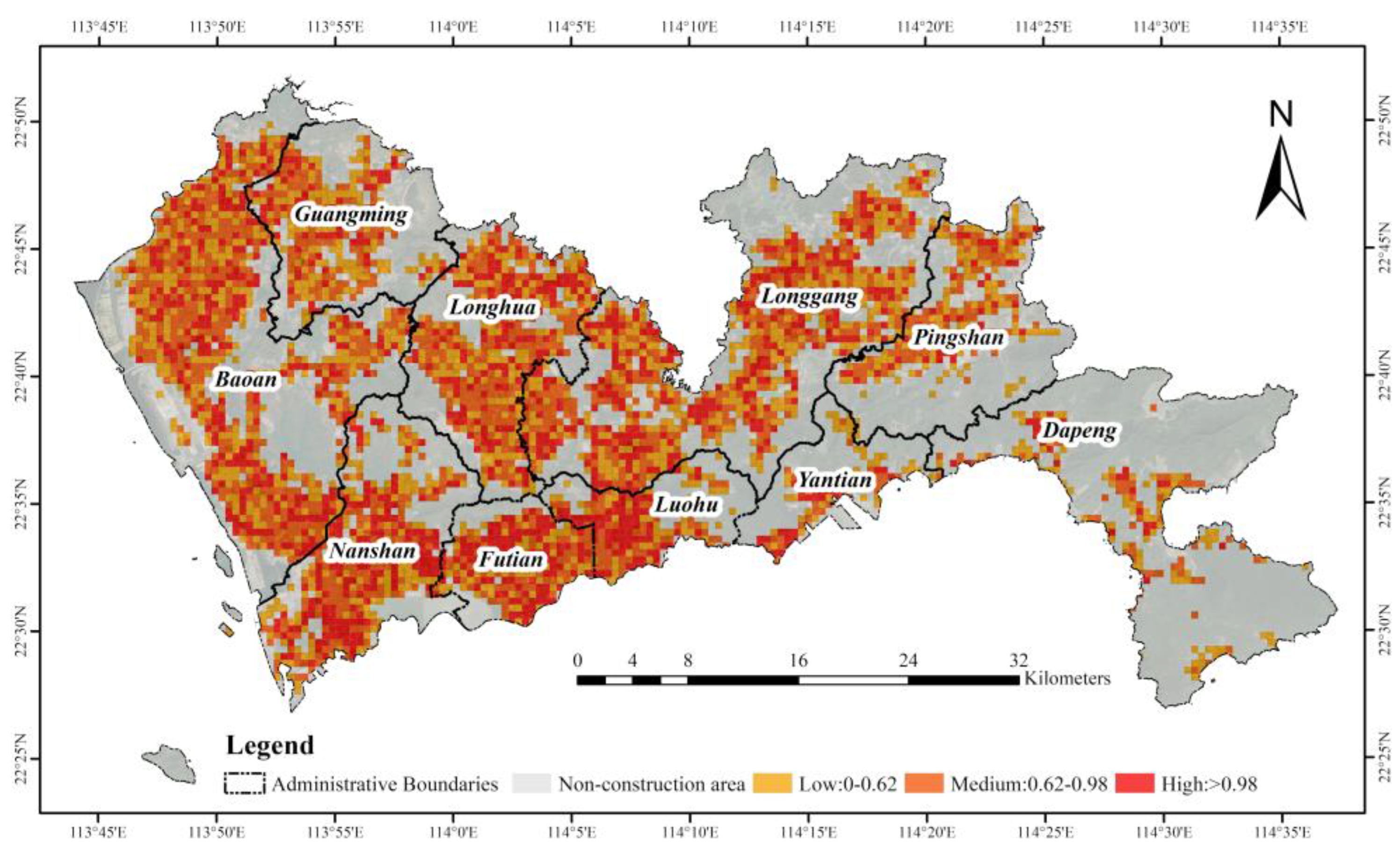
3.1. Mapping of FCLZs
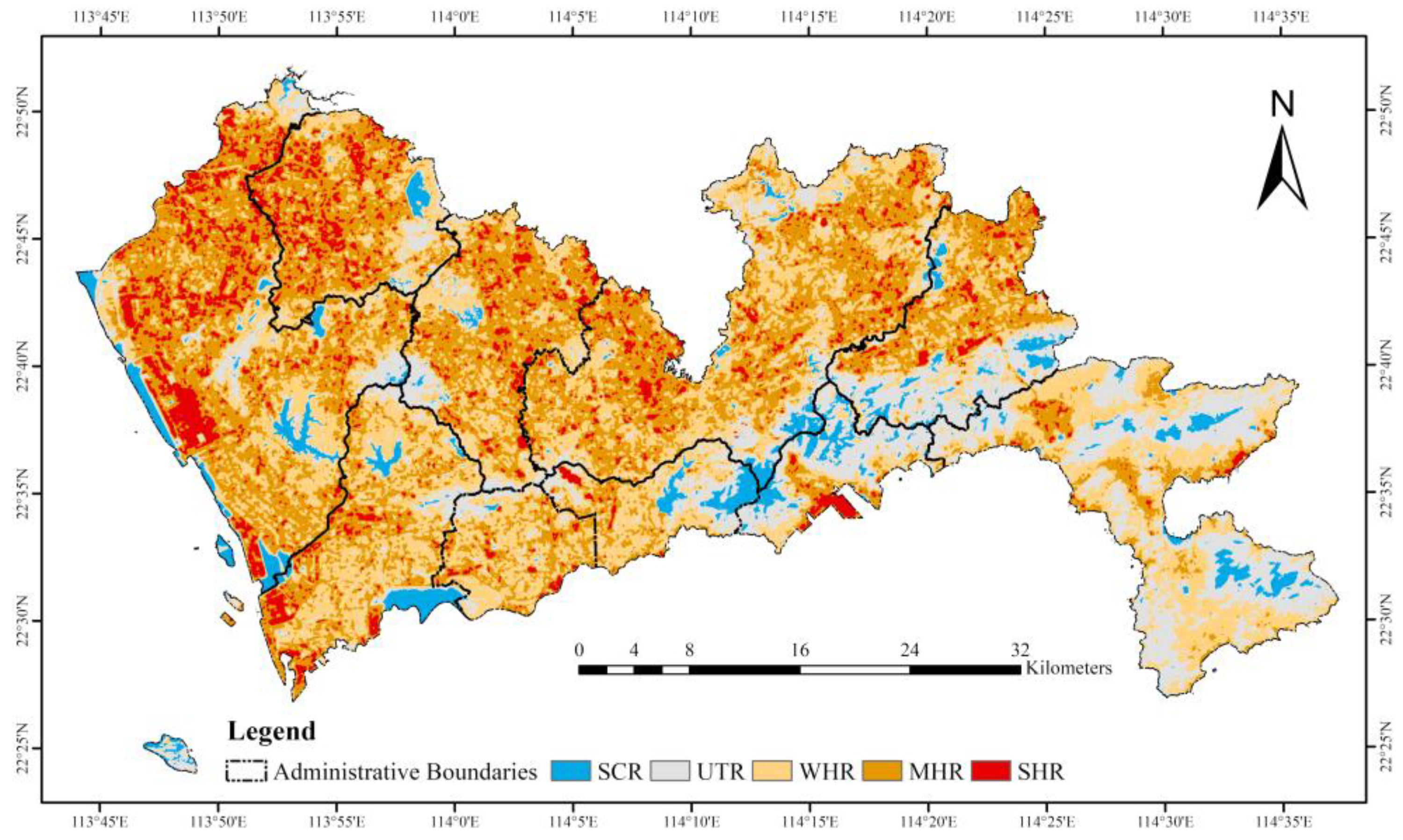
3.2. Differential Surface Temperature in FCLZs
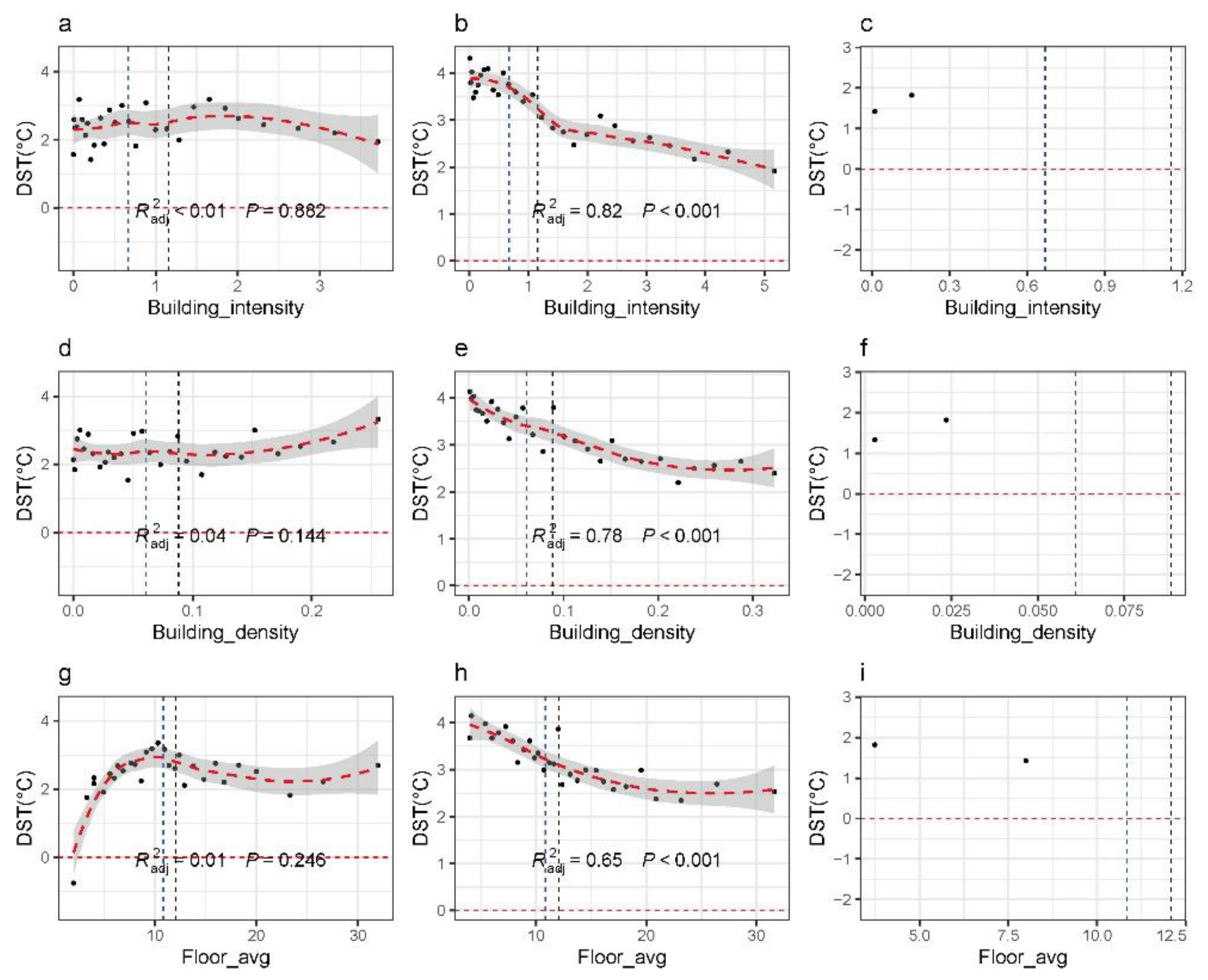
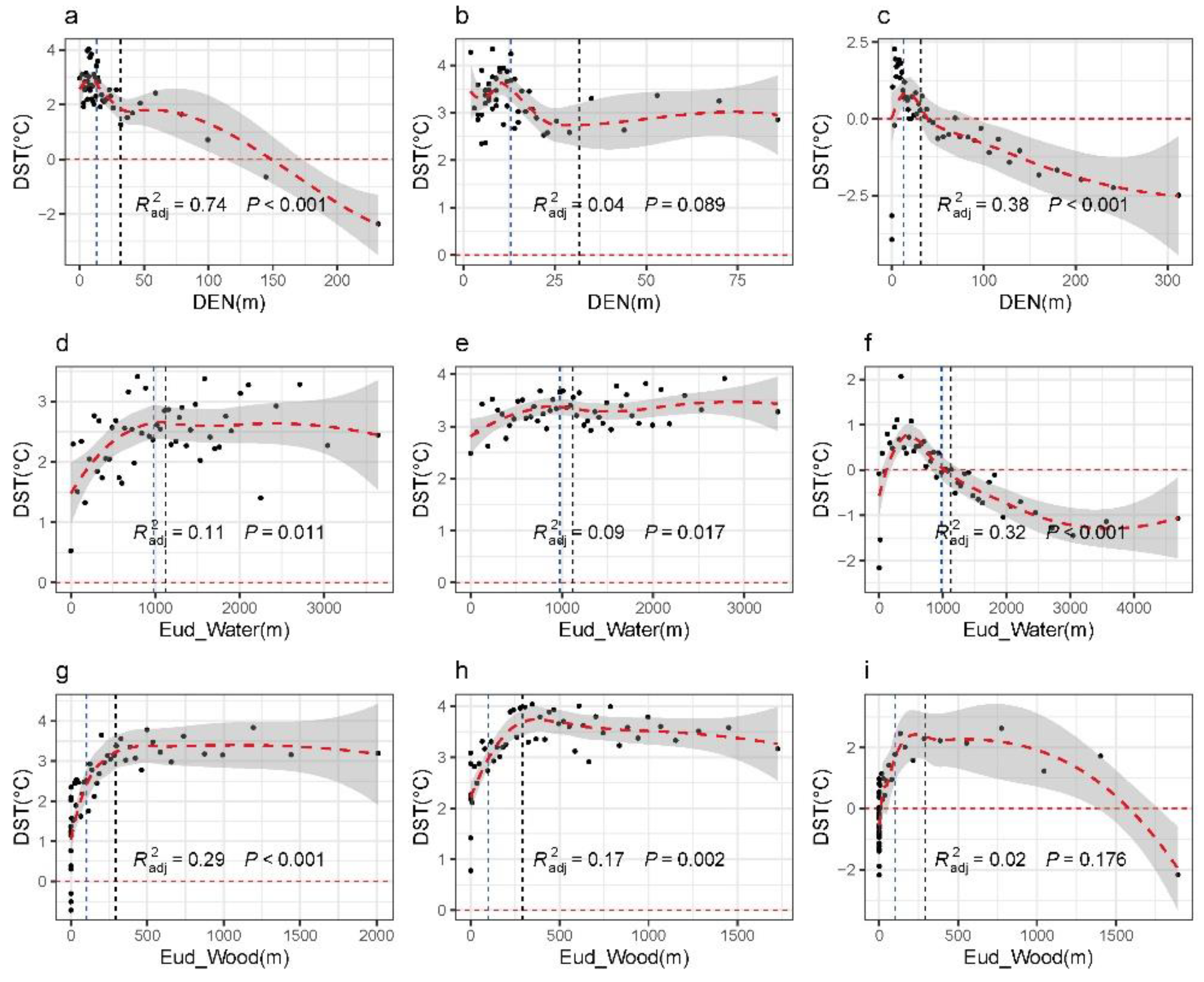
3.3. DST Relationships with Surface Environmental Indictors
4. Discussion
4.1. Consistency Analysis of Recognized FCLZs
4.2. Differential Thermal Contribution in FCLZs
4.3. Differential Responses of DST to Environmental Indicators
4.4. Potential Implication and Future Directions
5. Conclusions
Author Contributions
Funding
Conflicts of Interest
Appendix A

| Functional Class | Sub-Functional Class | Class Code | Tag of POIs |
|---|---|---|---|
| Residential Function | --- | R | Residential community, villas, community centers |
| Administration and public services Function | Administration | A1 | Government agency, Industrial and commercial bureau, public security bureau, procuratorates, courts, democratic Parties, social organization, public institutions |
| Cultural facilities | A2 | Public library, museum, science, and technology museum, art gallery, archives center, exhibition center, convention center | |
| Education and research development | A3 | Colleges and universities, technical secondary school, high school, middle school, primary school, research, and development institution | |
| Sports | A4 | Gymnasium, court, sports training sites | |
| Medical Treatment and Public Health | A5 | Health care services, general hospital, specialized hospital, clinic, emergency center, disease prevention agency | |
| Public welfare | A6 | Welfare house, nursing home, orphanage | |
| Conservation of historic landmarks and sites | A7 | Scenic spots and historical sites, tourist attractions, revolutionary site | |
| Religious facilities | A9 | Church, mosque, temple | |
| Business Services Function (B) | Commercial Facilities | B1 | Retail business (shopping malls, supermarkets, shops, etc.) |
| Wholesale market | |||
| Catering services (restaurant, bar, tea house, cake shop, cafe, cold drink, and dessert shop) | |||
| Accommodation services (hotels, guest houses, and resorts) | |||
| Business Facilities | B2 | Financial insurance (banking and insurance company, ATM, securities company, financial and insurance service organization) | |
| Art Media (Media organizations such as music, fine arts, film, television, advertising, network media, art groups) | |||
| Other business facilities companies | |||
| Recreation facilities | B3 | Entertainment facilities (theatre, concert hall, cinema, song, dance hall, Internet cafe, amusement park) | |
| Recreation and Sports facilities (Golf Driving Range Racecourse Skating Rink Skydiving Range Motorcycle Range Shooting Range) | |||
| Public utilities | B4 | Refueling and filling stations (refueling and filling stations and other energy stations) | |
| Public facilities business outlets (telecommunications, postal service, water supply, gas supply, heat supply, etc.) | |||
| Others | B9 | Scientific, educational and cultural services (training institutions) medical and health services (clinics, medical and health sales shops, animal medical places) automobile services life services funeral services | |
| Green spaces and squares (G) | park green space | G1 | Park, zoo, botanical garden |
| street and square green area | G3 | City square | |
| Street and transport function (S) | Transport hub | S3 | Railway station, long distance bus station, port and pier |
| Transport stations | S4 | Transport facilities (car parks, bus stops, MTR stations) | |
| Others | S9 | Car training ground | |
| Manufacture Function (M) | -- | -- | Industrial park, factory |
| Warehousing and logistics Function (W) | -- | -- | Logistics warehouse |

References
- Kalnay, E.; Cai, M. Impact of urbanization and land-use change on climate. Nature 2003, 423, 528–531. [Google Scholar] [CrossRef] [PubMed]
- Deng, J.S.; Wang, K.; Hong, Y.; Qi, J.G. Spatio-temporal dynamics and evolution of land use change and landscape pattern in response to rapid urbanization. Landsc. Urban Plan. 2009, 92, 187–198. [Google Scholar] [CrossRef]
- Sun, L.; Chen, J.; Li, Q.; Huang, D. Dramatic uneven urbanization of large cities throughout the world in recent decades. Nat. Commun. 2020, 11, 5366. [Google Scholar] [CrossRef] [PubMed]
- Ritchie, H.; Roser, M. Urbanization. Available online: https://ourworldindata.org/urbanization (accessed on 25 June 2021).
- Peng, S.; Piao, S.; Ciais, P.; Friedlingstein, P.; Ottle, C.; Bréon, F.M.; Nan, H.; Zhou, L.; Myneni, R.B. Surface urban heat island across 419 global big cities. Environ. Sci. Technol. 2012, 46, 696–703. [Google Scholar] [CrossRef] [PubMed]
- Manoli, G.; Fatichi, S.; Schläpfer, M.; Yu, K.; Crowther, T.W.; Meili, N.; Burlando, P.; Katul, G.G.; Bou-Zeid, E. Magnitude of urban heat islands largely explained by climate and population. Nature 2019, 573, 55–60. [Google Scholar] [CrossRef] [PubMed]
- Tomlinson, C.J.; Chapman, L.; Thornes, J.E.; Baker, C.J. Including the urban heat island in spatial heat health risk assessment strategies: A case study for Birmingham, UK. Int. J. Health Geogr. 2011, 10, 42. [Google Scholar] [CrossRef] [PubMed] [Green Version]
- Estoque, R.C.; Ooba, M.; Seposo, X.T.; Togawa, T.; Hijioka, Y.; Takahashi, K.; Nakamura, S. Heat health risk assessment in Philippine cities using remotely sensed data and social-ecological indicators. Nat. Commun. 2020, 11, 1581. [Google Scholar] [CrossRef] [Green Version]
- Ravanelli, R.; Nascetti, A.; Cirigliano, R.V.; Di Rico, C.; Leuzzi, G.; Monti, P.; Crespi, M. Monitoring the impact of land cover change on surface urban heat island through Google Earth Engine: Proposal of a global methodology, first applications and problems. Remote Sens. 2018, 10, 1488. [Google Scholar] [CrossRef] [Green Version]
- Dong, J.; Peng, J.; He, X.; Corcoran, J.; Qiu, S.; Wang, X. Heatwave-induced human health risk assessment in megacities based on heat stress-social vulnerability-human exposure framework. Landsc. Urban Plan. 2020, 203, 103907. [Google Scholar] [CrossRef]
- Coseo, P.; Larsen, L. How factors of land use/land cover, building configuration, and adjacent heat sources and sinks explain Urban Heat Islands in Chicago. Landsc. Urban Plan. 2014, 125, 117–129. [Google Scholar] [CrossRef]
- Zhou, D.; Zhao, S.; Liu, S.; Zhang, L.; Zhu, C. Surface urban heat island in China’s 32 major cities: Spatial patterns and drivers. Remote Sens. Environ. 2014, 152, 51–61. [Google Scholar] [CrossRef]
- Lin, P.; Lau, S.S.Y.; Qin, H.; Gou, Z. Effects of urban planning indicators on urban heat island: A case study of pocket parks in high-rise high-density environment. Landsc. Urban Plan. 2017, 168, 48–60. [Google Scholar] [CrossRef]
- Stewart, I.D.; Oke, T.R. Local climate zones for urban temperature studies. Bull. Am. Meteorol. Soc. 2012, 93, 1879–1900. [Google Scholar] [CrossRef]
- Bechtel, B.; Alexander, P.J.; Böhner, J.; Ching, J.; Conrad, O.; Feddema, J.; Mills, G.; See, L.; Stewart, I. Mapping local climate zones for a worldwide database of the form and function of cities. ISPRS Int. J. Geo-Inf. 2015, 4, 199–219. [Google Scholar] [CrossRef] [Green Version]
- Quan, J. Multi-temporal effects of urban forms and functions on urban heat islands based on local climate zone classification. Int. J. Environ. Res. Public Health 2019, 16, 2140. [Google Scholar] [CrossRef] [Green Version]
- Liu, S.; Shi, Q. Local climate zone mapping as remote sensing scene classification using deep learning: A case study of metropolitan China. ISPRS J. Photogramm. Remote Sens. 2020, 164, 229–242. [Google Scholar] [CrossRef]
- Zhao, C.; Jensen, J.L.R.; Weng, Q.; Currit, N.; Weaver, R. Use of Local Climate Zones to investigate surface urban heat islands in Texas. GISci. Remote Sens. 2020, 57, 1083–1101. [Google Scholar] [CrossRef]
- Zhou, X.; Okaze, T.; Ren, C.; Cai, M.; Ishida, Y.; Watanabe, H.; Mochida, A. Evaluation of urban heat islands using local climate zones and the influence of sea-land breeze. Sustain. Cities Soc. 2020, 55, 102060. [Google Scholar] [CrossRef]
- Yu, Z.; Jing, Y.; Yang, G.; Sun, R. A new urban functional zone-based climate zoning system for urban temperature study. Remote Sens. 2021, 13, 1–17. [Google Scholar] [CrossRef]
- Sun, R.H.; Lü, Y.; Chen, L.D.; Yang, L.; Chen, A.L.; Lu, Y.H.; Chen, L.D.; Yang, L.; Chen, A.L. Assessing the stability of annual temperatures for different urban functional zones. Build. Environ. 2013, 65, 90–98. [Google Scholar] [CrossRef]
- Liu, Y.; Peng, J.; Wang, Y. Relationship between urban heat island and landscape patterns: From city size and landscape composition to spatial configuration. Acta Ecol. Sin. 2017, 37, 7769–7780. [Google Scholar] [CrossRef]
- Yan, J.; Zhou, W.; Jenerette, G.D. Testing an energy exchange and microclimate cooling hypothesis for the effect of vegetation configuration on urban heat. Agric. For. Meteorol. 2019, 279, 107666. [Google Scholar] [CrossRef]
- Wang, J.; Meng, B.; Fu, D.; Pei, T.; Xu, C. Mapping spatiotemporal patterns and multi-perspective analysis of the surface urban heat islands across 32 major cities in China. ISPRS Int. J. Geo-Inf. 2018, 7, 207. [Google Scholar] [CrossRef] [Green Version]
- Sun, F.; Liu, M.; Wang, Y.; Wang, H.; Che, Y. The effects of 3D architectural patterns on the urban surface temperature at a neighborhood scale: Relative contributions and marginal effects. J. Clean. Prod. 2020, 258, 120706. [Google Scholar] [CrossRef]
- Yang, Q.; Huang, X.; Yang, J.; Liu, Y. The relationship between land surface temperature and artificial impervious surface fraction in 682 global cities: Spatiotemporal variations and drivers. Environ. Res. Lett. 2021, 16, 24032. [Google Scholar] [CrossRef]
- Bartesaghi-Koc, C.; Osmond, P.; Peters, A. Quantifying the seasonal cooling capacity of ‘green infrastructure types’ (GITs): An approach to assess and mitigate surface urban heat island in Sydney, Australia. Landsc. Urban Plan. 2020, 203, 103893. [Google Scholar] [CrossRef]
- Nakayama, T.; Fujita, T. Cooling effect of water-holding pavements made of new materials on water and heat budgets in urban areas. Landsc. Urban Plan. 2010, 96, 57–67. [Google Scholar] [CrossRef]
- Kotharkar, R.; Bagade, A. Evaluating urban heat island in the critical local climate zones of an Indian city. Landsc. Urban Plan. 2018, 169, 92–104. [Google Scholar] [CrossRef]
- Georgescu, M.; Morefield, P.E.; Bierwagen, B.G.; Weaver, C.P. Urban adaptation can roll back warming of emerging megapolitan regions. Proc. Natl. Acad. Sci. USA 2014, 111, 2909–2914. [Google Scholar] [CrossRef] [Green Version]
- Zhang, Y.; Murray, A.T.; Turner, B.L. Optimizing green space locations to reduce daytime and nighttime urban heat island effects in Phoenix, Arizona. Landsc. Urban Plan. 2017, 165, 162–171. [Google Scholar] [CrossRef]
- Andrade, R.; Alves, A.; Bento, C. Exploring different combinations of data and methods for urban land use analysis: A survey. In Proceedings of the 2019 Joint Poster and Workshop Sessions of AmI, AmI 2019 and 2019 European Conference on Ambient Intelligence, Rome, Italy, 13–15 November 2019; Strinati, E.C., Charitos, D., Chatzigiannakis, I., Ciampolini, P., Cuomo, F., Di Lorenzo, P., Gavalas, D., Hanke, S., Komninos, A., Mylonas, G., Eds.; CEUR-WS: Aachen, Germany, 2019; Volume 2492, pp. 55–65. [Google Scholar]
- Niu, H.; Silva, E.A. Crowdsourced Data Mining for Urban Activity: Review of Data Sources, Applications, and Methods. J. Urban Plan. Dev. 2020, 146, 04020007. [Google Scholar] [CrossRef] [Green Version]
- Feng, Y.; Du, S.; Myint, S.W.; Shu, M. Do urban functional zones affect land surface temperature differently? A case study of Beijing, China. Remote Sens. 2019, 11, 1802. [Google Scholar] [CrossRef] [Green Version]
- Huang, X.; Wang, Y. Investigating the effects of 3D urban morphology on the surface urban heat island effect in urban functional zones by using high-resolution remote sensing data: A case study of Wuhan, Central China. ISPRS J. Photogramm. Remote Sens. 2019, 152, 119–131. [Google Scholar] [CrossRef]
- Li, T.; Cao, J.F.; Xu, M.X.; Wu, Q.Y.; Yao, L. The influence of urban spatial pattern on land surface temperature for different functional zones. Landsc. Ecol. Eng. 2020, 16, 249–262. [Google Scholar] [CrossRef]
- Liu, X.; Long, Y. Automated identification and characterization of parcels with OpenStreetMap and points of interest. Environ. Plan. B Plan. Des. 2016, 43, 341–360. [Google Scholar] [CrossRef]
- Zhang, Y.; Li, Q.; Tu, W.; Mai, K.; Yao, Y.; Chen, Y. Functional urban land use recognition integrating multi-source geospatial data and cross-correlations. Comput. Environ. Urban Syst. 2019, 78, 101374. [Google Scholar] [CrossRef]
- Amap. Web Service API Related Downloads. POI Classification Code. Available online: https://a.amap.com/lbs/static/amap_3dmap_lite/amap_poicode.zip (accessed on 15 December 2021).
- Baidu. LBS. Cloud Service. POITags. Available online: https://lbsyun.baidu.com/index.php?title=lbscloud/poitags (accessed on 15 December 2021).
- Google Maps Platform. Places API. Place Types. Available online: https://developers.google.com/maps/documentation/places/web-service/supported_types (accessed on 15 December 2021).
- Liu, H.; Xu, Y.; Tang, J.; Deng, M.; Huang, J.; Yang, W.; Wu, F. Recognizing urban functional zones by a hierarchical fusion method considering landscape features and human activities. Trans. GIS 2020, 24, 1359–1381. [Google Scholar] [CrossRef]
- Wu, J.; Li, S.; Shen, N.; Zhao, Y.; Cui, H. Construction of cooling corridors with multiscenarios on urban scale: A case study of Shenzhen. Sustainability 2020, 12, 5903. [Google Scholar] [CrossRef]
- Qian, J.; Peng, Y.; Luo, C.; Wu, C.; Du, Q. Urban land expansion and sustainable land use policy in Shenzhen: A case study of China’s rapid urbanization. Sustainability 2016, 8, 16. [Google Scholar] [CrossRef] [Green Version]
- Cao, J.; Zhou, W.; Zheng, Z.; Ren, T.; Wang, W. Within-city spatial and temporal heterogeneity of air temperature and its relationship with land surface temperature. Landsc. Urban Plan. 2021, 206, 103979. [Google Scholar] [CrossRef]
- Wu, J.; Li, C.; Zhang, X.; Zhao, Y.; Liang, J.; Wang, Z. Seasonal variations and main influencing factors of the water cooling islands effect in Shenzhen. Ecol. Indic. 2020, 117, 106699. [Google Scholar] [CrossRef]
- Peng, J.; Dan, Y.; Qiao, R.; Liu, Y.; Dong, J.; Wu, J. How to quantify the cooling effect of urban parks? Linking maximum and accumulation perspectives. Remote Sens. Environ. 2021, 252, 112135. [Google Scholar] [CrossRef]
- Amap. Guides for Developers: API Documents for Serarching POI. Available online: https://lbs.amap.com/api/webservice/guide/api/search/ (accessed on 15 March 2019).
- Kristi, S. Landsat 8 Collection 2 (C2) Level 2 Science Product (L2SP) Guide. Available online: https://www.usgs.gov/media/files/landsat-8-collection-2-level-2-science-product-guide (accessed on 8 October 2021).
- Ministry of Natural Resources. Globeland30: Global Geo-Information Public Product. Available online: http://www.globallandcover.com/ (accessed on 13 May 2021).
- Shenzhen Municipal Bureau of Planning and Natural Resources; Shenzhen Municipal Bureau of Statistics. Report of the Main Data Results of Shenzhen Land Change Survey in 2018. Available online: http://pnr.sz.gov.cn/xxgk/sjfb/tjsj/content/post_7058772.html (accessed on 20 April 2021).
- Geospatial Data Cloud Digital Elevation Data of GDEMV2 30M. Available online: https://www.gscloud.cn/sources/accessdata/421?pid=302 (accessed on 14 May 2021).
- Earth Observation Group EOG Nighttime Light. Available online: https://eogdata.mines.edu/nighttime_light/annual/v20/ (accessed on 27 May 2021).
- Rose, A.N.; McKee, J.J.; Sims, K.M.; Bright, E.A.; Reith, A.E.; Urban, M.L. LandScan. 2019. Available online: https://landscan.ornl.gov/ (accessed on 27 May 2021).
- Liu, X.; Andris, C.; Rahimi, S. Place niche and its regional variability: Measuring spatial context patterns for points of interest with representation learning. Comput. Environ. Urban Syst. 2019, 75, 146–160. [Google Scholar] [CrossRef]
- Liu, K.; Yin, L.; Lu, F.; Mou, N. Visualizing and exploring POI configurations of urban regions on POI-type semantic space. Cities 2020, 99, 102610. [Google Scholar] [CrossRef]
- Ministry of Housing and Urban-Rural Development (MOHURD). Code for Classification of Urban Land Use and Planning Standards of Development Land; China Architecture & Building Press: Beijing, China, 2011; pp. 1–60.
- Kang, Y.; Wang, Y.; Xia, Z.; Chi, J.; Jiao, L.; Wei, Z. Identification and classification of Wuhan urban districts based on POI. J. Geomat. 2018, 43, 81–85. [Google Scholar] [CrossRef]
- Ramos, J. Using TF-IDF to Determine Word Relevance in Document Queries. In Proceedings of the first instructional conference on machine learning, Piscataway, NJ, USA, 3–8 December 2003; Volume 242, pp. 29–48. [Google Scholar]
- Malakar, N.K.; Hulley, G.C.; Hook, S.J.; Laraby, K.; Cook, M.; Schott, J.R. An Operational Land Surface Temperature Product for Landsat Thermal Data: Methodology and Validation. IEEE Trans. Geosci. Remote Sens. 2018, 56, 5717–5735. [Google Scholar] [CrossRef]
- Cook, M.; Schott, J.R.; Mandel, J.; Raqueno, N. Development of an operational calibration methodology for the Landsat thermal data archive and initial testing of the atmospheric compensation component of a land surface temperature (LST) product from the archive. Remote Sens. 2014, 6, 11244–11266. [Google Scholar] [CrossRef] [Green Version]
- Pettorelli, N.; Vik, J.O.; Mysterud, A.; Gaillard, J.M.; Tucker, C.J.; Stenseth, N.C. Using the satellite-derived NDVI to assess ecological responses to environmental change. Trends Ecol. Evol. 2005, 20, 503–510. [Google Scholar] [CrossRef]
- Wang, Y.; Yi, G.; Zhou, X.; Zhang, T.; Bie, X.; Li, J.; Ji, B. Spatial distribution and influencing factors on urban land surface temperature of twelve megacities in China from 2000 to 2017. Ecol. Indic. 2021, 125, 107533. [Google Scholar] [CrossRef]
- Hu, Y.; Dai, Z.; Guldmann, J.M. Modeling the impact of 2D/3D urban indicators on the urban heat island over different seasons: A boosted regression tree approach. J. Environ. Manag. 2020, 266, 110424. [Google Scholar] [CrossRef] [PubMed]
- Silva, A.G.L.; Torres, M.C.A. Proposing an effective and inexpensive tool to detect urban surface temperature changes associated with urbanization processes in small cities. Build. Environ. 2021, 192, 107634. [Google Scholar] [CrossRef]
- Li, Y.; Schubert, S.; Kropp, J.P.; Rybski, D. On the influence of density and morphology on the Urban Heat Island intensity. Nat. Commun. 2020, 11, 2647. [Google Scholar] [CrossRef] [PubMed]
- Yang, J.; Menenti, M.; Wu, Z.; Wong, M.S.; Abbas, S.; Xu, Y.; Shi, Q. Assessing the impact of urban geometry on surface urban heat island using complete and nadir temperatures. Int. J. Climatol. 2021, 41, E3219–E3238. [Google Scholar] [CrossRef]
- Li, X.; Zhou, W. Optimizing urban greenspace spatial pattern to mitigate urban heat island effects: Extending understanding from local to the city scale. Urban For. Urban Green. 2019, 41, 255–263. [Google Scholar] [CrossRef]
- Peng, J.; Liu, Q.; Xu, Z.; Lyu, D.; Du, Y.; Qiao, R.; Wu, J. How to effectively mitigate urban heat island effect? A perspective of waterbody patch size threshold. Landsc. Urban Plan. 2020, 202, 103873. [Google Scholar] [CrossRef]
- Liang, Z.; Wu, S.; Wang, Y.; Wei, F.; Huang, J.; Shen, J.; Li, S. The relationship between urban form and heat island intensity along the urban development gradients. Sci. Total Environ. 2020, 708, 135011. [Google Scholar] [CrossRef]
- Zhang, J.; Yuan, X.D.; Lin, H. The Extraction of Urban Built-Up Areas by Integrating Night-Time Light and POI Data-A Case Study of Kunming, China. IEEE Access 2021, 9, 22417–22429. [Google Scholar] [CrossRef]
- Royston, P. Approximating the Shapiro-Wilk W-test for non-normality. Stat. Comput. 1992, 2, 117–119. [Google Scholar] [CrossRef]
- Vargha, A.; Delaney, H.D. The Kruskal-Wallis Test and Stochastic Homogeneity. J. Educ. Behav. Stat. 1998, 23, 170–192. [Google Scholar] [CrossRef]
- Sture Holm A Simple Sequentially Rejective Multiple Test Procedure. Scand. J. Stat. 1979, 6, 65–70.
- De Winter, J.C.F.; Gosling, S.D.; Potter, J. Comparing the pearson and spearman correlation coefficients across distributions and sample sizes: A tutorial using simulations and empirical data. Psychol. Methods 2016, 21, 273–290. [Google Scholar] [CrossRef]
- Chen, J.; Yang, S.; Li, H.; Zhang, B.; Lv, J. Research on geographical environment unit division based on the method of natural breaks (Jenks). Int. Arch. Photogramm. Remote Sens. Spat. Inf. Sci. ISPRS Arch. 2013, 40, 47–50. [Google Scholar] [CrossRef] [Green Version]
- Chen, S.; Wang, T. Comparison Analyses of Equal Interval Method and Mean-standard Deviation Method Used to Delimitate Urban Heat Island. Geo-Inf. Sci. 2009, 11, 145–150. [Google Scholar] [CrossRef]
- Qiao, Z.; Sun, Z.; Sun, X.; Xu, X.; Yang, J. Prediction and analysis of urban thermal environment risk and its spatio- temporal pattern. Shengtai Xuebao/Acta Ecol. Sin. 2019, 39, 649–659. [Google Scholar] [CrossRef]
- Li, N.; Yang, J.; Qiao, Z.; Wang, Y.; Miao, S. Urban thermal characteristics of local climate zones and their mitigation measures across cities in different climate zones of China. Remote Sens. 2021, 13, 1468. [Google Scholar] [CrossRef]
- Huang, Q.; Huang, J.; Yang, X.; Fang, C.; Liang, Y. Quantifying the seasonal contribution of coupling urban land use types on Urban Heat Island using Land Contribution Index: A case study in Wuhan, China. Sustain. Cities Soc. 2019, 44, 666–675. [Google Scholar] [CrossRef]
- Liao, W.; Li, D.; Malyshev, S.; Shevliakova, E.; Zhang, H.; Liu, X. Amplified Increases of Compound Hot Extremes Over Urban Land in China. Geophys. Res. Lett. 2021, 48, e2020GL091252. [Google Scholar] [CrossRef]
- Shi, Y.; Liu, S.; Yan, W.; Zhao, S.; Ning, Y.; Peng, X.; Chen, W.; Chen, L.; Hu, X.; Fu, B.; et al. Influence of landscape features on urban land surface temperature: Scale and neighborhood effects. Sci. Total Environ. 2021, 771, 145381. [Google Scholar] [CrossRef]


| Scene ID | Path/Row | Air Temperature of the Day (°C) | Average Air Temperature for Ten Days (°C) | Satellite Transit Time (UTC+8) |
|---|---|---|---|---|
| LC81220442021035LGN00 | 122/44 | 16/24 | 18 | 10:45:33.11 a.m. |
| LC81210442019071LGN00 | 121/44 | 19/24 | 20 | 10:52:14.37 a.m. |
| Indicator | Definition | Diagram Explanation |
|---|---|---|
| Floor_avg | The ratio of the sum of the total area of buildings to the sum of the base area of buildings |  |
| Building_density | The ratio of the sum of the base area of buildings to the area of the grid. | |
| Building_intensity | The ratio of the sum of the total building area of buildings to the area of the grid. |
| Thermal Effect Region | DST Range (°C) | Region Area | Functional Construction Land Zones | Non-Construction Areas | ||||||
|---|---|---|---|---|---|---|---|---|---|---|
| A | B | G | M | R | S | W | ||||
| SCR | 5.21 | 5.29 | 2.66 | 0.00 | 0.00 | 0.24 | 0.29 | 0.00 | 91.53 | |
| UTR | 17.87 | 6.35 | 5.80 | 1.33 | 0.14 | 1.46 | 1.07 | 0.00 | 83.85 | |
| WHR | 33.40 | 11.11 | 27.64 | 2.77 | 3.86 | 3.38 | 6.16 | 0.17 | 44.91 | |
| MHR | 34.75 | 13.84 | 43.96 | 3.17 | 11.46 | 3.66 | 8.79 | 0.57 | 14.54 | |
| SHR | 8.77 | 10.69 | 32.63 | 1.98 | 20.01 | 2.26 | 13.49 | 1.57 | 17.37 | |
| Total | / | 100 | 10.87 | 28.54 | 2.44 | 7.05 | 2.87 | 6.50 | 0.39 | 41.33 |
| Statistics | Functional Construction Land Zone | Non-Construction Areas | ||||||
|---|---|---|---|---|---|---|---|---|
| A | B | G | M | R | S | W | ||
| Avg | 2.33 | 2.98 | 2.27 | 3.97 | 2.22 | 3.42 | 4.00 | 0.18 |
| Std | 2.27 | 1.91 | 2.10 | 1.77 | 1.95 | 2.14 | 2.44 | 2.73 |
| Med | 2.54 | 3.06 | 2.40 | 3.99 | 2.21 | 3.61 | 3.69 | −0.06 |
| p-value | 0.000 *** | 0.000 ** | 0.5816 | 0.000 *** | 0.1345 | 0.000 ** | 0.0229 * | 0.000 *** |
| Functional Land Type | A | B | G | M | R | S | W |
|---|---|---|---|---|---|---|---|
| A | / | / | / | / | / | / | / |
| B | 0.000 *** | / | / | / | / | / | / |
| G | 0.876 | 0.000 | / | / | / | / | / |
| M | 0.000 *** | 0.000 | 0.000 | / | / | / | / |
| R | 0.354 | 0.000 | 1.000 | 0.000 | / | / | / |
| S | 0.000 *** | 0.000 | 0.000 | 0.000 | 0.000 | / | / |
| W | 0.006 ** | 0.334 | 0.004 | 1.000 | 0.001 | 0.568 | / |
Publisher’s Note: MDPI stays neutral with regard to jurisdictional claims in published maps and institutional affiliations. |
© 2022 by the authors. Licensee MDPI, Basel, Switzerland. This article is an open access article distributed under the terms and conditions of the Creative Commons Attribution (CC BY) license (https://creativecommons.org/licenses/by/4.0/).
Share and Cite
Wang, H.; Li, B.; Yi, T.; Wu, J. Heterogeneous Urban Thermal Contribution of Functional Construction Land Zones: A Case Study in Shenzhen, China. Remote Sens. 2022, 14, 1851. https://doi.org/10.3390/rs14081851
Wang H, Li B, Yi T, Wu J. Heterogeneous Urban Thermal Contribution of Functional Construction Land Zones: A Case Study in Shenzhen, China. Remote Sensing. 2022; 14(8):1851. https://doi.org/10.3390/rs14081851
Chicago/Turabian StyleWang, Han, Bingxin Li, Tengyun Yi, and Jiansheng Wu. 2022. "Heterogeneous Urban Thermal Contribution of Functional Construction Land Zones: A Case Study in Shenzhen, China" Remote Sensing 14, no. 8: 1851. https://doi.org/10.3390/rs14081851