Soybean EOS Spatiotemporal Characteristics and Their Climate Drivers in Global Major Regions

Abstract

Currently, analyses related the status of soybeans, a major oil crop, as well as the related climate drivers, are based on on-site data and are generally focused on a particular country or region. This study used remote sensing, meteorological, and statistical data products to analyze spatiotemporal variations at the end of the growing season (EOS) for soybeans in the world’s major soybean-growing areas. The ridge regression estimation model calculates the average annual temperature, precipitation, and total radiation contributions to phenological changes. A systematic analysis of the spatiotemporal changes in the EOS and the associated climate drivers since the beginning of the 21st century shows the following: (1) in India, soybean EOS is later than in China and the United States. The main soybean-growing areas in the southern hemisphere are concentrated in South America, where two crops are planted yearly. (2) In most of the world’s soybean-growing regions, the rate change of the EOS is ±2 days/year. In the Mississippi River Valley, India, and South America (the first quarter), the soybean EOS is generally occurring earlier, whereas, in northeast China, it is generally occurring later. (3) The relative contributions of different meteorological factors to the soybean EOS vary between soybean-growing areas; there are also differences within the individual areas. This study provides a solid foundation for understanding the spatiotemporal changes in soybean crops in the world’s major soybean-growing areas and spatiotemporal variations in the effects of climate change on soybean EOS.

1. Introduction

Soybeans are important sources of vegetable protein and oil. China is the world-leading soybean consumer and producer, with soybean imports accounting for 60% of total global soybean imports. According to a U.S. Department of Agriculture (USDA) survey, soybeans are one of the five main crops exported by the United States, Brazil, and Argentina. These three countries dominate the soybean market, accounting for 80% of global exports [1,2]. As advocated by their government [3], farmers in Brazil are more likely to manage their crop types effectively and increase soy yields while maintaining the availability of soil nutrients and the quality of the environment.

Quantifying the response of major crops to climate change is a prerequisite for understanding the impact of climate change on food security. To perform crop classification at the regional scale, it is often necessary to first understand the differences in the phenology of crops in different regions to reduce the effects of differences in cropping structure [4].

In some recent studies, the spatial and temporal patterns in the soybean crop and the response of the crop to climate change in specific local areas have been analyzed, mainly using ground station data; it has been found that climate change has a more significant impact on soybean phenology than crop management in the main soybean-producing areas of eastern China. The dominant factor is the change in the mean annual temperature: the warming climate leads to a shorter soybean growing season [5,6]. Most parts of northeast China experienced a general increase in temperature from 1991 to 2009; as a result, the earliest date at which a temperature of 10 °C was reached occurred earlier and the first frost occurred later. The spatiotemporal variations in soybean fertility and yield in Heilongjiang province, China, over the past three decades, show that the impact of climate change on soybean fertility varies from region to region. Pod setting, filling, and maturity are occurring slightly earlier, and the growing period has become shorter; these changes in soybean phenology are related to climate warming [7]. Soybean crops in Brazil are heavily influenced by precipitation and are usually sown at the beginning of the rainy season, but this relationship does not exactly follow the beginning of the rainy season; farmers adjust their soybean planting behaviors to climate change, allowing for suitable growing conditions for other crops that are more suitable for the dry season [8,9]. The satellite-based PhenoCrop framework has also been used to monitor the progression of the soybean and corn growing seasons in Nebraska, United States; it was found that the growing season occurred progressively later from the southeast to the northeast [10]. VIIRS data have also been used to monitor soybean and corn phenology in the central United States and enable the effective monitoring of crop growth at a regional scale and the generation of highly accurate crop-type masks based on the two-crop-type mask [11]. Soybean planting is mainly carried out in the rainy season in India (similar to Brazil). The amount of rainfall and the number of days with rainfall significantly affect the crop phenology under different time delays. The yield is impacted by the sowing date and the maximum and minimum temperatures experienced during the different growth stages [12].

The Intergovernmental Panel on Climate Change’s 5th Assessment Report states that the global average surface temperature increases at $0.12°$C per decade [13]. There has been an increase of $1°$C since 1850 due to human activities, and temperatures continue to increase [14]. Studies in different regions have shown that soybean crop phenology responds to increasing temperatures to varying degrees [15,16], and crop phenology depends on local climate conditions, the geographical environment, the particular crop varieties, and local management practices [17,18]. In addition to changes in temperature that affect soybean crop phenology, precipitation and solar radiation can also have an effect [19]; many studies have also been made on the effects of the average daily temperature, cumulative precipitation, and cumulative sunshine duration on soybean crop phenology and yield [16,20]. Understanding soybean crop phenology’s spatial and temporal characteristics and how climatic factors influence these characteristics is essential in determining soybean crop areas and predicting yields. Therefore, in this study, the average annual temperature, annual cumulative precipitation, and cumulative radiation were chosen as the climatic parameters in which an exploration of the relationship between climate parameters and soybean crop phenology was based.

In this study, the phenological parameter of the end of the soybean growing season (EOS) in the main soybean-producing areas of the world was taken as the research object because soybean yield is closely related to the EOS. The maturity of soybeans has a significant effect on the crop yield and quality; this is demonstrated by the high water content of soybeans harvested in advance, the decline in quality that results from excessive drying, and the pod-cracking that affects late-harvested soybeans [21,22]. Moreover, it has been shown that climate change has started to impact crop yields [20], and it is expected that the yield of most crops will continue to decrease due to climate influences [23]. In this context, monitoring the growth and conditions of crops in different locations and environments and determining the exact moment to harvest major crops are essential to planning agricultural machinery for harvesting. They can aid crop imports and export logistics [24].

Therefore, in this study, the soybean EOS was extracted from MODIS phenology data products covering 2001–2018, to derive the spatial and temporal variabilities in soybean EOS; the association between soybean EOS and climate change was then analyzed. The specific objectives were (1) to investigate the spatial and temporal variabilities of soybean EOS in the major soybean-growing regions of the world between 2001 and 2018, and (2) to analyze the relationship between the spatial and temporal variabilities of soybean EOS and climate. It was assumed that the spatial and temporal patterns in soybean phenology are primarily controlled by climate conditions, including the temperature, precipitation, and solar radiation, and the influence of crop management on soybean phenology was ignored.

2. Materials and Methods

2.1. Global Soybean Planting Map

Details of the world’s soybean-growing regions were obtained from the Spatial Production Allocation Model 2010 (SPAM 2010), published by the International Food Policy Research Institute in 2019. SPAM is also used by the Consultative Group on International Agricultural Research (CGIAR) initiative and researchers from international organizations, research institutions, and governmental organizations worldwide [25,26,27,28]. Global agricultural production statistics are usually based on administrative units; these data lack spatial diversity, and it is difficult to analyze the spatial and temporal correlations between crops and environmental factors using such data. SPAM 2010 was developed to address this issue and it includes the latest spatially-explicit agricultural production datasets from around 2010. SPAM is based on multiple inputs that use the cross-entropy method to provide a reasonable classification of crops based on classification units. It has a spatial resolution of 5 arcminutes (about 10 km). SPAM 2010 data consist of area (physical and harvest), yield, and production data for 42 crops under four cropping systems, including the physical acreage raster maps for soybean used in this study.

In addition to SPAM 2010, we also extracted soybean crop distribution data for 2001–2018 from the cropland data layer (CDL) dataset produced by the USDA. We fused these data with SPAM 2010 to generate a global map of areas where the density of soybean planting was greater than 50%.

2.2. Phenology and Climate Data Products

Understanding crop phenology is vital to agricultural production, field management, and planning decisions. The phenology data used in this study consisted of the MODIS ground cover dynamics product MCD12Q2 Collection 6 (C6 MCD12Q2) provided by the USGS [29,30]. This satellite data product has high temporal and spectral resolutions and is widely used in studies on global vegetation change.

The C6 MCD12Q2 product has been validated by many studies [31,32]; it agrees well with ground-based observations and has a high spatial resolution. MCD12Q2 can better reduce the noise from atmospheric and perspective-geometry effects by estimating weather events using a time series generated based on NBAR-EVI. Climate factors significantly impact vegetation growth, agricultural production, and crop growth [17,18,33]. Crop growth and meteorological data were mainly collected at agricultural observatories. In the past, It was challenging to use data to demonstrate the influence of climate on crop planting and growth at a large scale. However, as remote sensing technology has developed, crop phenology and meteorological data can now be obtained from remote sensing data and used to show the relationship between climatic factors and crop growth at a large scale.

The climate data used in our study consisted of the monthly averaged global ERA5-Land dataset [34], which has a spatial resolution of 9 km (0.1$°$) and is produced by ESA as part of the European Commission’s Copernicus Climate Change Service framework for the fifth generation reanalysis of terrestrial climate data. This dataset contains hourly temperatures (measured at 2 m above the surface), surface temperature, soil temperature, water temperature, snow and ice reflectivity, total solar radiation, and total precipitation data from 1981 to the present, and we used the surface temperature, total solar radiation, and total precipitation data.

2.3. Data Processing

2.3.1. Extraction of High-Density Planting Areas

The spatial resolution of the SPAM 2010 data product is five arcminutes, and the value of each image element is the size of the crop area within the area covered by the current image element. Therefore, to convert this value into the percentage crop area within the area covered by the image, the area covered by the image needs to be calculated first. This spherical trapezoidal area can be calculated from the differences in latitude and longitude between the edges of the image. Based on the area of the image element and the soybean area within the image element, the percentage of the area planted with the soybean can be obtained. Based on the high-density (>50%) planting area extraction results, four major soybean growing areas were identified: Northeast China, India, the United States, and South America.

2.3.2. Phenological Screening of Soybean Samples

In the U.S., soybeans are generally planted between early May and late June, and the harvest period typically starts in early September and finishes in late October. This means that the SOS corresponds to a day of the year (DOY) between 120 and 180 and the EOS to a Julian date between 240 and 300. These ranges were determined for the main soybean-producing areas considered in this study. When processing the downloaded crop phenology data, samples with a SOS and EOS not within the expected ranges were excluded. The soybean EOS dates for the remaining samples were extracted.

2.3.3. Climate-Based Analysis of the Spatiotemporal Variability in Soybean Phenology

Mean values of multi-year phenological parameters were calculated for soybean samples from each region. Spatial distribution images were then generated, and linear trends were calculated from time-series phenological period image data. To investigate the relationship between soybean crop phenology and climate change from 2001 to 2018, we used a ridge regression approach to calculate the contribution of different climate factors to the soybean EOS in the four major soybean-growing regions.

For a multiple linear regression model given by $y=X\beta +\epsilon$ where the least-squares estimates of the parameters are given by (1)

$$\begin{array}{c}\hfill \widehat{\beta }={\left(X^{\prime }X\right)}^{-1}{X}^{\prime }y\end{array}$$

(1)

if the independent variables exhibit multicollinearity, the unbiased estimate, $\beta$, of the parameter $\widehat{\beta }$ becomes unstable, especially at $\left|X^{\prime }X\right|=0$, and the predicted values deviate by a lot from the actual value and may even have the opposite sign to the actual value. Therefore, after first standardizing the data, a normal matrix $kI\left(k>0\right)$ is added to $X^{\prime }X$, so that the singularity of $X^{\prime }X+kI$ is significantly reduced; the ridge regression estimate of the regression parameter $\beta$ is thus obtained as (2).

$$\begin{array}{cc}\hfill \widehat{\beta }\left(k\right)& =\left[{\widehat{\beta }}_1\left(k\right),{\widehat{\beta }}_2\left(k\right),...,{\widehat{\beta }}_p\left(k\right)\right]\hfill \\ \hfill & ={\left(X^{\prime }X+kI\right)}^{-1}{X}^{\prime }y\hfill \\ \hfill & =W_k{X}^{\prime }y\hfill \end{array}$$

(2)

where $k>0$ is the ridge parameter $W_k={\left(X^{{}^{\prime }}X+kI\right)}^{-1}$. If the independent variable X is standardized, $X^{{}^{\prime }}X$ is the correlation matrix of the independent variables; if y is also standardized, this equation gives the standardized ridge regression estimate and the resulting ridge regression-estimated parameter $\widehat{\beta \left(k\right)}$ is more stable than the least-squares estimate $\widehat{\beta \left(k=0\right)}$.

3. Results

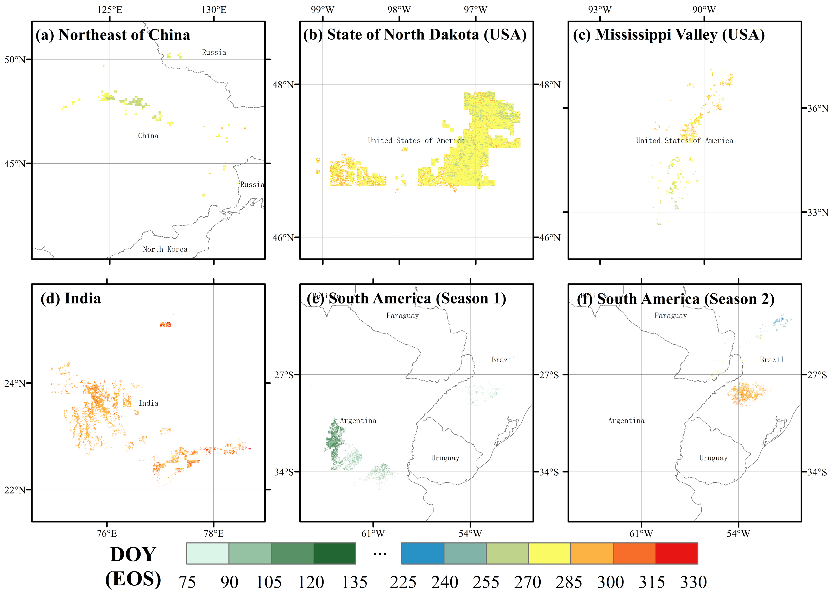
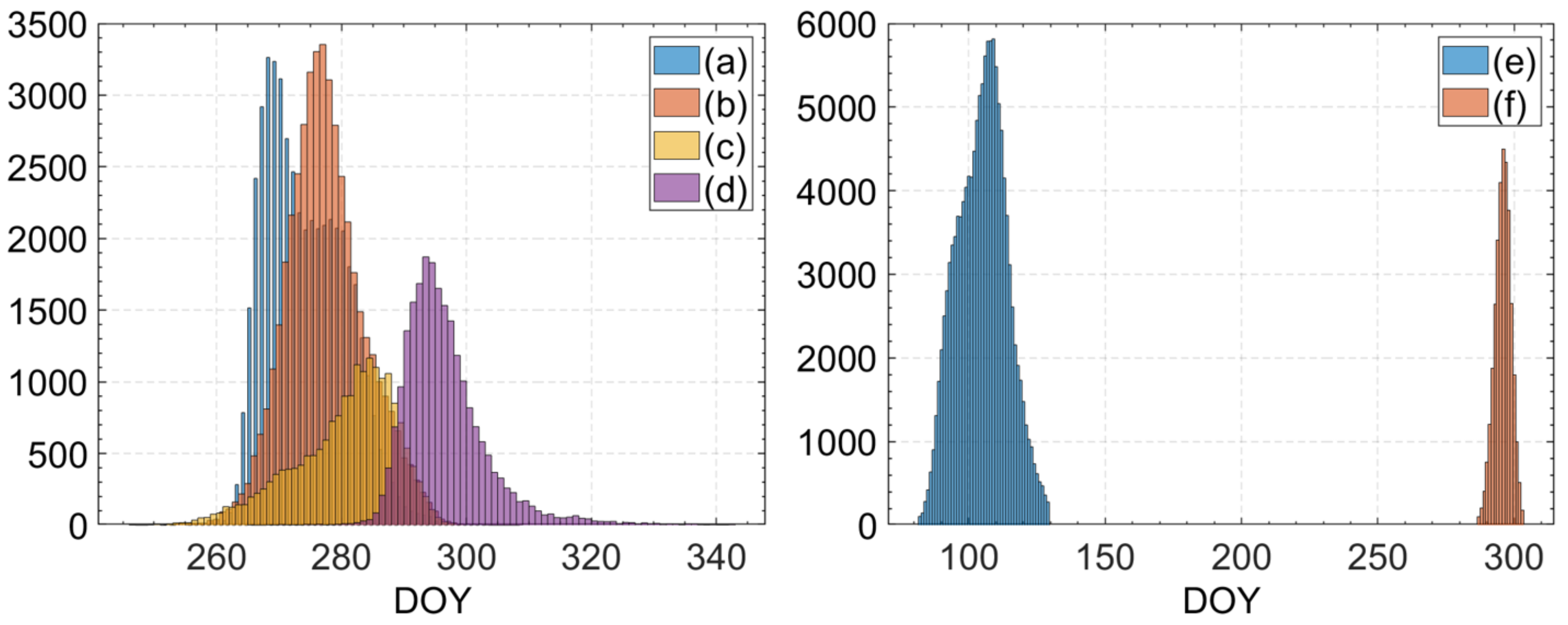
3.1. Spatial Patterns in Soybean EOS

An analysis of the multi-year EOS averages was conducted for each soybean-growing region. In the northern hemisphere, the soybean EOS dates were concentrated between DOY 262 and 310. The EOS dates for China and the United States were close to each other; the EOS in India tended to be later than in these two regions.

The main soybean-growing areas in the southern hemisphere are in South America. This region has two cropping seasons, with the first soybean crop EOS mainly between DOY 80 and 123 and the second season approximately coinciding with the northern hemisphere.

From a global perspective, by defining areas where the soybean-planting density is greater than 50% over an area of 100 km${}^2$ to be the main soybean-growing regions, these regions consist of northeast China, North Dakota, and the Mississippi River Valley in the United States, the western part of Madhya Pradesh, India, and the countries of Brazil and Argentina in South America.

It was found that the multi-year averages of the soybean EOS in northeast China are mainly concentrated between DOY 263 and 288. The spatial distributions of these dates show that the EOS gradually occurs earlier from east to west as far as the area to the northeast of Qiqihar; to the west of this, the date occurs later again (Figure 1a). Overall, the EOS in northeast China occurs slightly earlier than in North Dakota, which lies at the same latitude.

The areas where soybeans are grown are widely scattered, but the main growing regions are the Mississippi River Valley and North Dakota. These two regions are widely separated, so this paper will analyze them separately. In both regions, the multi-year average EOS was found to occur between DOY 260 and 295, with the North Dakota EOS being, on average, slightly earlier than the Mississippi River Valley EOS. In the Mississippi River Valley, the EOS occurred gradually later from south to north (Figure 1b), whereas, in North Dakota, it occurred later from east to west (Figure 1c).

In the soybean-growing region of India, the EOS onset was more concentrated within a shorter period. So, there were just a few areas of delayed EOS onset in the east of the region (Figure 1d), where the soybean EOS occurred later than in northeast China and the United States (Figure 2).

In the major soybean-growing regions of Brazil and Argentina, two cropping seasons can be extracted from the MCD12Q2 data, as shown in Figure 1e,f. For the first season, the spatial distribution patterns show that, in Argentina, the EOS of the soybean crop gradually occurred later from west to east; in the east of the region, the date of the soybean EOS is similar to that in Brazil. For the second season, the spatial distribution pattern of the EOS was mainly characterized by the early onset of the EOS in the southern growing areas and the late onset of the EOS in the northern growing areas.

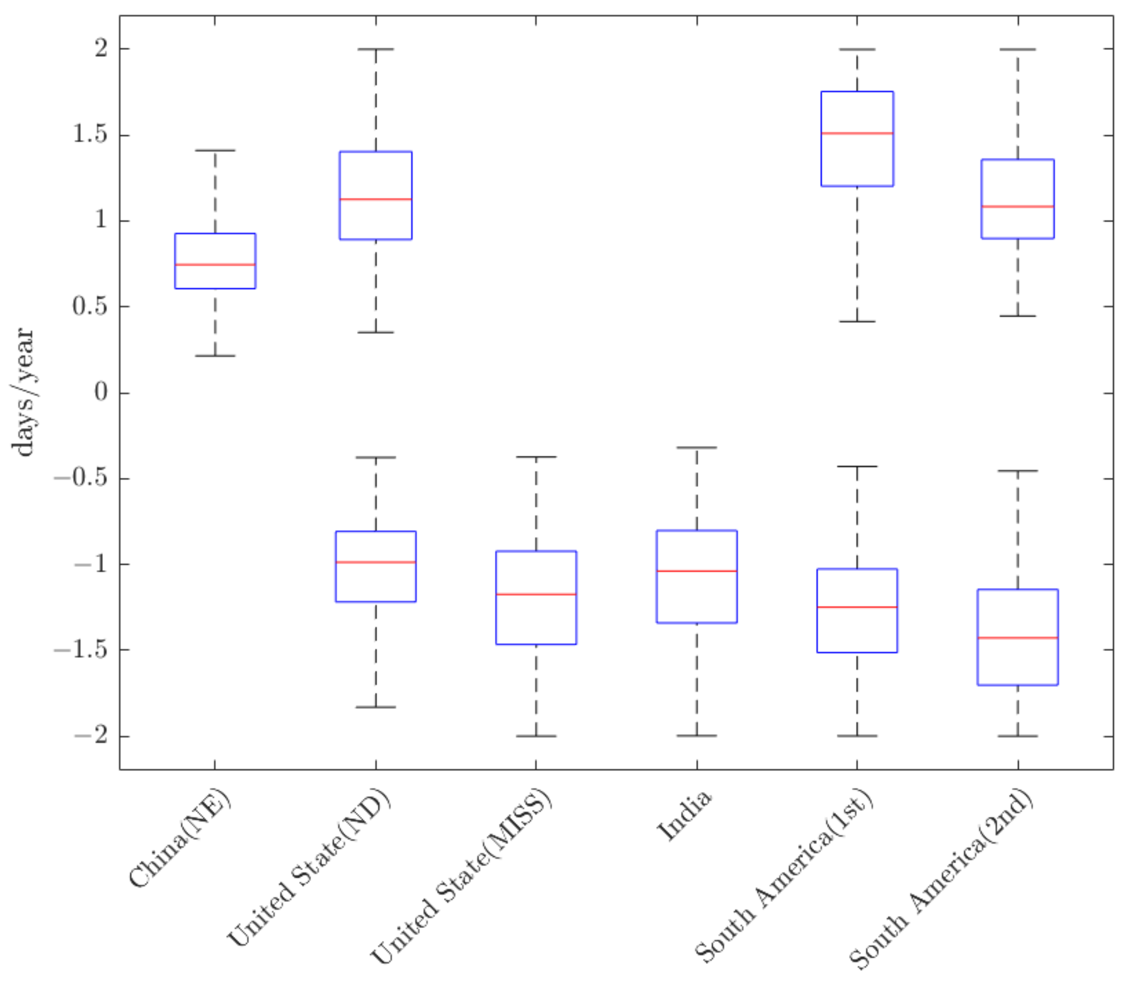
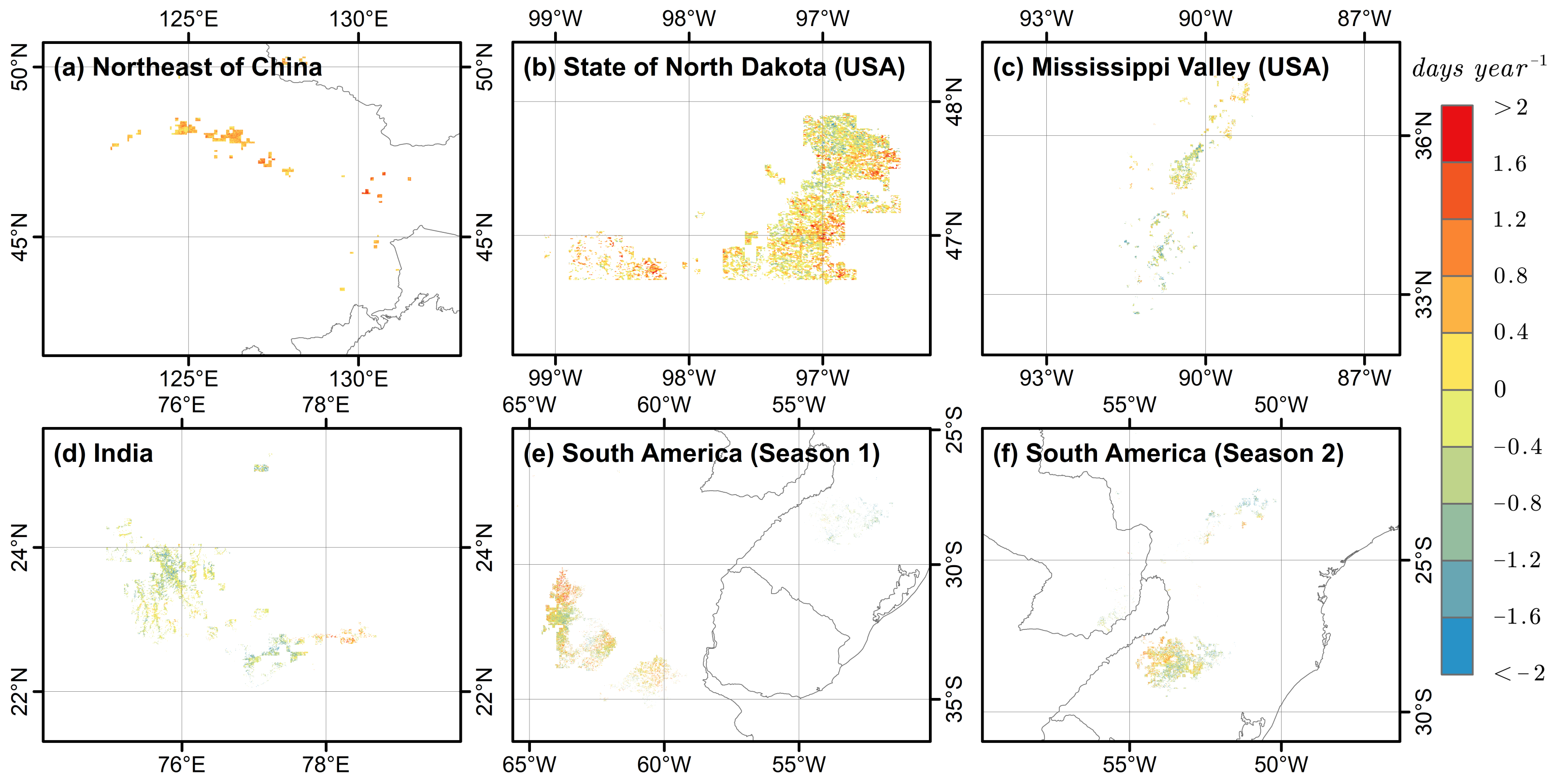
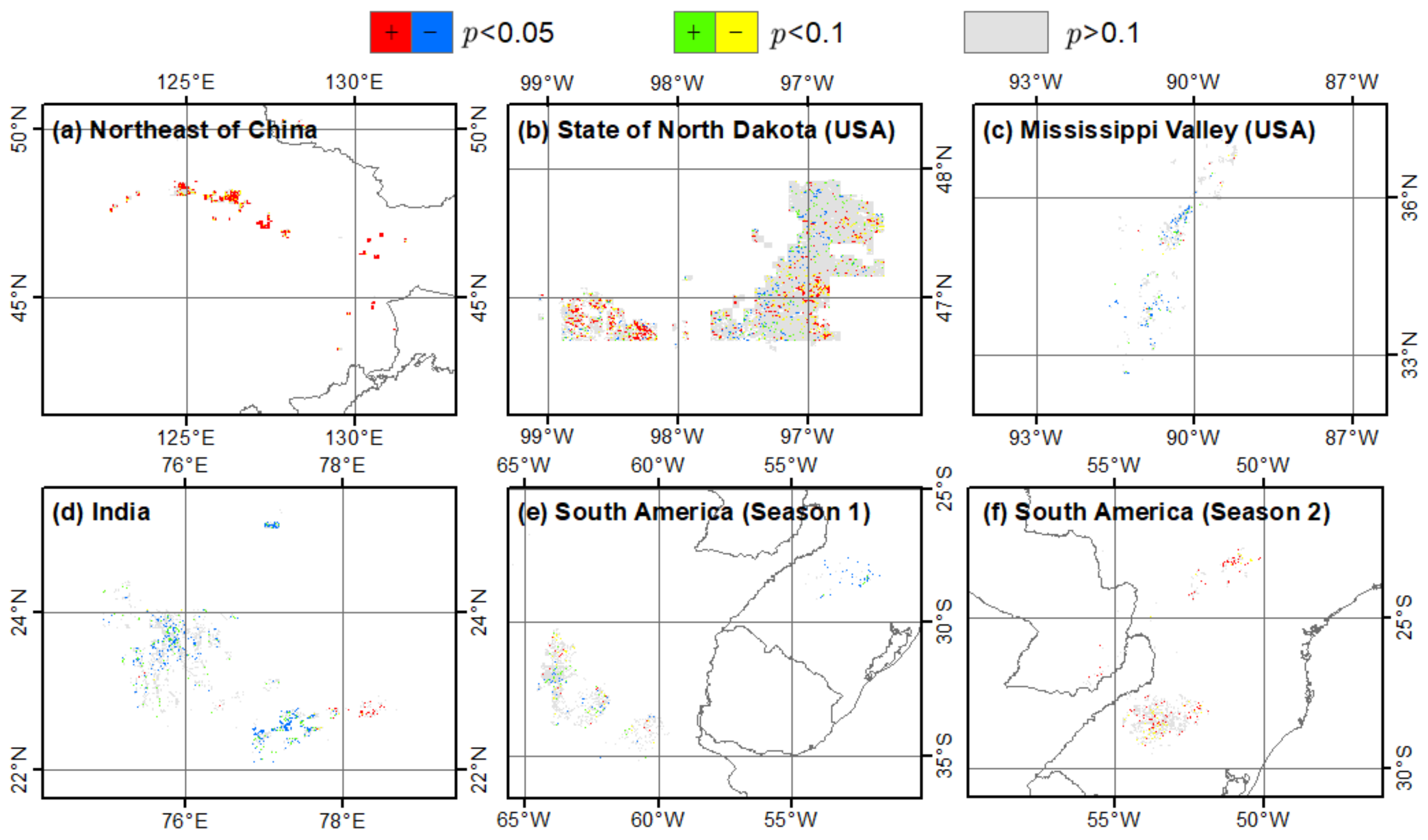
3.2. Trends and Spatial Patterns in Soybean EOS

The rate of change in the soybean EOS was ±2 days/year for most of the world’s major soybean-growing regions. The first soybean EOS tended to occur earlier in the Mississippi River Valley, India, and South America, whereas it tended to be delayed in northeast China. Many spatial variabilities were observed in the second soybean EOS in the Mississippi River Valley and the South American soybean-growing regions.

In the major soybean-growing areas of northeast China, the soybean EOS generally occurred later, in the range of $0.61$ days/year to $0.92$ days/year (Figure 3), with an average of $0.75$ days/year. It can be seen from the spatial distribution of the rate of change that there was a gradual decrease (from east to west) in the spatial variation amount in the rate of change in the soybean EOS (Figure 4a), and that in northeast China, as a whole, the soybean EOS occurred significantly later (Figure 5a).

In the U.S., there was significant spatial heterogeneity in the EOS trends in North Dakota (Figure 4b), with the rates of change in the EOS concentrated in the ranges $-1.22$ days/year and $-0.81$ days/year and $0.89$ days/year to $1.40$ days/year and $0.89$ days/year to $1.40$ days/year (Figure 3). The corresponding mean rates of change were $-0.98$ days/year and $1.13$ days/year, respectively, but the trend was insignificant in most areas (Figure 5b). At the eastern and western edges of this soybean-growing region, the EOS occurred significantly later in most places, whereas, in the center of the region, it generally occurred significantly earlier. In the major soybean-growing areas of the Mississippi River Valley, the rate of change in the EOS was found to be between $-1.47$ days/year and $-0.92$ days/year in most areas; the average rate of change was $-1.17$ days/year (Figure 3). The EOS was found to occur significantly later only in the northern part of this region (Figure 4c), where the rate of change was mainly in the range of $0.70$ days/year to $1.94$ days/year.

In the Indian soybean-growing region, the trend was mainly towards an earlier soybean EOS (Figure 4d); the rate of change was mainly in the range $-1.34$ days/year to $-0.80$ days/year, with an average of $-1.04$ days/year (Figure 3). Over most of the region, the soybean EOS occurred significantly earlier, and there was a small area in the eastern part of the growing area with a significant movement of early EOS (Figure 5d). However, there was a small area where the EOS occurred significantly later (Figure 5d).

Significant differences in the EOS trends were found for the two soybean seasons in South America. For the first season, the EOS mainly occurred earlier, with rates of change between $-1.79$ days/year and $-1.02$ days/year and an average of $-1.25$ days/year (Figure 3) in Brazil and the southern part of Colva, Argentina. The few areas where the EOS occurred significantly later were located in the northern part of Colva (Figure 4f), where the rate of change was between $1.20$ days/year and 1.75 days/year, with an average of $1.51$ days/year (Figure 3). For the second season, the rate of change in the EOS was found to be between $-2.46$ days/year to $-1.15$ days/year and from 0.90 days/year to $1.36$ days/year with average rates of $-1.43$ days/year and $1.08$ days/year, respectively, in the Londrina region and São Luiz Gonzaga (Figure 3). In the Londrina region, it was found that the soybean EOS in the eastern part of São Luiz Gonzaga occurred later. However, moving eastwards towards Passo Fundo, there was a gradual change to an earlier EOS. In the northern part of Londrina, there was a change, with EOS occurring later to earlier from south to north.

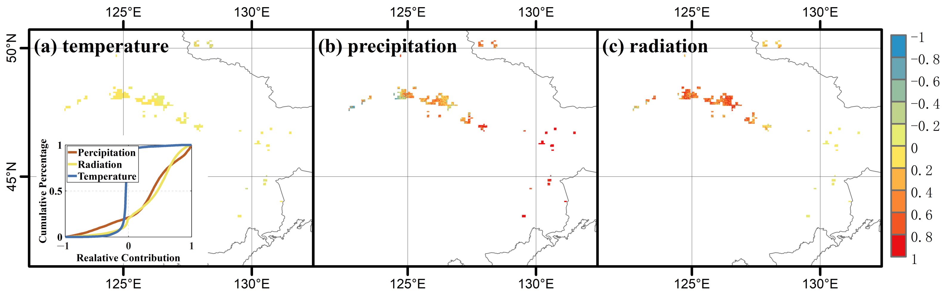
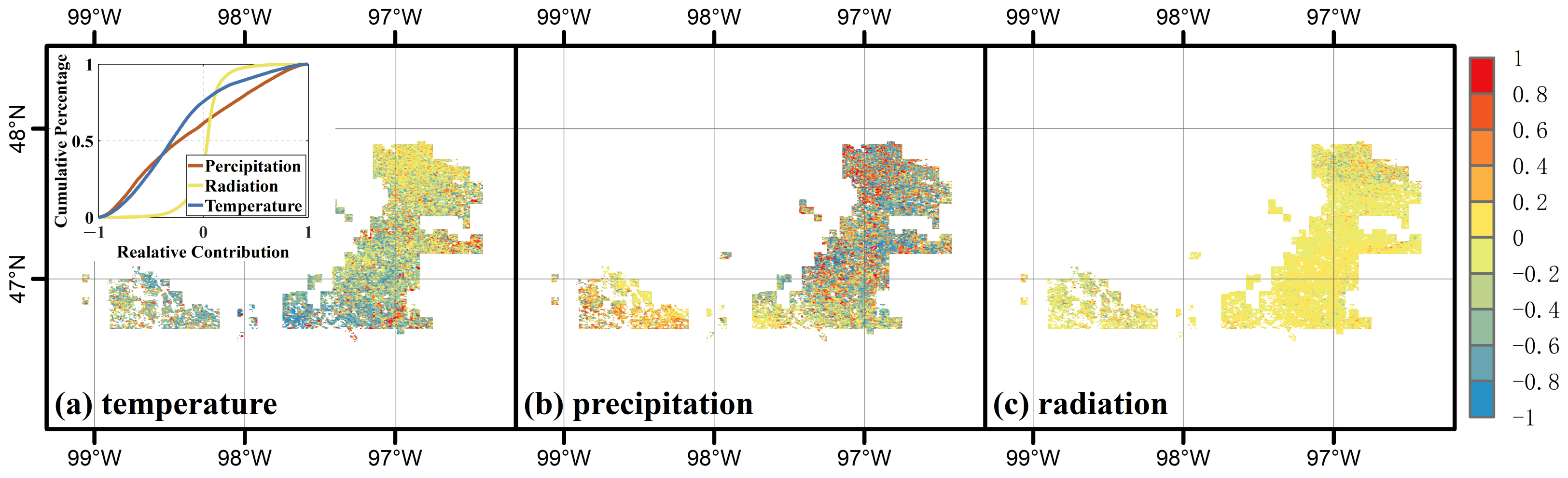
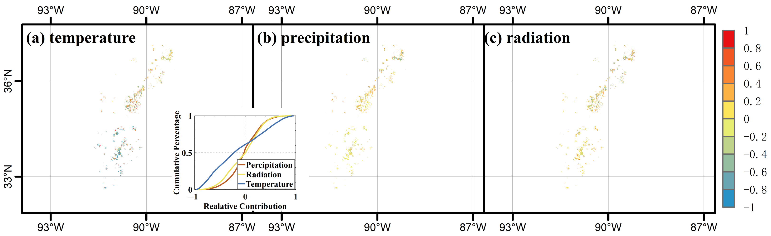
3.3. Relationship between Changes in Soybean EOS and Climate Change

The influence of different meteorological factors on the change in the soybean EOS varies from region to region. A positive contribution rate indicates that a particular meteorological factor delays the onset of the soybean EOS, whereas a negative contribution rate indicates that it contributes to an earlier onset.

Figure 6 shows the spatial distribution of the relative contributions of three meteorological factors—temperature, precipitation, and radiation—to the changes in the soybean EOS that have occurred in the major soybean-growing areas in northeast China since 2001. The main contributors to the change in the EOS in the region are precipitation and radiation, with radiation contributing an average delay of $0.92$ days/year. The spatial variation in these values is low in the east and high in the region’s west, and the contribution is positive throughout. The precipitation has contributed an average of $-19.21$% to the change in the soybean EOS in this region; the contribution is high in the east and low in the west, while some areas in the west have negative contributions. The relative contribution of the temperature to the change in the soybean EOS in this region is low (<5%).

In North Dakota and the Mississippi River Valley in the United States, the trends in soybean EOS were similarly influenced by the climate. On average, the greatest contributor to the change in the EOS is the precipitation (>40%) (Figure 7 and Figure 8). There are differences in temperature and radiation effects on the EOS in the two regions. In North Dakota, the contribution of the radiation ($-23.62$%) is smaller than that of the temperature ($-34.49$%) (Figure 7); also, the contribution of the temperature is predominantly negative. As can be seen from the cumulative frequency distribution plot, the size of the radiation contribution is relatively concentrated between $-40$% and 20%. The contribution of the temperature to the change in soybean EOS gradually changes from negative to positive from southwest to northeast. There is a lot of spatial heterogeneity in the temperature contribution in the region’s northeast, whereas the contribution size is relatively uniform in the southwest. The contribution of the radiation to the change in the EOS is relatively uniform across the region.

Similar values were found for the average relative contributions of the temperature and radiation ($-26.53$% and $-27.60$%, respectively) to the changes in the soybean EOS in the main soybean-growing areas of the Mississippi River Valley in the United States (Figure 8). There was a wide spatial variation in these contributions, with the temperature contribution changing from negative to positive from south to north. In the northern part of the region, there were some areas where all three meteorological factors made positive contributions to the change in the EOS, which means that the EOS occurred later there.

The radiation was found to be the dominant factor ($-82.75$%) affecting the soybean EOS in the main soybean-growing areas of India (Figure 9), causing the soybean EOS to occur earlier. The effects of the temperature ($8.35$%) and precipitation ($8.91$%) were relatively small. There was little spatial variation in the relative contributions of the different meteorological factors. The precipitation made a large positive contribution in some parts of the region’s west; however, even here, the negative contribution made by the radiation was still the dominant factor, trending toward an earlier EOS.

In South America, both the temperature and precipitation significantly influenced the change in the EOS for both soybean crops (Figure 10). The negative contribution due to the precipitation ($-63.82$%) in the first season was much greater than the positive contribution due to the temperature ($34.40$%); as a result, the overall trend was toward an earlier EOS. In terms of the spatial distribution, in the western part of Argentina, the contribution of precipitation was mainly negative; this changed to a positive contribution farther east. The positive contribution made by the temperature in the eastern part of the soybean-growing region of Argentina was greater than that made by the precipitation.

In the second soybean cultivation season in South America (Figure 11), the effects of the temperature ($-50.29$%) and precipitation ($49.23$%) on the soybean EOS were relatively uniform across the region. In the southern part of Brazil, the contribution of the radiation to the change in the EOS was also relatively spatially heterogeneous and made a positive contribution overall.

4. Discussion

4.1. Feasibility of Using Remote Sensing Phenology Products to Extract Soybean Crop Weather

In many previous studies, remote sensing data were used for surface vegetation or crop phenology feature extraction [27,35,36]; various vegetation phenology detection methods have been developed using the MCD12Q2 product as a source of crop phenology or vegetation data. There have been fewer studies using MCD12Q2 as a direct source of vegetation or crop parameter data [37,38].

At the pixel scale, the differences in soybean crops can be significant: sowing dates can differ by more than one month and harvest dates by more than two months over distances of 1–2 km [36]. Therefore, the direct use of MCD12Q2 for extracting soybean crop phenology is feasible but not very robust. Even though this product has the highest spatial resolution (500 m) of the surface vegetation phenology datasets that are publicly available, there is still a temporal bias, as many types of features or features entering the same phenological stage can be visible in one pixel. Due to the scale of these data, there is a problem of bias in the weather parameter estimation due to the occurrence of multiple plant species in an image or the time bias of the same species entering the same phenological stage [39]. Therefore, in this study, the soybean crop calendar published by the USDA was used as a reference to filter the EOS extraction results. After filtering, it was still found that a histogram showing the dates of occurrence of the critical phenological stages, based on MCD12Q2 data of the Indian soybean-growing areas, did not match the calendar for the Indian soybean crop and, overall, the dates seemed to be in advance of those given in the crop calendar. In the case of the main soybean-growing region of Brazil, the key weather events that influence the soybean crop have a clear bimodal distribution. Thus, two soybean crops can be grown in this region each year [36]; some studies have demonstrated the feasibility of using MCD12Q2 data to extract weather information related to the two crops [40].

It is feasible to use the MCD12Q2 data product directly as a single source of phenology information for soybean crops. However, attention should still be paid to the resolution of remote sensing phenology products as this affects the surface vegetation phenology information that they provide and to the local farming system. In this paper, SPAM 2010 statistics were used as the final source of high-density soybean planting sample units in the major soybean growing regions of the world, with the addition of CDL data as sample expansions in the U.S. region, while other regions did not have such high-precision crop samples as an aid, and soybean EOS extraction was more susceptible to other vegetation or crop influences. In future research, time-series of vegetation indices should be used to extract soybean crop phenology information so that spatial and temporal analyses can be performed after accurate information on the distribution of the soybean crop has been obtained.

4.2. Impact of Climate Change on the Spatial and Temporal Heterogeneity of Soybean EOS

This study shows that climate variability affects the date of occurrence of the soybean EOS in the world’s major soybean-growing regions. However, this effect varies by region, and even within regions experiencing similar changes in the climate, there is a large degree of spatial and temporal heterogeneity in the EOS trends. This is because the spatial resolution of the soybean EOS data extracted from the MCD12Q2 product in this study was 500 m, whereas the spatial resolution of the meteorological data used was 10 km. The values of the meteorological data raster are characterized by relatively continuous variation, as the soybean crop can have large differences in the phenological periods of adjacent fields at the pixel scale [36]. Within the same local area, the same meteorological factor can make opposing contributions to the changes in the soybean EOS. The spatial distributions of the contributions of temperature and precipitation to the trends in the soybean EOS were found to have a directional pattern in northeast China and the Mississippi River Valley in the U.S. In North Dakota, both the precipitation and temperature were found to have major influences on the soybean EOS, but the contributions of the precipitation to the changes in the soybean EOS were found to have high degrees of spatial heterogeneity.

In previous studies, the SOS was more often used for analyses related to climate-related trends [41,42] and less frequently studied using EOS as a vegetation parameter. An essential reason for this is that there is greater uncertainty associated with the indicators related to vegetation senescence or dormancy than those related to the start of the season. However, this uncertainty is considerably reduced when crops are studied.

5. Conclusions

In this study, the spatial and temporal patterns and trends in the timing of the soybean EOS and related climate drivers were analyzed for some of the world’s main soybean-growing regions over the period 2001–2018. The regions considered were northeast China (mainly Heilongjiang Province), the United States (the Mississippi River Valley and the state of North Dakota), India, Brazil, and Argentina. The EOS dates in China and the U.S. soybean-growing regions were similar; in India, the EOS occurred later than in the first two regions. The main soybean-growing areas in the southern hemisphere are in South America, where there are two growing seasons, with the end of the second season approximately coinciding with the northern hemisphere EOS. Variations in the EOS dates and the trends in the EOS were found both within and between the different soybean-growing regions, with $\pm 2$ days/year as the rate of change in the EOS. The rate of change in the soybean EOS and how the climate influenced this differed between the regions studied. An analysis of the relative contributions of different meteorological factors showed that the radiation was the major factor (contribution of $76.01$%) causing a delay in the onset of the soybean EOS in northeast China, whereas, in India, the radiation was mainly responsible ($-82.75$%) for the trend towards an earlier EOS. In the U.S. soybean-growing regions, there was more of a balance between the effects of the different factors, although the contribution of the precipitation to the change in the EOS was found to be relatively large (>40%). In contrast, precipitation was the major factor influencing the change in the soybean EOS (>98%).

References

1. Gale, F.; Valdes, C.; Ash, M. Interdependence of China, United States, and Brazil in Soybean Trade. In US Department of Agriculture’s Economic Research Service (ERS) Report; USDA: New York, NY, USA, 2019; pp. 1–48. [Google Scholar]
2. Meade, B.; Puricelli, E.; McBride, W.D.; Valdes, C.; Hoffman, L.; Foreman, L.; Dohlman, E. Corn and Soybean Production Costs and Export Competitiveness in Argentina, Brazil, and the United States; SSRN Scholarly Paper ID 2981675; Social Science Research Network: Rochester, NY, USA, 2016. [Google Scholar]
3. Gu, B.; van Grinsven, H.J.M.; Lam, S.K.; Oenema, O.; Sutton, M.A.; Mosier, A.; Chen, D. A Credit System to Solve Agricultural Nitrogen Pollution. Innovation 2021, 2, 100079. [Google Scholar] [CrossRef] [PubMed]
4. Zhang, S.; Zhang, J.; Bai, Y.; Xun, L.; Wang, J.; Zhang, D.; Yang, S.; Yuan, J. Developing a Method to Estimate Maize Area in North and Northeast of China Combining Crop Phenology Information and Time-Series MODIS EVI. IEEE Access 2019, 7, 144861–144873. [Google Scholar] [CrossRef]
5. He, L.; Asseng, S.; Zhao, G.; Wu, D.; Yang, X.; Zhuang, W.; Jin, N.; Yu, Q. Impacts of Recent Climate Warming, Cultivar Changes, and Crop Management on Winter Wheat Phenology across the Loess Plateau of China. Agric. For. Meteorol. 2015, 200, 135–143. [Google Scholar] [CrossRef]
6. Tan, Q.; Liu, Y.; Dai, L.; Pan, T. Shortened Key Growth Periods of Soybean Observed in China under Climate Change. Sci. Rep. 2021, 11, 8197. [Google Scholar] [CrossRef]
7. Tao, F.; Zhang, S.; Zhang, Z.; Rötter, R.P. Maize Growing Duration Was Prolonged across China in the Past Three Decades under the Combined Effects of Temperature, Agronomic Management, and Cultivar Shift. Glob. Chang. Biol. 2014, 20, 3686–3699. [Google Scholar] [CrossRef] [PubMed]
8. Arvor, D.; Dubreuil, V.; Ronchail, J.; Simões, M.; Funatsu, B.M. Spatial Patterns of Rainfall Regimes Related to Levels of Double Cropping Agriculture Systems in Mato Grosso (Brazil). Int. J. Climatol. 2014, 34, 2622–2633. [Google Scholar] [CrossRef]
9. Zhang, M.; Abrahao, G.; Thompson, S. Sensitivity of Soybean Planting Date to Wet Season Onset in Mato Grosso, Brazil, and Implications under Climate Change. Clim. Chang. 2021, 168, 15. [Google Scholar] [CrossRef]
10. Bandaru, V.; Yaramasu, R.; Pnvr, K.; He, J.; Fernando, S.; Sahajpal, R.; Wardlow, B.D.; Suyker, A.; Justice, C. PhenoCrop: An Integrated Satellite-Based Framework to Estimate Physiological Growth Stages of Corn and Soybeans. Int. J. Appl. Earth Obs. Geoinf. 2020, 92, 102188. [Google Scholar] [CrossRef]
11. Liu, L.; Zhang, X.; Yu, Y.; Gao, F.; Yang, Z. Real-Time Monitoring of Crop Phenology in the Midwestern United States Using VIIRS Observations. Remote Sens. 2018, 10, 1540. [Google Scholar] [CrossRef] [Green Version]
12. Manish, B.; Deshraj, P.; Walikar, L.D.; Vijaya, K.P.; Agrawal, K.K. Thermal and Radiation Environments for Assessing Crop-Weather Relationship of Soybean in Eastern Madhya Pradesh. J. Agrometeorol. 2021, 21, 141–147. [Google Scholar] [CrossRef]
13. Stocker, T.F.; Qin, D.; Plattner, G.K.; Tignor, M.; Allen, S.K.; Boschung, J.; Nauels, A.; Xia, Y.; Bex, B.; Midgley, B.M. Climate Change 2013: The Physical Science Basis. Contribution of Working Group I to the Fifth Assessment Report of the Intergovernmental Panel on Climate Change; Cambridge University Press: Cambridge, UK, 2014. [Google Scholar]
14. Cheng, H. Future Earth and Sustainable Developments. Innovation 2020, 1, 100055. [Google Scholar] [CrossRef] [PubMed]
15. Lamichhane, J.R.; Constantin, J.; Schoving, C.; Maury, P.; Debaeke, P.; Aubertot, J.N.; Dürr, C. Analysis of Soybean Germination, Emergence, and Prediction of a Possible Northward Establishment of the Crop under Climate Change. Eur. J. Agron. 2020, 113, 125972. [Google Scholar] [CrossRef]
16. Liu, Y.; Dai, L. Modelling the Impacts of Climate Change and Crop Management Measures on Soybean Phenology in China. J. Clean. Prod. 2020, 262, 121271. [Google Scholar] [CrossRef]
17. Ge, Q.; Wang, H.; Rutishauser, T.; Dai, J. Phenological Response to Climate Change in China: A Meta-Analysis. Glob. Change Biol. 2015, 21, 265–274. [Google Scholar] [CrossRef]
18. Richardson, A.D.; Keenan, T.F.; Migliavacca, M.; Ryu, Y.; Sonnentag, O.; Toomey, M. Climate Change, Phenology, and Phenological Control of Vegetation Feedbacks to the Climate System. Agric. For. Meteorol. 2013, 169, 156–173. [Google Scholar] [CrossRef]
19. He, L.; Jin, N.; Yu, Q. Impacts of Climate Change and Crop Management Practices on Soybean Phenology Changes in China. Sci. Total Environ. 2020, 707, 135638. [Google Scholar] [CrossRef]
20. Ray, D.K.; West, P.C.; Clark, M.; Gerber, J.S.; Prishchepov, A.V.; Chatterjee, S. Climate Change Has Likely Already Affected Global Food Production. PLoS ONE 2019, 14, e0217148. [Google Scholar] [CrossRef]
21. Titiek, I.; Yogi, S. The Effect of Planting Date and Harvesting Time on the Yield and Seed Quality of Rainy Season Soybean (Glycine max (L.) Merr.). J. Agric. Food Technol. 2012, 2, 73–78. [Google Scholar]
22. Meng, J.H.; Dong, T.; Zhang, M.; You, X.; Wu, B. Predicting Optimal Soybean Harvesting Dates with Satellite Data. In Precision Agriculture’13; Stafford, J.V., Ed.; Academic Publishers: Wageningen, The Netherlands, 2013; pp. 209–215. [Google Scholar] [CrossRef]
23. Wang, S.; Liu, F.; Zhou, Q.; Chen, Q.; Liu, F. Simulation and Estimation of Future Ecological Risk on the Qinghai-Tibet Plateau. Sci. Rep. 2021, 11, 17603. [Google Scholar] [CrossRef]
24. Amherdt, S.; Di Leo, N.C.; Balbarani, S.; Pereira, A.; Cornero, C.; Pacino, M.C. Exploiting Sentinel-1 Data Time-Series for Crop Classification and Harvest Date Detection. Int. J. Remote Sens. 2021, 42, 7313–7331. [Google Scholar] [CrossRef]
25. Salmon, J.M.; Friedl, M.A.; Frolking, S.; Wisser, D.; Douglas, E.M. Global Rain-Fed, Irrigated, and Paddy Croplands: A New High Resolution Map Derived from Remote Sensing, Crop Inventories and Climate Data. Int. J. Appl. Earth Obs. Geoinf. 2015, 38, 321–334. [Google Scholar] [CrossRef]
26. Erb, K.H.; Luyssaert, S.; Meyfroidt, P.; Pongratz, J.; Don, A.; Kloster, S.; Kuemmerle, T.; Fetzel, T.; Fuchs, R.; Herold, M. Land Management: Data Availability and Process Understanding for Global Change Studies. Glob. Chang. Biol. 2017, 23, 512–533. [Google Scholar] [CrossRef] [PubMed] [Green Version]
27. Ren, S.; Qin, Q.; Ren, H. Contrasting Wheat Phenological Responses to Climate Change in Global Scale. Sci. Total Environ. 2019, 665, 620–631. [Google Scholar] [CrossRef] [PubMed]
28. Wang, Y.; Yao, Z.; Zhan, Y.; Zheng, X.; Zhou, M.; Yan, G.; Wang, L.; Werner, C.; Butterbach-Bahl, K. Potential Benefits of Liming to Acid Soils on Climate Change Mitigation and Food Security. Glob. Chang. Biol. 2021, 27, 2807–2821. [Google Scholar] [CrossRef]
29. Strahler, A. MODIS Land Cover Product Algorithm Theoretical Basis Document (ATBD) Version 5.0. Available online: http://modis.gsfc.nasa.gov/data/atbd/atbd_mod12.pdf (accessed on 27 May 2021).
30. Gray, J.; Sulla-Menashe, D.; Friedl, M.A. User Guide to Collection 6 MODIS Land Cover Dynamics (MCD12Q2) Product; NASA EOSDIS Land Processes DAAC: Missoula, MT, USA, 2019; p. 8. [Google Scholar]
31. Frick, E.A.; Friedl, M.A.; Melaas, E.K.; Gray, J.M. A Comparison of Phenophase Transition Dates Calculated from MODIS EVI and NBAR-EVI. Agu. Fall Meet. Abstr. 2012, 2012, B11C-0438. [Google Scholar]
32. Peng, D.; Zhang, X.; Wu, C.; Huang, W.; Gonsamo, A.; Huete, A.R.; Didan, K.; Tan, B.; Liu, X.; Zhang, B. Intercomparison and Evaluation of Spring Phenology Products Using National Phenology Network and AmeriFlux Observations in the Contiguous United States. Agric. For. Meteorol. 2017, 242, 33–46. [Google Scholar] [CrossRef] [Green Version]
33. Wang, G.; Huang, Y.; Wei, Y.; Zhang, W.; Li, T.; Zhang, Q. Inner Mongolian Grassland Plant Phenological Changes and Their Climatic Drivers. Sci. Total Environ. 2019, 683, 1–8. [Google Scholar] [CrossRef]
34. Muñoz-Sabater, J.; Dutra, E.; Agustí-Panareda, A.; Albergel, C.; Arduini, G.; Balsamo, G.; Boussetta, S.; Choulga, M.; Harrigan, S.; Hersbach, H.; et al. ERA5-Land: A State-of-the-Art Global Reanalysis Dataset for Land Applications. Earth Syst. Sci. Data 2021, 13, 4349–4383. [Google Scholar] [CrossRef]
35. Yang, Y.; Tao, B.; Liang, L.; Huang, Y.; Matocha, C.; Lee, C.D.; Sama, M.; Masri, B.E.; Ren, W. Detecting Recent Crop Phenology Dynamics in Corn and Soybean Cropping Systems of Kentucky. Remote Sens. 2021, 13, 1615. [Google Scholar] [CrossRef]
36. Zhang, M.; Abrahao, G.; Cohn, A.; Campolo, J.; Thompson, S. A MODIS-based Scalable Remote Sensing Method to Estimate Sowing and Harvest Dates of Soybean Crops in Mato Grosso, Brazil. Heliyon 2021, 7, e07436. [Google Scholar] [CrossRef]
37. Gonsamo, A.; Chen, J.M. Circumpolar Vegetation Dynamics Product for Global Change Study. Remote Sens. Environ. 2016, 182, 13–26. [Google Scholar] [CrossRef] [Green Version]
38. Xu, L.; Niu, B.; Zhang, X.; He, Y. Dynamic Threshold of Carbon Phenology in Two Cold Temperate Grasslands in China. Remote Sens. 2021, 13, 574. [Google Scholar] [CrossRef]
39. Peng, D.; Wang, Y.; Xian, G.; Huete, A.R.; Huang, W.; Shen, M.; Wang, F.; Yu, L.; Liu, L.; Xie, Q.; et al. Investigation of Land Surface Phenology Detections in Shrublands Using Multiple Scale Satellite Data. Remote Sens. Environ. 2021, 252, 112133. [Google Scholar] [CrossRef]
40. Xiao, W.; Sun, Z.; Wang, Q.; Yang, Y. Evaluating MODIS Phenology Product for Rotating Croplands through Ground Observations. J. Appl. Remote Sens. 2013, 7, 073562. [Google Scholar] [CrossRef]
41. Sacks, W.J.; Deryng, D.; Foley, J.A.; Ramankutty, N. Crop Planting Dates: An Analysis of Global Patterns. Glob. Ecol. Biogeogr. 2010, 19, 607–620. [Google Scholar] [CrossRef]
42. Begue, A.; Vintrou, E.; Saad, A.; Hiernaux, P. Differences between Cropland and Rangeland MODIS Phenology (Start-of-Season) in Mali. Int. J. Appl. Earth Obs. Geoinf. 2014, 31, 167–170. [Google Scholar] [CrossRef]
Figure 1. Spatial patterns in EOS multi-year averages for soybeans in different soybean-growing regions: (a) northeast China; (b) North Dakota, U.S.; (c) Mississippi River Valley, U.S.; (d) India; (e) South America (first crop); and (f) South America (second crop).
Remotesensing 14 01867 g001
Figure 2. Histogram showing the temporal distributions of the EOS in each major soybean-producing region (left: northern hemisphere, right: southern hemisphere): (a) northeast China; (b) North Dakota, U.S.; (c) Mississippi River Valley, U.S.; (d) India; (e) South America (first crop); and (f) South America (second crop).
Remotesensing 14 01867 g002
Figure 3. Ranges concerning the rates of change in the soybean EOS for the major soybean-producing regions of the world.
Remotesensing 14 01867 g003
Figure 4. Analysis of trends in soybean EOS for the major soybean-growing regions.
Remotesensing 14 01867 g004
Figure 5. Spatial distribution of the rate of change in the soybean EOS for the major soybean-growing regions: red and blue indicate areas where the soybean EOS occurs significantly earlier and significantly later, respectively; green and yellow indicate areas where the soybean EOS occurs slightly later and slightly earlier, respectively; and grey indicates that there is no significant trend in the soybean EOS.
Remotesensing 14 01867 g005
Figure 6. Relative contribution of different meteorological factors to the change in the soybean EOS in the major soybean-growing areas in northeast China.
Remotesensing 14 01867 g006
Figure 7. Relative contributions of different meteorological factors to the change in the soybean EOS in the major soybean-growing areas in North Dakota, U.S.
Remotesensing 14 01867 g007
Figure 8. Relative contributions of different meteorological factors to the change in the soybean EOS in the major soybean-growing areas in the Mississippi River Valley, U.S.
Remotesensing 14 01867 g008
Figure 9. Relative contributions of different meteorological factors to the change in the soybean EOS in the major soybean-growing areas in India.
Remotesensing 14 01867 g009
Figure 10. Relative contributions of different meteorological factors to the change in the soybean EOS in the major soybean-growing areas in South America (first season).
Remotesensing 14 01867 g010
Figure 11. Relative contributions of different meteorological factors to the change in the soybean EOS in the major soybean-growing areas in South America (second season).
Remotesensing 14 01867 g011
Publisher’s Note: MDPI stays neutral with regard to jurisdictional claims in published maps and institutional affiliations.