Article

Effects of Increasing C4-Crop Cover and Stomatal Conductance on Evapotranspiration: Simulations for a Lake Erie Watershed

by
Chathuranga Kumara Senevirathne
*,
Anita Simic Milas
,
Ganming Liu
,
Margaret Mary Yacobucci
and
Yahampath Anuruddha Marambe
Department of Geology, School of Earth, Environment and Society, Bowling Green State University, Bowling Green, OH 43403, USA
*
Author to whom correspondence should be addressed.
Remote Sens. 2022, 14(8), 1914; https://doi.org/10.3390/rs14081914
Submission received: 2 March 2022 / Revised: 12 April 2022 / Accepted: 13 April 2022 / Published: 15 April 2022

Abstract

:
Accurate quantification of evapotranspiration (ET) is crucial for surface water resources and best agricultural management practices in watersheds. The aim of this study was to better understand ET changes caused by the rapid expansion of C4 (corn) cover and rapid changes in stomatal conductance, which may be amplified in the future due to environmental and human-contributing factors, such as climate change and agricultural practices. Linking the enlargement of agricultural land with the physiological properties of crops, such as photosynthetic adaptations and stomatal conductance, is necessary to explore the magnitude of these impacts. This study examined the effects of increased C4 (corn) crop cover and stomatal conductance on evapotranspiration (ET) rates in the Lower Maumee River Watershed, Ohio, USA, during the 2018 growing season. Simulation results using a modified-for-crops version of the Boreal Ecosystem Productivity Simulator (BEPS) showed that a hypothetical increase of corn cover by as much as 100% would not significantly impact the watershed ET rate, with a 5.05% overall increase in ET in July and a 3.96% increase in August. Changes in the stomatal conductance of crops, however, impacted ET more. The results showed a significant increase in the ET rate (up to 24.04% for corn and 5.10% for soybean) for the modeling scenario that integrated high stomatal conductance, which agreed with the thermal-based ECOSTRESS ET product derived over the study area (+/−0.9 mm day−1) for the same period. We suggest that the alteration of the crop stomata mechanism, caused largely by rapid climate change and intensive farming practices, should be carefully quantified, and its impact on hydrology at the ecosystem level further explored.

Graphical Abstract

1. Introduction

Evapotranspiration (ET) is the second largest component of the terrestrial hydrological cycle. It was estimated that approximately 60% of annual global land precipitation returns to the atmosphere through ET [1,2], while the values could reach 70% on average in the USA and could be even higher than 90% in the Western and Midwestern USA [3]. As the link between energy, water, and carbon cycles, ET is sensitive to a range of natural and human-induced factors, making its prediction a challenging task. Among the critical factors are meteorological variables, soil properties, and vegetation parameters measured on different scales, from leaf to ecosystem levels [4].
Rapid expansion of agricultural land and accelerated development of productivity-enhancing technology and chemical applications impact the microclimate and local hydrology of a watershed through various mechanisms. For example, spatiotemporal changes in the vegetation cover control changes in canopy structural parameters, such as leaf area index (LAI) and leaf clumping, which are instrumental in the mass, energy, and momentum exchange between canopy and the atmosphere. LAI drives canopy radiation extinction, water interception, and water vapor and carbon gas exchanges [4,5,6,7], while the clumping index affects the amount of sunlit and shaded leaf areas, alters LAI, and ultimately impacts the ET rate [4,8,9,10].
One of the most critical leaf- and canopy-level parameters in quantifying hydrological processes is stomatal resistance, or its inverse stomatal conductance [11,12]. Stomatal resistance is related to the bulk surface resistance caused by the crop type and its photosynthetic mechanism, crop growth stage, roughness length, and wind speed [11,13]. Stomatal resistance/conductance is sensitive to factors such as soil moisture, atmospheric pCO2, and weather parameters such as air temperature, relative humidity, and solar radiation [12,14]. As such, stomatal resistance/conductance regulated the rate of transpiration, CO2 intake from the atmosphere, and water uptake from soil [15]. In addition to these natural mechanisms, two anthropogenic factors, climate change and agricultural practices, may considerably alter plants’ uptake of water from soil and CO2 intake from the atmosphere and soil, and ultimately affect stomatal conductance and the ET rate. For instance, rising air temperature increases stomatal conductance despite a decrease in leaf water potential or an increase in intercellular CO2 concentration [14]. On the other hand, stomatal conductance decreases in response to the depletion of soil moisture content [12], which increases with more frequent occurrences of drought-heat waves.
With respect to agricultural practices, several studies have confirmed that monoculture farming and agricultural practices could lead to a substantial change in ET [3,13,16,17] by controlling crop density and root water absorption capacity [13,18,19]. Zou et al. [20] reported that agricultural chemicals and irrigation increased ET per unit area at rates of 60.93%, while climate change, including precipitation and relative humidity, contributed to an increase of 28.01% for the same area. One of the major crops that is grown as monoculture is corn (maize), which has become a critical crop not just in the Midwest but across the USA and worldwide due to its high productivity and versatility [21,22,23]. Corn is cultivated as grains for animal and human feeding, and it represents 40% of the global grain product [24]. Daily biofuel production in 2017 was nearly 1000 barrels per day, which further increased the need for corn production in the USA [25]. In addition to the rapid expansion of corn-covered land, the corn’s C4 photosynthetic system differs from the C3 photosynthetic system of other key crops, such as soybean and wheat, resulting in a different behavior of the stomatal conductance apparatus and ultimately the ET rate. Therefore, the reduction of C3 and the expansion of C4 crop cover must be considered to accurately estimate the ET rate in a watershed.
C4 plants are more photosynthetically active than C3 plants due to their anatomic adaptations [26,27]. The anatomical variation of C4 plants results in more efficient CO2 fixation and decreased photorespiration, the waste product of photosynthesis [28,29]. These properties are related to high water use efficiency (WUE), a function of primary production and transpiration, which helps C4 plants to survive better in drier environments [30,31]. High leaf vein density and their leaf distribution pattern are other factors that influence WUE and photosynthetic efficiency in C4 plants [32].
Linking the enlargement of agricultural land with the physiological properties of crops, such as their photosynthetic adaptations and stomatal conductance, is possible using remote sensing-based models. Remote sensing technology is used to capture Land Use/Land Cover (LULC) changes and land heterogeneity over large areas, which is instrumental for the accuracy of spatial ET estimations. ET models are mainly based on either thermal information or stomatal conductance process approaches [33,34,35]. While surface energy balance models (SEBs), which are temperature-based, are more effective for water-stressed soil conditions and surfaces where sensible heat flux is extensive, stomatal conductance-based models are optimal for places such as heterogeneous vegetated surfaces where sensible heat flux is low [7,10]. The main difference between the two methods is that the conductance-based models use vegetation structural information and optical remote sensing images to quantify canopy conductance and ET [10,36], while the temperature-based models use land surface temperature to estimate sensible heat flux and derive ET as a residual of the surface energy balance. In this study, a version of the Boreal Ecosystem Productivity Simulator (BEPS), a stomatal conductance-process model developed at the Canada Center for Remote Sensing [33], that was modified for crops was used to estimate ET rates in the Lower Maumee River Watershed in Ohio. The resulting watershed ET rates were then compared to the ECOSTRESS thermal-driven ET product generated and validated against the FLUXNET measurements by the NASA Land Processes Distributed Active Archive Center (LPDAAC) [37].
The Lower Maumee River watershed is under a high amount of stress due to chemical loading into the river from surrounding agricultural land, urbanization, and stream channelization [38,39]. High sedimentation and nutrient pollution impact the water quality of the river, and constant LULC changes affect the overall water budget of the watershed [39]. The increased surface runoff and peak runoff led to increased flooding and decreased groundwater recharge. Additionally, the loss of natural vegetation alters ET [38]; thus, maintaining the optimal ET rate is critical to keeping the water cycle components in balance and preserving the well-being of a watershed.
In this study, two hypothetical impact scenarios for ET simulations using the modified BEPS model were designed to explore: (1) how incremental increases of corn cover, as a C4 crop replacing C3 crops such as soybean, winter wheat/cover crop, and alfalfa at the rate of 10% per cover increment, would impact the watershed ET rate, and (2) how alterations of stomatal conductance of key crops would impact the watershed ET rate. Daily and monthly time series of ET were generated over the Lower Maumee River watershed in the 2018 growing season. The overall goal of this proof-of-concept study was to better understand ET changes due to the rapid expansion of C4 (corn) cover and rapid changes in stomatal conductance, which are becoming increasingly altered by human-contributing factors, such as climate change and agricultural practices. To the best of our knowledge, no study has investigated the effects of increasing C4-crop cover and stomatal conductance on crop ET.

2. Materials and Methods

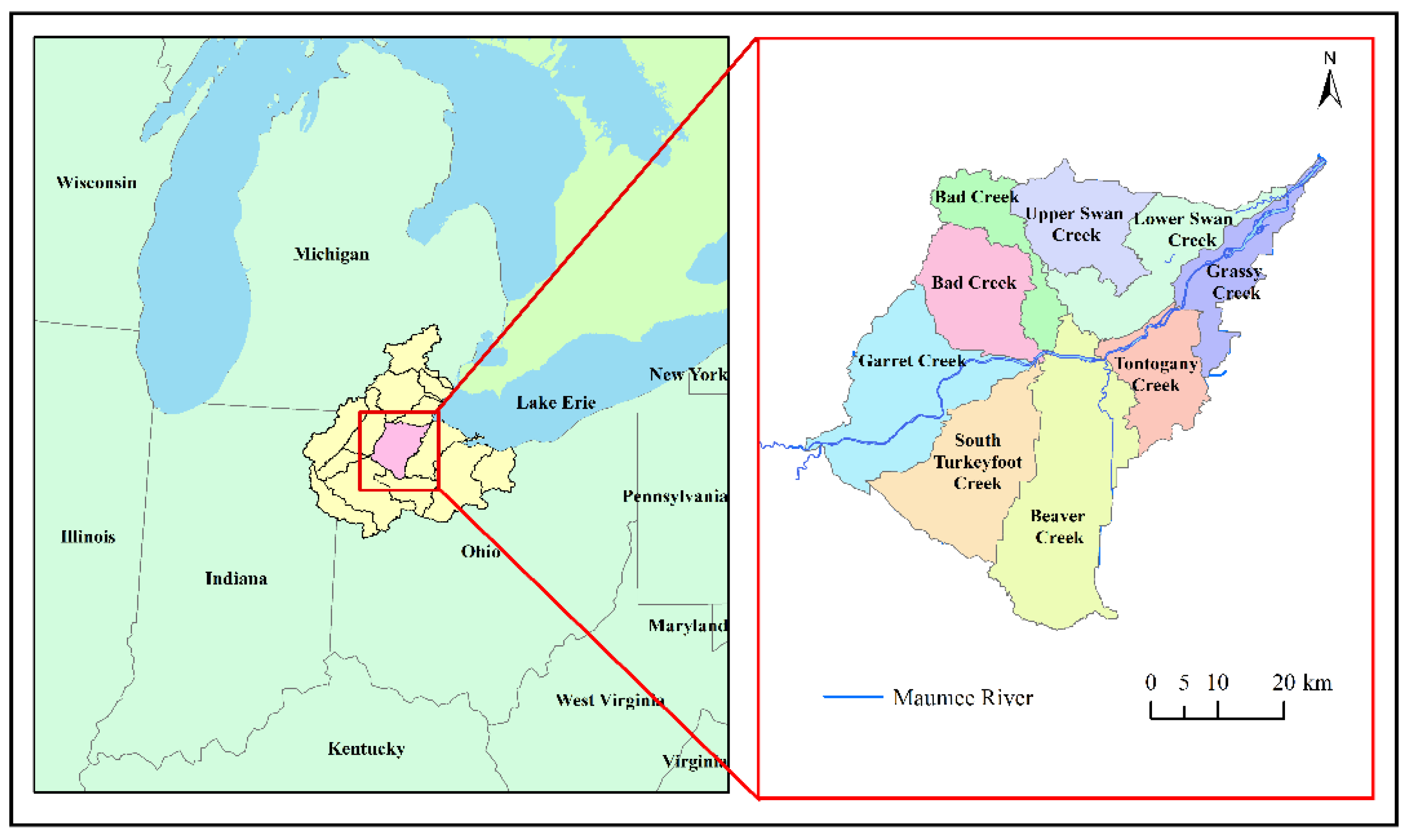
2.1. Description of Study Area

The Lower Maumee River watershed (Hydrologic Unit Code [HUC] 04100009) was selected as the study site. The watershed covers parts of Lucas, Fulton, Henry, Wood, Defiance, Putnam, and Hancock Counties in the state of Ohio, USA (centered at latitude 41.410 N and longitude 83.940 W) (Figure 1). The Lower Maumee River drains into the Western Lake Erie Basin. More than 88.1% of the watershed is relatively flat, with a slope of 2% or less, and the average elevation of the study area is 200 m [40]. The study area has a humid continental climate (Köppen-Geiger classification Dfa; Beck et al., 2018), with a mean annual temperature of 10 °C and mean annual precipitation of 948 mm/year [41]. Winters are cold (average temperature −2.4 °C) and summers are hot (average temperature 22.1 °C). Precipitation is somewhat higher in summer (91.7 mm month−1) and spring (87.0 mm month−1) than in autumn (75.4 mm month−1) and winter (61.9 mm month−1). Due to anthropogenic warming, the region is projected to shift to a humid subtropical climate (Köppen-Geiger classification Cfa) within the next 50–80 years [42].
Limestone, shale, and dolostone of Paleozoic age are the main bedrock types found in the area. Among the 317 different soil types that have been identified within the Lower Maumee River watershed, glacial till, glacial outwash, lacustrine beach deposits, recent alluvium, and weathered bedrock materials mixed with organic materials are the dominant soil types. Soil in the area has poor draining properties due to its flat topography (40). In 2018, approximately 84.2% of the watershed area was covered by croplands, and according to the United States Agriculture Department (USDA) [43] classification, about 37.9% of the watershed area was covered with soybean, 26.4% with corn, 7.4% with deciduous forest, and 5.8% of the watershed was covered with winter wheat, which is commonly replaced with cover crops in the summer season.
Figure 1. Location of study area—The Lower Maumee River watershed in Ohio, USA. The watershed drains into Lake Erie (Data Source: USGS [44]).
Remotesensing 14 01914 g001

2.2. Data

2.2.1. Meteorological Data

A series of grid meteorological (gridMET) data, developed by the Climatology Lab, was used in this study ([45]). Allen et al. [46] used the gridMET data set to develop the Earth Engine Evapotranspiration Flux (EEFlux) application, and they successfully calculated ET using a surface energy balance method. The gridMET data were derived using two types of data sets, namely the North American Land Data Assimilation System Phase 2 (NLDAS-2) and Parameter-elevation Regressions on Independent Slopes Model (PRISM). The NLDAS-2 data set is derived from the North American Regional Reanalysis (NARR) data, and the final data product has a spatial resolution of 12 km and temporal resolution of one hour. The non-commercial PRISM data have an 800-m spatial resolution and one-month temporal resolution [47]. By merging both the NLDAS-2 and PRISM data sets, the final meteorological data are set to a spatial resolution of 4 km and a temporal resolution of one day; the data can be downloaded in the netCDF file format. The downloaded meteorological data were further processed with ArcMap, which involved resampling the data to 30-m spatial resolution using the nearest-neighbor resampling methods and converting them to the binary file format that is used by BEPS [4].” The programing language Python within ArcGIS was used to automatize the resampling and georeferencing processes of the large number of meteorological images. For a single day, there were six types of binary meteorological input files, and altogether about 180 files for each month were prepared and used in the model. The meteorological data included total incoming radiation, maximum and minimum temperature, mean of maximum and minimum relative humidity, and total precipitation. The outputs of the model were daily ET images (mm day−1), which were averaged to derive monthly information.

2.2.2. Satellite Imagery Data and Products

Six nearly cloud-free Landsat 8 Operational Land Imager (OLI) surface reflectance data (Collection 2/Level 2) were used to derive vegetation indices and LAI maps [44]. Sentinel-2A/2B MSI images were used as supplemental information to replace about 15% of the cloudy pixels from the two Landsat images [48] (Table 1).
Before fusing the information from the satellite data sets, Sentinel-2A/2B images were spatially aggregated to 30-m spatial resolution. The regression models, defined between Sentinel-2 and Landsat 8 data for each band based on clear (cloudless) pixels, were applied to Landsat 8 pixels that contained clouds or cloud shadows. This pixel-by-pixel approach was found to be a reliable gap-filling method [49]. Mandanici and Bitelli [50] identified a strong correlation between the corresponding spectral bands of Sentinel-2 and Landsat 8 imagery. Useya and Chen [51] also successfully combined pixels from cloud-free Sentinel-2 and Landsat 7 data to fill the gaps in Landsat 8 images. The ENVI 5.5.2 software package was used to fill the gap.

2.2.3. Land Use/Land Cover (LULC) Data

The land cover product generated by the United States Department of Agriculture (USDA) National Agricultural Statistics Service (NASS) was downloaded using the Cropland Data Layer (CDL) [52]. According to the USDA [52], the classification accuracy of the land cover data was 90% for corn, soybean, and wheat, and 80% for other crops. The data product was available at 30-m spatial resolution, which matched other Landsat 8-based products used in the BEPS simulations.
The dominant land cover types in the study area were corn, soybean, deciduous forest, winter wheat/cover crops, grass, and alfalfa (Figure 2). There were also small areas covered with some other vegetation that were reclassified and assigned to the most similar key crops to satisfy the input requirements of BEPS. For instance, sorghum was reclassified as corn because of its C4 photosynthetic pathway.

2.2.4. Leaf Area Index

The selected algorithms were based on vegetation indices from the literature that were coarsely validated over a nearby research area throughout the 2017 growing season to account for crop phenology and soil exposure [53] (Table 2). The soil-adjusted vegetation index (SAVI) [54] was used to suppress the effects of soil pixels at the beginning of the growing season. Hong et al. [55] developed an empirical equation between LAI and SAVI, and this relationship was applied to corn and soybean during the early and later stages of the growing seasons (May and September) in this study (Table 3). The empirical relationship between the Enhanced Vegetation Index (EVI) and ground-measured LAI derived by Kang et al. [56] was used to estimate the LAI of corn, soybean, and grass during June, July, and September (Table 3). In addition, empirical relationships between LAI and EVI, developed by Boegh et al. [57], were used for winter wheat/cover crops, alfalfa, and deciduous crops (Table 3). Similarly, the Simple Ratio (SR)-based empirical formula suggested by Blinn et al. [58] was used for the LAI estimation of conifers (Table 3).
Given that LAI of crops changes rapidly and that access to cloud-free satellite data was limited, the statistical interpolation technique based on the linear regression between the existing images was used to create a required series of LAI images every 8–10 days [4,13]. This was a pixel-by-pixel operation, and a Python code was developed to automate the process.

2.2.5. ECOSTRESS Data

To validate the ET outputs of the BEPS simulations, the ECOSTRESS-generated ET product was used. ECOSTRESS collects data at 38 m × 69 m resolution at nadir with a rapid revisit time of 1–5 days, which are then resampled to 70 m × 70 m to minimize noises and stored in the Hierarchical Data Format version 5 (HDF5). ECOSTRESS ET data are regularly validated against the Fluxnet ET field data [59,60] before they are published; therefore, the ECOSTRESS ET product was used as the reference point for validation of the BEPS estimates derived in this study.
The ECOSTRESS ET product was generated by NASA Land Processes Distributed Active Archive Center (LPDAAC) using the Dis-ALEXI model, and the product was validated against the Fluxnet field measurements [37]. The ECOSTRESS ET product was downloaded from the NASA Earthdata—“ECOSTRESS” web portal, and the ECOSTRESS_swath2grid.py script, available on the NASA website, was used to convert ECOSTRESS swath data products into projected GeoTIFFs. The GeoTIFF images were resampled to 30 × 30 m to match the spatial resolution of other BEPS input data. As the ECOSTRESS images did not fully cover the study area, validation over the whole site was slightly limited (Figure 3).

2.2.6. Available Water Holding Capacity (AWHC) Data

Along with LAI and leaf clumping index measurements, soil water holding capacity is critical in calculating canopy conductance [33]. Available water holding capacity (AWHC) data used in the modeling were extracted from the USDA Natural Resources Conservation Service, which provides soil maps and related data for more than 95 percent of the nation’s counties [61]. Using the USDA’s ArcGIS toolbox called SSURGO downloader, data were downloaded for the soil depth of 150 cm [62].

2.3. Evapotranspiration Modeling

2.3.1. BEPS Model

BEPS effectively reflects the physical concept of an ecosystem by utilizing weather parameters, plant structural parameters, and photosynthetic processes and their impact on the ET rate [4,5,33,63]. BEPS is a process-based model that utilizes the two-leaf model, and it considers the stratification of sunlit and shaded leaves separately for photosynthesis and transpiration modeling [4,10]. The BEPS model is more effective in generating canopy photosynthesis than the big-leaf model, as it can better capture the nonlinear response of fluxes such as water, heat, and CO2. The photosynthetic model is combined with the stomata model based on stomatal conductance. A modified Ball-Berry model, which considers the influence of soil water, is used to describe stomatal conductance [64]. The extended Norman’s method [65] is used in BEPS to calculate the LAI for sunlit and shaded leaves while considering the effect of foliage clumping [64]. BEPS can run on a daily and hourly scale. LAI and meteorological data are time-dependent inputs to the BEPS model. LAI is calculated using remote sensing-derived vegetation indices using corresponding empirical algorithms [56]. In this study, BEPS was modified for C4 (corn) and C3 crops (soybean, winter wheat/cover crops, and alfalfa). Several parameters, such as clumping index and stomatal resistance/conductance were adjusted accordingly, and various empirical algorithms were utilized to estimate LAI accurately [53]. More details about BEPS can be found in [5,33].

2.3.2. Hypothetical Impact Analyses—Alterations in Stomatal Conductance and Corn Cover Extent

Two hypothetical scenarios were considered in this study to simulate the daily and monthly ET rates of the Lower Maumee River watershed. The first analysis was a sensitivity analysis in which BEPS was run for a range of stomatal conductance values found in the literature, as shown in Table 4. Three stomatal conductance values (low, medium, and high) were selected for each cover type. The analysis first included the stomatal conductance alterations for all cover types, and then the alterations were done just for corn while stomatal conductance values of other cover types were kept constant, at medium range. The stomatal conductance values for corn ranged from 0.0040 to 0.009 ms−1 [66] (Table 4).
The second analysis considered the impact of hypothetical incremental increases in corn cover from the existing state to 100% of vegetation cover. Ten synthetic LULC images were generated, and in each image, 10% of randomly selected other-than-corn vegetation pixels were replaced with corn at each iteration. LAI images were modified for each LULC combination in such a way that the mean corn LAI values were assigned to the modified pixels, while the values stayed unchanged for the original pixels. ArcGIS was used to generate the synthetic LAI images. This process was repeatedly applied to all LAI images for the months of June, July, August, and September, and ET simulations were then conducted for each scenario (Figure 4).

3. Results

3.1. Estimated LAI

Visual observations of the derived LAI images and their monthly average values for each land cover class showed the expected increase and then decrease in the LAI trend over the growing season (Table 5, Figure 5 and Figure 6). Although the peak LAI values for most of the crops were estimated in July or August, trends differed among the crop types due to their different growing cycles (Figure 6). For instance, alfalfa is a perennial plant that is harvested several times throughout a growing season and in winter, whereas wheat is commonly harvested and replaced with cover crops early in the growing season. The mean LAI values ranged from 1.36 to 1.94 for grass, from 1.21 to 2.24 for alfalfa, and from 1.54 to 2.36 for winter wheat/cover crops during the peak of the growing season. In the case of corn and soybean, their peaks were pronounced in the middle of the summer. Corn reached its LAI maximum in mid-July (LAI = 5.10), while soybean reached its LAI maximum in August (LAI = 4.30) (Figure 5 and Figure 6). This shift in the peaks could occur due to the planting calendar, differences in physiology and photosynthesis systems of soybean and corn (C3 vs. C4), and/or soybean’s capability to fix nitrogen from soil and atmosphere. At the optimal soil temperature (15–18 °C), corn commonly emerges within 8 to 10 days, and by the peak of the growing season, corn has 8–12 leaves [73]. This stage is normally known as the vegetative stage V8, when long and wide leaf blades can be observed [74]. The estimated LAI data were generally in agreement with the LAI values from the literature (Table 6).

3.2. Estimated ET Rates under Different Stomatal Conductance Values

All three BEPS scenarios with three different stomatal conductance values showed a similar ET trend over a growing season (Figure 7). The estimated monthly ET rate increased from May to July, peaked in July or August, and decreased from August to September. It was found that the ET rate would generally increase with an increase in stomatal conductance, although not in all cases.
When considering scenario 2 (Table 7), where both main crop types (corn and soybean) were assigned the same stomatal conductance (middle value), corn had a lower estimated ET rate in August and September than soybean. In contrast, during May, June, and July, corn showed a higher ET rate than soybean (Figure 8). When stomatal conductance is increased from scenario 2 (middle value) to scenario 1 (high value), the ET rate of corn increases by 24.4% in July and 16.8% in August, and the ET rate of soybean increases by 4.7% in July and 5.2% in August. When the stomatal conductance of corn was reduced from scenario 2 (middle value) to scenario 3 (low value), the ET rate of corn decreased by 28.8% in July and 29.2% in August, while the ET rate of soybean decreased by 40.7% in July and 38.1% in August. Finally, in the case when only corn’s stomatal conductance was altered, the trend for the whole watershed showed that during the peak months (July and August), the differences between the monthly mean ET rates decreased with the decrease of stomatal conductance (Figure 9). This result agrees with the previous observations that the ET rate of corn becomes lower due to its low stomatal conductance, while the ET rate of soybean naturally increases in August (Figure 7).

3.3. Estimated ET Rates under Different Percentages of Corn Cover

Other vegetation was replaced with corn in the simulation to explore the potential effect of a shift to C4 monocrop cultivation on the ET rate of the watershed. When the corn cover increased from the existing state in 2018 to 100% of vegetated cover (Figure 10), there was a gradual increase in the ET rate for both July and August, but no significant difference in the ET rate was observed (Figure 11 and Figure 12). The change in ET showed an increase of 5.05% in July and 3.96% in August. Note, however, that the ET rate was less variable with increased corn cover.

3.4. Comparison of Daily BEPS-Generated ET and ECOSTRESS ET Product

There is general agreement between the daily ET rates generated using BEPS and ECOSTRESS (Table 7, Figure 13). The validation is based on August data, as images for other months were not available for most of the watershed (Figure 3). The best agreement was observed under the high stomatal conductance scenario for corn and under the high/medium stomatal conductance scenario for soybean, while other vegetation types showed a slight underestimation of the BEPS-generated ET. Deciduous forest was underestimated by about 8%, while winter wheat/cover crops show lower values of about 10–30%. Under the low stomatal conductance scenario, BEPS-generated ET was considerably underestimated for each crop and vegetation type, ranging from 28% for deciduous trees to 49% for alfalfa.

4. Discussion

The initial BEPS simulations generated in this study suggest that soybean (C3) transpires more than corn (C4) during the peak of the growing season when the stomatal conductance (medium) values, as commonly reported in the literature, are utilized in the model. This difference occurs despite the predominantly higher LAI of corn throughout the growing season. The peak ET of soybean is shifted toward August, while corn exhibits its peak ET in mid-July. On the other hand, the ET rate of corn increases more rapidly than the ET rate of soybean in the early stage of the growing season. The high water efficiency of corn, as a C4 plant, can be considered one of the reasons for this difference. Additionally, different planting schedules and/or the process of fertilization can lead to an increase in physiological activities for the purpose of increasing crop biomass and yield, while impacting water loss. While corn takes nitrogen from soil and soil fertilizers added to the soil in the early growing season, soybean is capable of nitrogen fixation from the air and soil and most likely it keeps being active for some time longer than corn [82,83].
For the same reasons, the sensitivity analysis of stomatal conductance values suggests that increased stomatal conductance (high-value scenario) considerably increases the ET rate of corn cover and the whole watershed. As anticipated, the ET rates of all major crop types are highly sensitive to changes in stomatal conductance. While the ET rates of corn seem to be more sensitive to higher stomatal conductance, the ET of soybean shows greater sensitivity to lower stomatal conductance values.
The hypothetical analysis involving the incremental increase in corn cover showed no significant absolute or relative difference in ET rate between the iterations. These findings address the question of whether an increase in corn cover would increase ET in the watershed, causing a decrease in surface runoff and toxicity loading into the Maumee River. By impacting other components of the hydrological cycle within a watershed, such as surface runoff and baseflow, ET indirectly impacts the quantity of nutrients entering a body of water [2,84]. Thus, some researchers have proposed that, near water bodies, rivers, or lakes, the vegetation/crop types could be deliberately selected with the intention to increase ET in the watershed [85]. However, while one could recommend that C4 crops may be a better choice for watershed management, the concept is complex and not fully understood, given the uncertainties related to the impact of global warming and agricultural practices on stomatal conductance. From another perspective, corn as a C4 crop is agro-economically advantageous over other (C3) crops due to its high yield and water-use efficiency. However, any crop monoculture reduces natural biodiversity, which has an adverse impact on flora and fauna in general. Due to uniform soil rooting depth, growing one crop over large areas could also limit water absorption from different soil layers [86], affecting soil health and soil organisms. Thus, maintaining a balance between crop cover is necessary.
Overall, the findings in this study suggest that changes in the stomatal conductance of corn have a stronger impact on the ET rate of the watershed than the amount of corn cover. We suggest that the alteration of the crop stomata mechanism, caused largely by rapid climate change and intensive farming practices, should be carefully quantified, and its impact on hydrology at the ecosystem level further explored. Stomatal conductance is sensitive and responsive to the smallest environmental and meteorological changes in the atmosphere–plant–soil continuum, and it naturally varies between and within crop types [87,88,89]. For instance, elevated CO2 concentration generally reduces both the stomatal conductance and stomatal density of many crops [12]. Kirschbaum and McMillan [90] reported that if CO2 concentration was doubled, stomatal conductance would drop by more than one-third of its original value. On the other hand, high temperature and high humidity increase stomatal conductance [14,91]. With the climate-driven acceleration of ET and its influence on crop growth, yield, and nutrient absorption [92,93], it is challenging to model and monitor changes in stomatal conductance [94].
BEPS is not a spatial resolution-dependent model, and thus, it is not expected to produce any major uncertainties due to surface heterogeneity and spatial resolution of remote sensing data [4,33]. Although the hourly meteorological input data would result in more accurate absolute ET estimates, the daily based BEPS used in this study is appropriate given the computational complexity of hourly-based BEPS and nature of this project where relative accuracy is prevalent. However, there are some other uncertainties in this study that should be considered. In addition to stomatal conductance parametrization, generating LAI from satellite images is equally important. As explained by Liu et al. [33] and explored in this study, BEPS is highly sensitive to LAI, and its accurate estimation is vital for the model’s ET stimulations. The selection and adjustment of the algorithms, the LAI interpolation needed to create the synthetic LAI images, and the fusion of the two satellite data sets to overcome the unavailability of cloud-free satellite data are expected to introduce some uncertainties. Although the algorithms were carefully selected and coarsely tested to ensure that they were representative of each crop type over different growing phenological stages, the empirical approaches are site-and sensor-dependent. Field measurements of LAI acquired in the Lower Maumee River watershed would produce more accurate ET estimation. In addition, a better parameterization of soil moisture is recommended, as suggested by He et al. [95]. It is anticipated that the soil moisture content acquired via satellite observations will make additional improvements to the ET estimation [95,96]. Some minor uncertainties are also introduced when several small parcels of other C4 crops are classified as corn (e.g., sorghum). While stomatal conductance for a given crop changes over time, as it depends on plant status, weather conditions, and soil chemical properties, the range selection and combination of the stomatal conductance values considered in this study may not be truly representative of the watershed under given weather and soil conditions. However, a wide range of values was purposely selected to demonstrate proof of concept. In this study, we have attempted to separate the impacts of the increasing C4-crop cover and stomatal conductance; however, the possible synergetic effect of the two concepts has not been considered. For instance, whether stomatal conductance would increase rapidly with the increase of C4-crop coverage under given weather and soil conditions could be the focus of another study.
The process of validation suggests that BEPS generally follows, but also underestimates, the watershed ET rate when compared to the ECOSTRESS ET product. There is good agreement, however, under the high stomatal conductance scenario for corn and under the medium/high stomatal conductance scenario for soybean. Although the interactions between stomatal conductance, soil properties, and meteorological parameters are complex, we surmise that the crops in our study area may possess somewhat higher stomatal conductance values under the real field conditions typical for Ohio, which include early spring fertilizer applications. Although the ECOSTRESS ET product used to validate the BEPS ET outputs was available for the peak growing season and for a large portion of the watershed on some dates, better spatial and temporal coverage of the ECOSTRESS data would be beneficial.
In this study, we have attempted to accentuate the importance of accurate parametrization of stomatal conductance in conductance-based models such as BEPS. Commonly, stomatal conductance values are generalized for a given crop and kept constant throughout the growing season when, in fact, it is critical to capture both its spatial and temporal dynamic changes. This is particularly important today, as we experience an apparent lack of knowledge about the impact of the synergistic effect of climate change and agricultural practices on crop ET.

5. Conclusions

Accurate quantification of evapotranspiration (ET) is crucial for surface water resources and best agricultural management practices in watersheds. This study focused on ET estimation over the Lower Maumee River watershed in the summer of 2018 using the Boreal Ecosystem Productivity Simulator (BEPS), a stomatal conductance-based ET model modified for crops. The aim of this study was to better understand ET changes caused by the rapid expansion of C4 (corn) cover, and rapid changes in stomatal conductance, which may be amplified in the future due to environmental and human-contributing factors, such as climate change and agricultural practices. Two hypothetical impact analyses were conducted to explore (1) how 10% incremental increases of corn cover, as a C4 crop replacing C3 crops such as soybean, winter wheat/cover crop, and alfalfa, would impact the watershed ET rate, and (2) how alterations of stomatal conductance of key crops (high, medium, and low values) would impact the watershed ET rate. Overall, the findings in this study suggested that the changes in the stomatal conductance of corn had a stronger impact on the ET rate of the watershed than increasing the percentage of corn cover. Estimated ET rate increased insignificantly (5.05% for July, and 3.96% for August) with the increase in corn coverage from the existing state to 100% replacement of all other vegetation. In the presence of the same stomatal conductance, corn (C4) crops transpired 132 mm month−1, and soybeans (C3) transpired 148 mm month−1 during the peak of the growing season. Maximum values of the leaf area index (LAI) were observed in mid-July for corn (LAI = 5.10) and mid-August for soybean (LAI = 4.30). The findings addressed the question of whether an increase in corn cover would increase ET in the watershed, causing an ultimate decrease in surface runoff and toxicity loading into the Maumee River. The BEPS-generated ET was mainly underestimated when compared with the ECOSTRESS ET product. There was good agreement, however, under the high stomatal conductance scenario for corn and under the medium/high stomatal conductance scenarios for soybean. We suggest that better parameterization of crop stomatal conductance is needed to account for the impact of rapid climate change and intensive farming practices.

Author Contributions

Conceptualization, C.K.S.; methodology, C.K.S.; software, C.K.S. and Y.A.M.; writing—original draft preparation, C.K.S.; writing—review and editing, A.S.M., G.L. and M.M.Y.; supervision, A.S.M. All authors have read and agreed to the published version of the manuscript.

Funding

This research received no external funding.

Acknowledgments

We thank Gang Mo of the University of Toronto for technical support.

Conflicts of Interest

The authors declare no conflict of interest.

References

  1. Kanae, S.; Oki, T. Global hydrological cycles and world water resources. Science 2006, 313, 1068–1072. [Google Scholar] [CrossRef] [Green Version]
  2. U.S. Geological Survey. Science for a Changing World. 2020. Available online: https://www.usgs.gov (accessed on 12 December 2020).
  3. Irmak, S. Evapotranspiration Basics and Estimating Actual Crop Evapotranspiration from Reference Evapotranspiration and Crop-Specific Coefficients; G1994 Index: Crops, Irrigation Engineering—UNL Extension 2017. Available online: https://extensionpublications.unl.edu/assets/pdf/g1994.pdf (accessed on 2 January 2022).
  4. Liu, J.; Chen, J.M.; Cihlar, J.; Chen, W. Net primary productivity mapped for Canada at 1-km resolution. Glob. Ecol. Biogeogr. 2002, 11, 115–129. [Google Scholar] [CrossRef] [Green Version]
  5. Liu, J.; Chen, J.M.; Chillar, J.; Park, W.M. Mapping evapotranspiration based on remote sensing: An application to Canada Landmass. Water Resour. 2003, 39, 1189. [Google Scholar] [CrossRef]
  6. Myneni, R.B.; Yang, W.; Nemani, R.R.; Huete, A.R.; Dickinson, R.E.; Knyazikhin, Y.; Didan, K.; Fu, R.; Negrón Juárez, R.I.; Saatchi, S.S.; et al. Large seasonal swings in leaf area of Amazon rainforests. Proc. Natl. Acad. Sci. USA 2007, 104, 4820. [Google Scholar] [CrossRef] [PubMed] [Green Version]
  7. Liou, Y.; Kar, S.K. Evapotranspiration estimation with remote sensing and various surface energy balance algorithms—A review. Energies 2014, 7, 2821–2849. [Google Scholar] [CrossRef] [Green Version]
  8. Chen, J.M.; Black, T.A. Measuring leaf area index of plant canopies with branch architecture. Agric. For. Meteorol. 1991, 57, 1–12. [Google Scholar] [CrossRef]
  9. Chen, J.M.; Menges, C.H.; Leblanc, S.G. Global mapping of foliage clumping index using multi-angular satellite data. Remote Sens. Environ. 2005, 97, 447–457. [Google Scholar] [CrossRef]
  10. Chen, J.M.; Liu, J. Evolution of evapotranspiration models using thermal and shortwave remote sensing data. Remote Sens. Environ. 2020, 237, 111594. [Google Scholar] [CrossRef]
  11. Govind, A.; Chen, J.M.; Margolis, H.; Ju, W.; Sonnentag, O.; Giasson, M. A spatially explicit hydro-ecological modeling framework (BEPS-Terrainlab V2.0): Model description and test in a Boreal ecosystem in Eastern North America. J. Hydrol. 2009, 367, 200–216. [Google Scholar] [CrossRef]
  12. Xu, Z.; Jiang, Y.; Jia, B.; Zhou, G. Elevated-CO2 response of stomata and its dependence on environmental factors. Front. Plant Sci. 2016, 7, 657. [Google Scholar] [CrossRef] [Green Version]
  13. Allen, R.G.; Pereira, L.S.; Raes, D.; Smith, M. Crop Evapotranspiration—Guidelines for Computing Crop Water Requirements; FAO Irrigation and Drainage Paper; FAO: Rome, Italy, 1998; Volume 56, pp. 1–155. [Google Scholar]
  14. Urban, j.; Miles Ingwers, M.; McGuire, M.A.; Teskey, R.O. Stomatal conductance increases with rising temperature. Plant Signal. Behavior. 2017, 12, e1356534. [Google Scholar] [CrossRef] [PubMed] [Green Version]
  15. Damour, G.; Simonneau, T.; Cochard, H.; Urban, L. An overview of models of stomatal conductance at the leaf level. Plant Cell Environ. 2010, 33, 1419–1438. [Google Scholar] [CrossRef]
  16. Hoorman, J.J.; Islam, R.; Sundermeier, A. Sustainable Crop Rotations with Cover Crops. Agriculture and Natural Resources. Available online: https://ohioline.osu.edu/factsheet/SAG-9 (accessed on 20 October 2021).
  17. Busari, M.A.; Kukal, S.S.; Kaur, A.; Bhatt, R.; Ally Dulazib, A.A. Conservation tillage impacts on soil, crop and the environment. Int. Soil Water Conserv. Res. 2015, 3, 119–129. [Google Scholar] [CrossRef] [Green Version]
  18. Dong, W.; Qin, J.; Li, J.; Zhao, Y.; Nie, L.; Zhang, Z. Interactions between soil water content and fertilizer on growth characteristics and biomass yield of Chinese White Poplar (Populus tomentosa Carr.) Seedlings. Soil Sci. Plant Nutr. 2011, 57, 303–312. [Google Scholar] [CrossRef] [Green Version]
  19. Irmak, S.; Rudnick, D. Corn Soil Water Extraction and Effective Rooting Depth in a Silty-Loam Soil; Nebraska Extension, Agriculture and Natural Resources. G2245. 2014. Available online: http://extensionpublications.unl.edu/assets/pdf/g2245.pdf (accessed on 3 January 2022).
  20. Zou, M.; Niu, J.; Kang, S. The contribution of human agricultural activities to increasing evapotranspiration is significantly greater than climate change effect over Heihe agricultural region. Sci. Rep. 2017, 7, 8805. [Google Scholar] [CrossRef] [PubMed] [Green Version]
  21. Sahajpal, R.; Zhang, X.; Izaurralde, R.C.; Gelfand, I.; Hurtt, G.C. Identifying representative crop rotation patterns and grassland loss in the US western corn belt. Comput. Electron. Agric. 2014, 108, 173–182. [Google Scholar] [CrossRef] [Green Version]
  22. Mladenoff, D.J.; Sahajpal, R.; Johnson, C.P.; Rothstein, D.E. Recent land use change to agriculture in the U.S. Lake states: Impacts on cellulosic biomass potential and natural lands. PLoS ONE 2016, 11, e0148566. [Google Scholar] [CrossRef] [PubMed]
  23. Gao, J.; Sheshukov, A.Y.; Yen, H.; Kastens, J.H.; Peterson, D.L. Impacts of incorporating dominant crop rotation patterns as primary land use change on hydrologic model performance. Agric. Ecosyst. Environ. 2017, 247, 33–42. [Google Scholar] [CrossRef]
  24. USDA-FAS. United States Department of Agriculture—Foreign Agricultural Service. Available online: https://www.fas.usda.gov (accessed on 12 June 2020).
  25. USEIA. U.S. Energy Information Administration. Available online: https://www.eia.gov/todayinenergy/detail.php?id=32152 (accessed on 18 February 2021).
  26. Ueno, O. Environmental regulation of C3 and C4 differentiation in the amphibious Sedge Eleocharis vivipara1. Plant Physiol. 2001, 127, 1524–1532. [Google Scholar] [CrossRef] [PubMed]
  27. Garner, D.M.; Mure, C.M.; Yerramsetty, P.; Berry, J.O. Kranz Anatomy and the C4 Pathway. In eLS; John Wiley & Sons, Ltd.: Chichester, UK, 2016; pp. 1–10. [Google Scholar] [CrossRef]
  28. Eisenhut, M.; Brautigam, A.; Timm, S.; Florian, A.; Tohge, T.; Fernie, A.R.; Weber, A.P.M. Photorespiration is crucial for dynamic response of photosynthetic metabolism and stomatal movement to altered CO2 availability. Mol. Plant. 2017, 10, 47–61. [Google Scholar] [CrossRef] [Green Version]
  29. Lundgren, M.R.; Christin, P.A. Despite phylogenetic effects, C3–C4 lineages bridge the ecological gap to c4 photosynthesis. J. Exp. Bot. 2017, 68, 241–254. [Google Scholar] [CrossRef] [PubMed] [Green Version]
  30. Ueno, O.; Kawano, Y.; Wakayama, M.; Takeda, T. Leaf vascular systems in C3 and C4 Grasses: A two-dimensional analysis. Ann. Bot. 2006, 97, 611–621. [Google Scholar] [CrossRef] [PubMed]
  31. Cernusak, L.A.; Aranda, J.; Marshall, J.D.; Winter, K. Large variation in whole plant water-use efficiency among tropical tree species. New Physiol. 2007, 173, 294–305. [Google Scholar] [CrossRef] [PubMed] [Green Version]
  32. McKown, A.D.; Dengler, N.G. Shifts in leaf vein density through accelerated vein formation in C4 Flaveria (Asteraceae). Ann. Bot. 2009, 104, 1085–1098. [Google Scholar] [CrossRef] [Green Version]
  33. Liu, J.; Chen, J.M.; Chillar, J.; Park, W.M. A process-based Boreal Ecosystem Productivity Simulator using remote sensing inputs. Remote Sens. Environ. 1997, 62, 158–175. [Google Scholar] [CrossRef]
  34. Mu, Q.; Zhao, M.; Running, S.W. Improvements to A MODIS global terrestrial evapotranspiration algorithm. Remote Sens. Environ. 2011, 115, 1781–1800. [Google Scholar] [CrossRef]
  35. Wei, Z.; Yoshimura, K.; Wang, L.; Miralles, D.G.; Jasechko, S.; Lee, X. Revisiting the contribution of transpiration to global terrestrial evapotranspiration. Geophys. Res. Lett. 2017, 44, 2792–2801. [Google Scholar] [CrossRef] [Green Version]
  36. Zhang, K.; Kimball, J.S.; Running, S.W. A review of remote sensing based actual evapotranspiration estimation. WIREs Water 2016, 3, 834–853. [Google Scholar] [CrossRef]
  37. NASA Earth Data. ECOSTRESS. Available online: https://search.earthdata.nasa.gov/search?q=ecostress&ac=true (accessed on 15 November 2020).
  38. American Rivers. Manual for the Lower Maumee and Ottawa River Watersheds; Tetra Tech. Low Impact Development Center: Washington, DC, USA, 2010. Available online: http://mvparkdistrict.org/pdf/nwo_lid_manual.pdf (accessed on 5 February 2022).
  39. U.S. Environmental Protection Agency. Action Plan for Lake Erie 2018. Available online: https://www.epa.gov/sites/default/files/2018-03/documents/us_dap_final_march_1.pdf (accessed on 20 January 2021).
  40. Natural Resources Conservation Service-NRCS. Lower Maumee Watershed. 2009. Available online: https://www.nrcs.usda.gov (accessed on 12 December 2020).
  41. National Centers for Environmental Information—NOAA. U.S. Climate Normals. Available online: https://www.ncei.noaa.gov/access/us-climate-normals (accessed on 19 February 2022).
  42. Beck, H.E.; Zimmerman, N.E.; McVicar, T.R.; Vergopolan, N.; Berg, A.; Wood, E.F. Present and future Köppen-Geiger climate classification maps at 1-km resolution. Sci. Data 2018, 5, 180214. [Google Scholar] [CrossRef] [Green Version]
  43. USDA. Crop Production. National Agriculture Statistics Service. Available online: https://www.nass.usda.gov/ (accessed on 18 December 2020).
  44. U.S. Geological Survey Earth Explorer. Available online: https://earthexplorer.usgs.gov (accessed on 20 December 2020).
  45. Abatzoglou, J.T. Development of gridded surface meteorological data for ecological applications and modelling. Int. J. Climatol. 2013, 33, 121–131. [Google Scholar] [CrossRef]
  46. Allen, R.G.; Irmak, A.; Trezza, R.; Hendrickx, J.M.H.; Bastiaanssen, W.; Kjaersgaard, J. Satellite-based ET estimation in agriculture using SEBAL and METRIC. Hydrol. Process. 2011, 25, 4011–4027. [Google Scholar] [CrossRef]
  47. PRISM Climate Group. Oregon State University. 2018. Available online: http://prism.oregonstate.edu (accessed on 2 February 2020).
  48. ESA Copernicus Open Access Hub. Available online: https://scihub.copernicus.eu (accessed on 15 May 2020).
  49. Schmitt, M.; Zhu, X.X. Data fusion and remote sensing: An ever-growing relationship. IEEE Geosci. Remote Sens. Mag. 2016, 4, 6–23. [Google Scholar] [CrossRef]
  50. Mandanici, E.; Bitelli, G. Preliminary comparison of sentinel-2 and Landsat 8 imagery for combined use. Remote Sens. 2016, 8, 1014. [Google Scholar] [CrossRef] [Green Version]
  51. Useya, J.; Chen, S. Comparative performance evaluation of pixel-level and decision level data fusion of Landsat 8 OLI, Landsat 7 ETM+, and sentinel-2 MSI for crop ensemble classification. IEEE J. Sel. Top. Appl. Earth Obs. Remote Sens. 2018, 11, 4441–4451. [Google Scholar] [CrossRef]
  52. USDA. CropScape—Cropland Data Layer. Available online: https://nassgeodata.gmu.edu/CropScape (accessed on 11 November 2019).
  53. Marambe, Y.; Simic Milas, A. Modeling Evapotranspiration for C4 and C3 Crops in the Western Lake Erie Basin Using Remote Sensing Data. Int. Arch. Photogramm. Remote Sens. Spat. Inf. Sci. 2020, 42, 73–77. [Google Scholar] [CrossRef] [Green Version]
  54. Huete, A. A Soil-adjusted vegetation index (SAVI). Remote Sens. Environ. 1988, 25, 295–309. [Google Scholar] [CrossRef]
  55. Hong, S.Y.; Sudduth, K.A.; Kitchen, N.R.; Fraisse, C.W.; Palm, H.L.; Wiebold, W.J. Comparison of remote sensing and crop growth models for estimating within-field LAI variability. Korean J. Remote Sens. 2004, 20, 175–188. [Google Scholar]
  56. Kang, Y.; Özdoğan, M.; Zipper, S.C.; Román, M.O.; Walker, J.; Hong, S.Y.; Marshall, M.; Magliulo, V.; Moreno, J.; Alonso, L.; et al. How universal is the relationship between remotely sensed vegetation indices and crop leaf area index? A global assessment. Remote Sens. 2016, 8, 597. [Google Scholar] [CrossRef] [Green Version]
  57. Boegh, E.; Soegaard, H.; Broge, N.; Hasager, C.B.; Jensen, N.O.; Schelde, K.; Thomsen, A. Airborne multispectral data for quantifying leaf area index, nitrogen concentration, and photosynthetic efficiency in agriculture. Remote Sens. Environ. 2002, 81, 179–193. [Google Scholar] [CrossRef]
  58. Blinn, C.; House, M.; Wynne, R.; Thomas, V.; Fox, T.; Sumnall, M. Landsat 8 based leaf area index estimation in loblolly pine plantations. Forests 2019, 10, 222. [Google Scholar] [CrossRef] [Green Version]
  59. Hook, S.J.; Cawse-Nicholson, K.; Barsi, J.; Radocinski, R.; Hulley, G.; Johnson, W.; Rivera, G.; Markham, B. In-flight validation of ECOSTRESS, Landsat 7 and 8 thermal infrared spectral channels using the lake Tahoe CA/NV and Salton sea CA automated validation sites. IEEE Trans. Geosci. Remote Sens. 2019, 58, 1294–1302. [Google Scholar] [CrossRef]
  60. Fisher, J.B.; Lee, B.; Purdy, A.J.; Halverson, G.H.; Dohlen, M.B.; Cawse-Nicholson, K.; Wang, A.; Anderson, R.G.; Aragon, B.; Arain, M.A.; et al. ECOSTRESS: NASA’s next generation mission to measure evapotranspiration from the international space station. Water Resour. Res. 2020, 56, e2019WR026058. [Google Scholar] [CrossRef]
  61. USDA. Description of SSURGO Database. Available online: https://www.nrcs.usda.gov/wps/portal/nrcs/detail/soils/survey/?cid=nrcs142p2_053627 (accessed on 18 December 2020).
  62. Abendroth, L.J.; Elmore, R.W.; Boyer, M.J.; Marlay, S.K. Corn Growth and Development; PMR (1009); Iowa State University Extension and Outreach: Ames, IA, USA, 2011; 50p. [Google Scholar]
  63. Simic, A.; Fernandes, R.; Wang, S. Assessing the impact of leaf area index on evapotranspiration and groundwater recharge across a shallow water region for diverse land cover and soil properties. J. Water Resour. Hydraul. Eng. 2004, 3, 60–73. [Google Scholar]
  64. Cui, T.; Sun, R.; Xiao, Z.; Liang, Z.; Wang, J. Simulating spatially distributed solar-induced chlorophyll fluorescence using a BEPS-SCOPE coupling framework. Agric. For. Meteorol. 2020, 295, 108169. [Google Scholar] [CrossRef]
  65. Norman, J.M. Simulation of Microclimates. In Biometeorology in Integrated Pest Management; Hatfield, J.L., Thomason, I.J., Eds.; Academic Press: New York, NY, USA, 1982; pp. 65–99. [Google Scholar]
  66. Rochette, P.; Pattey, E.; Desjardins, R.L.; Dwyer, L.M.; Stewart, D.W.; Dubé, P.A. Estimation of maize (Zea mays L.) canopy conductance by scaling up leaf stomatal conductance. Agric. For. Meteorol. 1991, 54, 241–261. [Google Scholar] [CrossRef]
  67. SWAT. SWAT Input Output File Information Version 2012. Available online: https://swat.tamu.edu/documentation/2012-io (accessed on 25 December 2020).
  68. Ocheltree, T.W.; Nippert, J.B.; Prasad, P.V.V. Changes in stomatal conductance along grass blades reflect changes in leaf structure. Plant Cell Environ. 2012, 35, 1040–1049. [Google Scholar] [CrossRef]
  69. Blonquist, J.M.; Norman, J.M.; Bugbee, B. Automated measurement of canopy stomatal conductance based on infrared temperature. Agric. For. Meteorol. 2009, 149, 1931–1945. [Google Scholar] [CrossRef]
  70. Renninger, H.; Carlo, N.; Clark, K.; Schafer, K. Resource use and efficiency, and stomatal responses to environmental drivers of oak and pine species in an Atlantic coastal plain forest. Front. Plant Sci. 2015, 6, 297. [Google Scholar] [CrossRef] [Green Version]
  71. Matzner, S.L.; Rice, K.J.; Richards, J.H. Patterns of stomatal conductance among blue oak (Quercus douglasii) size classes and populations: Implications for seedling establishment. Tree Physiol. 2003, 23, 777–784. [Google Scholar] [CrossRef] [Green Version]
  72. Taconet, O.; Olioso, A.; Mehrez, M.B.; Brisson, N. Seasonal estimation of evaporation and stomatal conductance over a soybean field using surface IR temperatures. Agric. For. Meteorol. 1994, 73, 321–337. [Google Scholar] [CrossRef]
  73. NDSU. Corn Growth Management. 2020. Available online: https://www.ag.ndsu.edu/pubs/plantsci/crops/a1173.pdf (accessed on 15 August 2021).
  74. Berglund, D.R.; Endres, G.J.; McWilliams, D.A. Corn Growth and Management Quick Guide; A1173; NDSU Extension Service: Bismarck ND, USA, 1999; pp. 1–8. [Google Scholar]
  75. Wolf, D.D.; Blaser, R.E. Flexible alfalfa management: Early spring utilization. Crop Sci. 1991, 21, 90–93. [Google Scholar] [CrossRef]
  76. Iio, A.; Ito, A. A Global Database of Field-Observed Leaf Area Index in Woody Plant Species, 1932–2011; Oak Ridge National Laboratory Distributed Active Archive Center: Oak Ridge, TN, USA, 2014. Available online: https://daac.ornl.gov/cgibin/theme_dataset_lister.pl?theme_id=1 (accessed on 15 December 2021).
  77. Viña, A.; Gitelson, A.A.; Nguy-Robertson, A.L.; Peng, Y. Comparison of different vegetation indices for the remote assessment of green leaf area index of crops. Remote Sens. Environ. 2011, 115, 3468–3478. [Google Scholar] [CrossRef]
  78. Beard, J.B.; Green, R.L. The role of turf grasses in environmental protection and their benefits to humans. J. Environ. Qual. 1994, 23, 452–460. [Google Scholar] [CrossRef] [Green Version]
  79. Hill, H.R. Using Evapotranspiration Data to Schedule Irrigation of Forages. Proceedings, Western Alfalfa and Forage Conference 2002. Available online: http://alfalfa.ucdavis.edu (accessed on 18 November 2021).
  80. Anda, A.; Simon, B.; Soos, G.; Teixeira da Silva, J.A.; Farkas, Z.; Menyhart, L. Assessment of soybean evapotranspiration and controlled water stress using traditional and converted evapotranspirometers. Atmosphere 2020, 11, 830. [Google Scholar] [CrossRef]
  81. Kimball, J.S.; Thornton, P.E.; White, M.A.; Running, S.W. Simulating Forest productivity and surface-atmosphere carbon exchange in the BOREAS study region. Tree Physiol. 1997, 17, 589–599. [Google Scholar] [CrossRef] [PubMed] [Green Version]
  82. Gai, Z.; Zhang, J.; Li, C. Effects of starter nitrogen fertilizer on soybean root activity, leaf photosynthesis and grain yield. PLoS ONE 2017, 12, e0174841. [Google Scholar] [CrossRef] [Green Version]
  83. Scagel, C.F.; Bi, G.; Fuchigami, L.H.; Regan, R.P. Effects of irrigation frequency and nitrogen fertilizer rate on water stress, nitrogen uptake, and plant growth of container-grown rhododendron. HortScience 2011, 46, 1598–1603. [Google Scholar] [CrossRef] [Green Version]
  84. Healy, R.W.; Winter, T.C.; la Baugh, J.W.; Franke, O.L. Water Budgets: Foundations for Effective Water Resources and Environmental Management; US Geological Survey: Reston, VI, USA, 2007; Volume 1308, p. 90. [Google Scholar]
  85. Jackson, R.B.; Esteban, G.J.; Avissar, R.; Somnath, B.R.; Barrett, D.J.; Cook, C.W.; Farley, K.A.; Maitre, D.C.L.; McCarl, B.A.; Murray, B.C. Trading water for carbon with biological carbon sequestration. Science 2005, 310, 1944–1947. [Google Scholar] [CrossRef] [Green Version]
  86. Levia, D.F.; Creed, I.F.; Hannah, D.M.; Nanko, K.; Boyer, E.W.; Carlyle-Moses, D.; Bruen, M. Homogenization of the terrestrial water cycle. Nat. Geosci. 2020, 13, 656–658. [Google Scholar] [CrossRef]
  87. Zeiger, E. The biology of stomatal guard cells. Annu. Rev. Plant Physiol. 1983, 34, 441–474. [Google Scholar] [CrossRef]
  88. Araújo, W.L.; Fernie, A.R.; Nunes-Nesi, A. Control of stomatal aperture: A renaissance of the old guard. Plant Signal. Behav. 2011, 6, 1305–1311. [Google Scholar] [CrossRef] [PubMed] [Green Version]
  89. Faralli, M.; Matthews, J.; Lawson, T. Exploiting natural variation and genetic manipulation of stomatal conductance for crop improvement. Curr. Opin. Plant Biol. 2019, 49, 1–7. [Google Scholar] [CrossRef] [PubMed]
  90. Kirschbaum, M.U.F.; McMillan, A.M.S. Warming and elevated CO2 have opposing influences on transpiration. Which is more important? Curr. For. Rep. 2018, 4, 51–71. [Google Scholar] [CrossRef] [Green Version]
  91. Yang, J.; Li, C.; Kong, D.; Guo, F.; Wei, H. Light-mediated signaling and metabolic changes coordinate stomatal opening and closure. Front. Plant Sci. 2020, 11, 601478. [Google Scholar] [CrossRef] [PubMed]
  92. Wetzel, P.J.; Chang, J. Concerning the relationship between evapotranspiration and soil moisture. J. Appl. Meteorol. Climatol. 1987, 26, 18–27. [Google Scholar] [CrossRef] [Green Version]
  93. Shaxson, F.; Barber, R. Optimizing Soil Moisture for Plant Production: The Significance of Soil Porosity; FAO Soils Bulletin 79; Food and Agriculture Organization of the United Nations: Rome, Italy, 1993. [Google Scholar]
  94. Casson, S.A.; Hetherington, A.M. Environmental regulation of stomatal development. Curr. Opin. Plant Biol. 2010, 13, 90–95. [Google Scholar] [CrossRef]
  95. He, L.; Chen, J.M.; Liu, J.; Bélair, S.; Luo, X. Assessment of SMAP soil moisture for global simulation of gross primary production. J. Geophys. Res. Biogeosci. 2017, 122, 1549–1563. [Google Scholar] [CrossRef]
  96. Zhu, L.; Chen, J.M.; Qin, Q.; Huang, M.; Wang, L.; Li, J.; Cao, B. Assimilating Remote Sensing based Soil Moisture in an Ecosystem Model (BEPS) for Agricultural Drought Assessment. In Proceedings of the IGARSS 2008—2008 IEEE International Geoscience and Remote Sensing Symposium, Boston, MA, USA, 7–11 July 2008; Volume 5, p. 440. [Google Scholar]
Figure 2. Reclassified USDA Land Use/Land Cover (LULC) image over the Lower Maumee River watershed in 2018 (Data source: [52]).
Remotesensing 14 01914 g002
Figure 3. Available ECOSTRESS daily ET (mm day−1) data acquired over the study area during the 2018 growing season. The black polygon denotes the extent of the study area.
Remotesensing 14 01914 g003
Figure 4. Workflow of the input data preparation and BEPS model simulation.
Remotesensing 14 01914 g004
Figure 5. Estimated leaf area index (LAI) time series in 2018 over the watershed based on empirical equations.
Remotesensing 14 01914 g005
Figure 6. Estimated leaf area index (LAI) for each key crop (10-day averaged values) during the 2018 growing season.
Remotesensing 14 01914 g006
Figure 7. Monthly ET rates simulated by BEPS during the 2018 growing season under three scenarios of stomatal conductance values: (a) High stomatal conductance, (b) Middle stomatal conductance, and (c) Low stomatal conductance.
Remotesensing 14 01914 g007
Figure 8. Simulated monthly ET rates of different cover types under scenario 2 (middle stomatal conductance for all crops).
Remotesensing 14 01914 g008
Figure 9. Simulated monthly mean watershed ET rates under high, middle, and low stomatal conductance for corn and middle stomatal conductance for all other crops.
Remotesensing 14 01914 g009
Figure 10. Land cover images used in ET simulations under different percentages of corn cover: (a) Original (reclassified) LULC image of the study area (USDA LULC, 2018), (bk) images with 10% incremental changes of vegetation cover, until it is 100% covered with corn.
Remotesensing 14 01914 g010
Figure 11. BEPS-generated ET images under different percentages of corn cover in July. (a) ET image generated using reclassified USDA LULC image (USDA, 2018); (bk) ET images for sequential 10% incremental increases in corn cover.
Remotesensing 14 01914 g011
Figure 12. BEPS-generated monthly ET rate (mm month−1) for July and August under different percentages of corn cover.
Remotesensing 14 01914 g012
Figure 13. Comparison of the BEPS-estimated ET rates under the three stomatal conductance scenarios and the ECOSTRESS ET product.
Remotesensing 14 01914 g013
Table 1. Availability of Landsat 8 and Sentinel-2A/2B satellite images over the study area during the growing season of 2018.
MonthDaySensor TypeCloud Cover
May8Landsat 8 OLI0
24Landsat 8 OLI0
July11Landsat 8 OLI0
12Landsat 8 OLI~15%
August11Sentinel-2A MSI0
23Sentinel-2B MSI0
28Landsat 8 OLI~15%
September27Landsat 8 OLI0
Table 2. Vegetation indices used in this study. NIR, RED, GREEN, and BLUE represent Landsat 8 bands 5, 4, 3, and 2, respectively. L represents the amount of green vegetation cover.
Vegetation IndicesLAI Algorithm
Simple Ratio SR = NIR RED
Enhanced Vegetation Index EVI = 2.5   ( NIR RED ) 1 + NIR + 2.4 BLUE
Enhanced Vegetation Index 2 EVI 2 = 2.5   ( NIR RED ) 1 + NIR + 2.4   BLUE
Soil-Adjusted Vegetation Index SAVI = ( NIR RED ) ( NIR + BLUE + L )     1.5
Table 3. Crop-specific LAI algorithms used in the study. Months represent the corresponding time intervals for which the LAI algorithms were used.
LULCLAI AlgorithmReferencesMonths
GrassLAI = (a × (EVI)2 + b)4/3; a = 2.84, b = 0.88[56]May–September
Winter wheat/cover crops/AlfalfaLAI = 3.618 × EVI − 0.118[57]May–September
SoybeanLAI = 6.59 SAVI − 2.34[55]May/September
LAI = (a × EVI + b)2; a = 2.53, b = 0.69[56]June/July/August
CornLAI = 2.62 × SAVI − 0.1314[55]May/September
LAI = (a × EVI + b)2; a = 2.42, b = 0.34[56]June/July/August
ConiferLAI = 0.332915 × SR − 0.00212[58]May–September
Table 4. Crop-specific stomatal conductance values used in the BEPS’ runs. SC—Stomatal conductance.
Crop TypeScenario 1
(High SC (ms−1))
Scenario 2
(Medium SC (ms−1))
Scenario 3
(Low SC (ms−1))
Grass0.0550 [67]0.0054 [68]0.0012 [68]
Alfalfa0.0100 [67]0.0054 [33]0.0012 [69]
Deciduous0.0064 [70]0.0050 [33]0.0043 [71]
Soybean0.0076 [72]0.0071 [67]0.0025 [72]
Corn0.0090 [66]0.0071 [67]0.0040 [66]
Table 5. Monthly mean LAI values (LAI) and standard deviations (sd) for the key crop types in the watershed during the 2018 growing season.
MonthMayJuneJulyAugustSeptember
Crop LAIsdLAIsdLAIsdLAIsdLAIsd
Grass1.360.321.830.371.940.421.800.371.590.27
Alfalfa1.210.622.230.602.240.692.160.602.030.58
Deciduous2.210.584.820.675.410.685.340.714.600.58
Soybean0.020.331.390.873.170.444.250.641.790.67
Corn0.300.223.160.795.040.294.630.781.990.60
Winter wheat/cover crops2.360.492.120.281.540.421.750.731.550.77
Table 6. Comparison of the mean LAI values calculated in this study and the LAI ranges from the literature by crop type and measuring techniques.
CropEstimated Mean LAILAI Values from LiteratureReferences
Grass1.701.60–2.00[75]
Alfalfa1.991.50–2.10[75]
Deciduous4.485.60–6.70[76]
Soybean4.250.20–5.60[77]
Corn5.040.00–6.40[77]
Table 7. Comparison between the average daily BEPS- and ECOSTRESS-derived ET rates over the study site in August 2018. SC—Stomatal conductance; sd—standard deviation.
LULCBEPS-High SC BEPS-Middle SC BEPS-Low SC ECOSTRESSET Rates from Literature
ET
(mm day−1)
sdET
(mm day−1)
sdET
(mm day−1)
sdET
(mm day−1)
sdET
(mm day−1)
Reference
Grass4.091.614.031.612.501.274.851.133.00–8.00[78]
Alfalfa4.831.344.301.262.761.115.431.203.80–7.50[79]
Deciduous4.681.384.261.403.671.425.091.15
Soybean5.201.165.101.143.220.765.131.142.54–5.30[80]
Corn5.201.104.430.983.190.735.131.125.08[81]
Winter wheat/cover crops3.471.183.891.083.460.994.831.29--
Publisher’s Note: MDPI stays neutral with regard to jurisdictional claims in published maps and institutional affiliations.

