
Landslide Displacement Prediction via Attentive Graph Neural Network


1
School of Information and Software Engineering, University of Electronic Science and Technology of China, Chengdu 610054, China
2
CHN Energy Dadu River Big Data Service Co., Chengdu 610054, China
*
Author to whom correspondence should be addressed.
Remote Sens. 2022, 14(8), 1919; https://doi.org/10.3390/rs14081919
Submission received: 10 March 2022
/
Revised: 8 April 2022
/
Accepted: 12 April 2022
/
Published: 15 April 2022
(This article belongs to the Topic Big Data and Artificial Intelligence)
Abstract
:Landslides are among the most common geological hazards that result in considerable human and economic losses globally. Researchers have put great efforts into addressing the landslide prediction problem for decades. Previous methods either focus on analyzing the landslide inventory maps obtained from aerial photography and satellite images or propose machine learning models—trained on historical land deformation data—to predict future displacement and sedimentation. However, existing approaches generally fail to capture complex spatial deformations and their inter-dependencies in different areas. This work presents a novel landslide prediction model based on graph neural networks, which utilizes graph convolutions to aggregate spatial correlations among different monitored locations. Besides, we introduce a novel locally historical transformer network to capture dynamic spatio-temporal relations and predict the surface deformation. We conduct extensive experiments on real-world data and demonstrate that our model significantly outperforms state-of-the-art approaches in terms of prediction accuracy and model interpretations.
1. Introduction
Landslides are among the most common geological hazards worldwide, which happen due to the frictional strength and the destabilizing forces of the slope [1]. They can be aggravated by heavy rainfall, snowstorms, or other natural hazards in mountainous areas or other regions with deep ravines and steep terrain [2]. The occurrence of landslides often washes away roads, railways, and even villages and towns, threatening human lives and causing enormous economic losses [3]. Monitoring and, consequently, preventing such disasters have received significant attention from both industry and academia [2,4,5,6,7,8,9,10].
Researchers have developed many methods to predict the landslide in critical areas, e.g., hydropower stations and inhabited mountainous regions [7]. Earlier approaches often rely on experts’ knowledge to produce landslide susceptibility maps and analyze the slope deformation [11,12]. For example, domain experts can evaluate the safety factor of slopes based on the detailed topography and geological characteristics of a specific site and often provide accurate forecasts. However, these approaches require a broad range of domain knowledge—including but not limited to geology, ecology, pedology, mechanics, and statistics—and still may not be able to predict the landslides promptly. Therefore, various machine learning methods have been employed to train models for accurate and timely landslide prediction [13,14], enabled by the rapid developments of Geographic Information System (GIS) technology and wireless sensor networks to monitor and predict landslides automatically. For example, typical statistics and machine learning methods such as Bayesian networks [15], logistic regression [16,17], decision trees, random forest [18], and support vector machines (SVM) [19,20] have been widely used to assess the correlations between various triggering factors and landslide occurrences.
Recent advances in deep neural networks have incubated various deep learning-based models for landslide prediction [6,21,22,23,24]. Various convolutional neural networks (CNNs) are common choices for generating landslide susceptibility maps, where 2D convolutions are applied to learn the spatial correlations among different terrains. For instance, locally aligned CNN is employed to extract the features from ground surface images at multiple scales and predict the possible landslide occurrence for a specific monitored site. The pixel’s orientation at multiple ranges is monitored to determine a landslide. Complementary to these, interferometric synthetic aperture radar (InSAR) data provide accurate measurements of the surfaces and consistently monitor catastrophic landslides [25]. Dong et al. [25] propose methods to correct the stratified tropospheric delays in temporal InSAR analysis for single landslides. Carla et al. [26] identify the apparent trends of slope displacement before the catastrophic failures through multi-interferometric analysis.
Generally, landslide prediction is a sub-problem of spatio-temporal prediction problems which have been studied extensively. Graph neural networks (GNNs) have been proven to be efficient and effective tools in many applications in this field, such as traffic forecasting, human gesture detection, and urban flow prediction [27,28,29]. Though GNNs are capable of learning spatial relationships in graphs, they usually depend on recurrent neural networks (RNNs) to model and predict the time series [29]. Besides, researchers have identified evolving graphs to include temporal perception, which provides a new perspective of spatio-temporal learning [27]. Recently, Transformer, a new simple network architecture proposed by Vaswani et al. [30], has been successfully applied to natural language processing and visual recognition for modeling spatio-temporal data [31,32,33]. For instance, a recent study [34] applied a gated attention network to make higher-level semantic segmentation on remote sensing data.
Although existing approaches have achieved significant progress on landslide prediction, few efforts have been conducted on continuous landslide susceptibility prediction using InSAR time-series measurements. Typically, the local surface deformation is studied in isolation, without associating the information between different time stamps. The aforementioned studies have more than one block of learning spatial and temporal characteristics separately or sequentially, failing to capture spatio-temporal characteristics systematically.
In this work, we present a novel deep learning landslide prediction model that combines graph neural networks and a new Transformer network. The proposed landslide forecasting attentive graph neural network (LandGNN) exploits graph convolutions to learn spatial correlations (e.g., geographic distance) among monitoring sites. Furthermore, a locally historical Transformer is designed to aggregate spatial and temporal features jointly, allowing consistent modeling of the land displacement dependencies and understanding of the interactions between sites. Our main contributions are three-fold:
- We present a GNN-based landslide prediction model using accurate InSAR data. It shows superiority compared with traditional and deep learning methods in predicting land deformation.
- We propose a variant of the typical self-attention mechanism, which we call locally historical Transformer, to simultaneously utilize spatial and temporal dependencies.
- We provide a new real-world dataset collected from a critical area prone to landslides, based on which extensive experiments were conducted, evaluating and demonstrating the effectiveness of LandGNN.
2. Related Work
In this section, a review of the related literature is conducted. Furthermore, we position our work in the context from boarder perspectives of landslide prediction, graph neural network, and self-attention mechanisms.
2.1. Land Displacement Prediction
A range of methods has been applied to predict landslides in the last decades, which can be classified into three categories: (i) knowledge-based methods, (ii) data-driven models, and (iii) deep learning-based techniques.
The first group of methods [10,11,35,36] relies on environmental conditions and experts’ domain knowledge to evaluate the probability of landslide occurrences. For example, Kang et al. [10] analyze the pre-sliding displacement of the Guanling landslide with advanced land observing InSAR and study the mechanism of the landslide from the perspective of topography, geological structure, and historical rainfall records. Liu et al. [35] emphasize the kinematic uncertainties in the semi-empirical dynamics method expressed by the diffusion angle. Zhu et al. [11] characterize the importance of factors by extracting the features from the relationship between landslide susceptibility and various factors by domain experts. Daniela et al. [36] developed quantitative analysis based on high-quality and detailed digital datasets, considering joint comparisons between four morphometric variables, i.e., slope, roughness, terrain ruggedness index, and elevation standard deviation. Knowledge-driven methods largely depend on the understanding of the fundamental causes. However, delivering a high prediction accuracy based on various influential factors may introduce experts’ domain knowledge.
Landslide displacement directly reflects the deformation and stability of a slope, from which data-driven models can be utilized to understand the patterns of landslide characteristics. The rapid development of measurement technology has inspired a number of research on data-driven approaches, including statistically-based machine learning methods, i.e., random forest [7], logistic regression [17], naive Bayes trees [15], random subspace [37], and support vector machine [38]. Their promising results demonstrate the advantages of data-driven approaches over expert systems on landslide susceptibility mapping and displacement prediction.
Given the outstanding performance in forecasting time-series data, deep-learning approaches have been extensively explored for landslide displacement prediction. Existing methods exploit various network layers, informative features, and nonlinear dependencies from multidimensional data. Recurrent neural networks (RNNs) and their variants are widely used and have achieved impressive results. For instance, GC-GRU-N [8] is a multi-weight graph convolutional network incorporating gated recurrent network (GRU) [39] to learn temporal dependencies. VMD-stacked LSTM-TAR [9] predicts the trend sequences with stacked long short time memory (LSTM) [40] network to model rainfall and reservoir water levels as influential factors to landslides. Besides, convolutional neural networks (CNNs) and graph neural networks (GNNs) are also adopted to learn the spatial patterns among different monitored locations. For example, Lei et al. [23] propose a noise-insensitive approach using multivariate morphological reconstruction in image preprocessing. Ju et al. [41] use three image-based object detection methods for landslide susceptibility detection and obtain accurate and stable results. Compared with CNNs, GNNs can accurately model neighborhood relations in non-Euclidean spaces with more accurate spatial dependencies in point-cloud [8,42], e.g., Jiang et al. [8] combine GNN and RNN to model spatio-temporal dependencies.
Our work is most closely related to the deep-learning-based approaches. However, previous models mainly depend on specific designs of model architecture without jointly considering spatial and temporal features. This observation motivates us to introduce the self-attention mechanism to model the spatio-temporal dependencies simultaneously.
2.2. InSAR Technology
InSAR technology is an advanced geodetic tool that features fine spatial resolution, high measurement precision (in cm or less), and all-day and all-weather working capabilities. InSAR systems emit electromagnetic waves, collect and analyze the amplitude and phase of the returned energy from a target, usually used for retrieving complete 3D surface displacements [43,44]. Due to the promising performance of capturing the movement of active landslides, various InSAR techniques have been employed to detect potential slope failures [1,2,10,45], including the traditional InSAR [10], corner reflector InSAR [35], and squeeSAR technique [46]. In this work, we analyze the 3D InSAR data collected from slopes around the dam of hydropower stations prone to landslides. We introduce the used data format in the next section and focus on the displacement forecasting methodology.
2.3. Graph Neural Networks
Recent years have witnessed the success of GNNs for modeling graph data [47,48,49]. The core of GNN models is made up of the extract and aggregate functions. The extract function captures useful information from neighborhoods of the target node with attributes of edges between them as queries. Then the extracted features are aggregated with sophisticated pooling and normalization operations. For example, graph convolutional network (GCN) [47] learns node representations on the graph, which is extended to CNN using spectral methods. Benefit from the capability of encoding expressive spatial representations, there are plenty of spatio-temporal GNNs designed for predicting the attribute of points, including climate forecasting [50], urban flow prediction [51], traffic estimation [28,29,32,52] and land displacement prediction [8].
However, most existing methods model spatial and temporal dependencies separately, using GNNs and extra time-series modules, e.g., attention layers [28,29,32] and recurrent neural networks [8,50]. To capture the interactions between spatial and temporal dependencies, we propose to learn spatio-temporal characteristics simultaneously. Moreover, existing spatio-temporal GNNs are not applicable for point cloud data due to the lack of pre-defined networks like roads in the traffic system. Recent studies like Point-GNN [53] leverages GNN for point cloud data learning but are designed for object detection and classification and thus are not suitable for time-series prediction. In contrast, we carefully define the spatial graph structure on the point cloud and then incorporate a locally historical transformer to model the mutual spatio-temporal interactions between time-series on different monitored locations.
2.4. Transformers
Since proposed by [30], the self-attention mechanism has attracted worldwide interest, which is also known as Transformer. Nowadays, transformers are pervasive and have achieved great successes in the field of natural language processing (e.g., the well-known BERT [54] and GPT-3 [55]) and computer vision (e.g., Vision Transformer [56] and Detection Transformer [57]). Due to the excellent performance in modeling long-term time-series and spatial patterns, Transformers are also applied to various spatio-temporal forecasting tasks and obtain state-of-the-art results [58]. For example, traffic flow forecasting [29,59] and air quality prediction [60] with Transformers. Despite the effectiveness across various domains, Transformers are barely explored in landslide prediction and slope displacement forecasting. In this work, we design an attention-based spatio-temporal model, emphasizing the critical locally spatial dependencies in modeling the temporal patterns for displacement time-series data prediction.
3. Methodology
In this section, the studied problem is defined and the details of the proposed model LandGNN are discussed.
3.1. Problem Definition
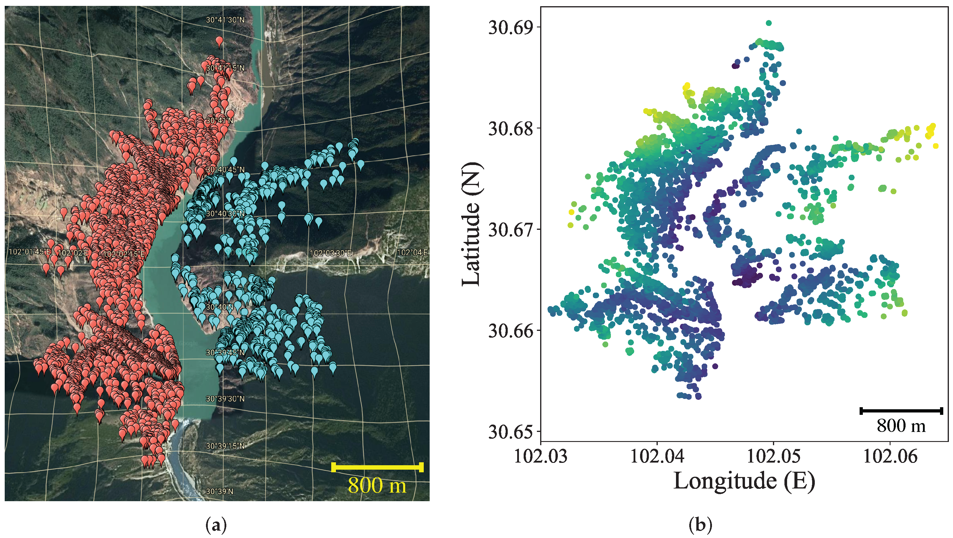
InSAR measurements: The data consists of N monitored sites , where is a particular site determined by 3D geographical coordinates (longitude, latitude, elevation). In each site, the displacement is measured by InSAR technology, and consists of a sequence of records representing the deformation of this monitored site evolving in time. The formula indicates each deformation that has p features. Figure 1 illustrates the studied slopes (details are described in Section 4).
Definition 1.
Land Displacement Prediction. Given the land graph and the corresponding historical displacement observations as inputs and as labels—where denotes the observations of all sites at time t, our objective is to learn a nonlinear regression model that outputs the predictions of all N locations over the next time steps:
3.2. LandGNN
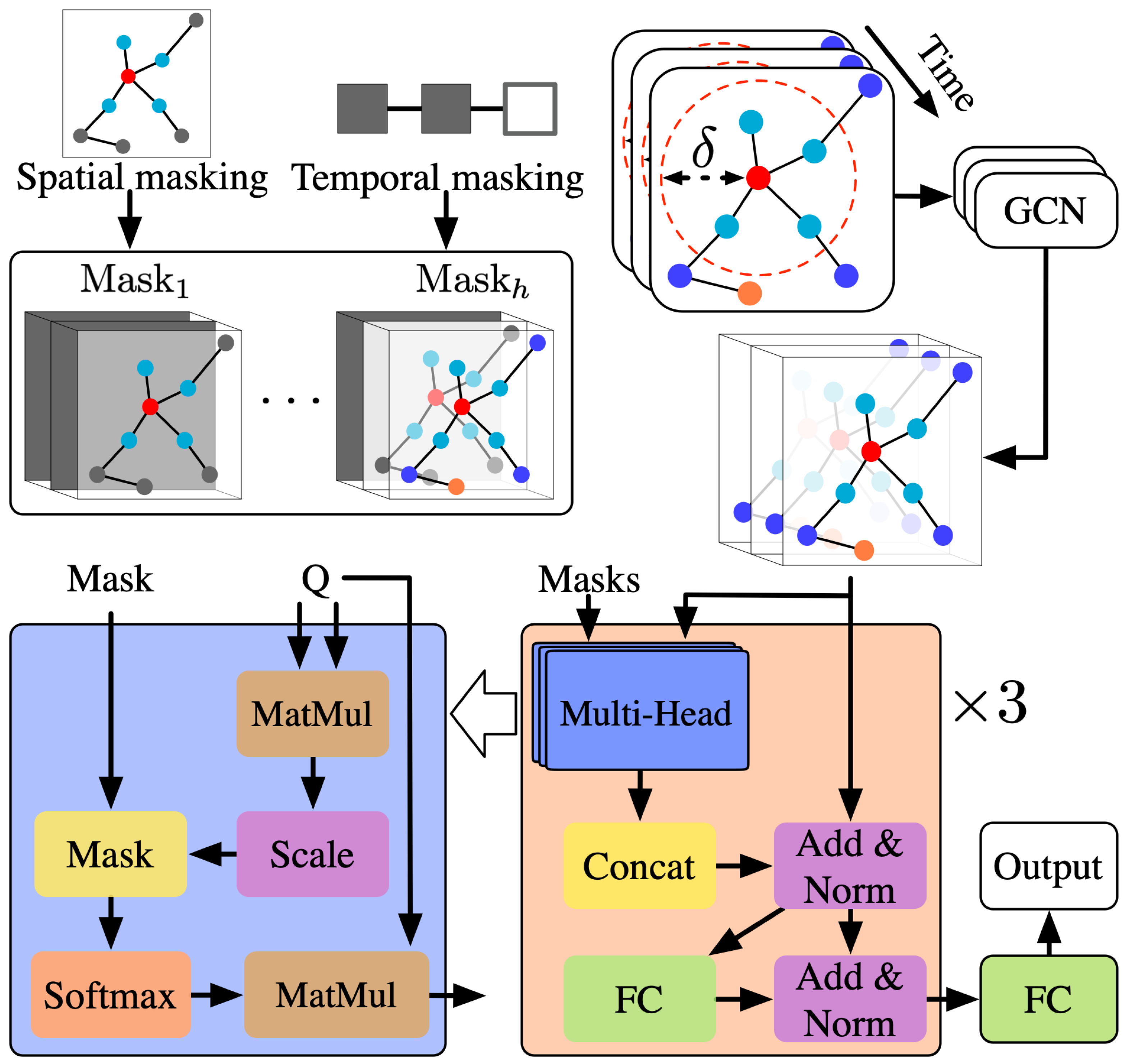
The main idea behind LandGNN is depicted in Figure 2. First, it builds the spatial graph containing neighborhood relations and geographical relative position relations. Next, we employ a typical graph convolution network to compute the feature fusion from neighbors. Subsequently, a locally historical Transformer is proposed to aggregate spatio-temporal features and make final predictions. With such architecture, LandGNN not only learns the intra-independence of nearing sites but also considers the evolution of local interactions.
3.2.1. Spatial Graph
Considering the InSAR data in different sites are independent of each other, the correlations among sites must be built into a spatial graph. Naturally, we can map original 3D relative positions to a graph, where nearing sites are closer to each other in Euclidean distance. A direct solution to the prediction problem is converting the point cloud into a 2D image from which CNNs can learn spatial features for prediction. However, the prediction accuracy is limited due to the image resolution and the information loss resulting from mapping the 3D point cloud to the 2D image. Recently, methods based on the 3D point cloud have enabled significant improvements [53]. By connecting near-neighbors within a pre-set fixed distance, graphs containing spatial correlations can be easily constructed. Building such a graph has been proven effective in object detection in computer vision. Following the same idea, we convert InSAR data into a graph. We set a threshold and then connect all sites pair and if Euclidean distance . Note that the threshold is a critical hyper-parameter, balancing the preservation of more geographical information with discarding redundant edges.
3.2.2. Spatial Feature Fusion
Catastrophic movement would result in dramatic changes to the surface, which are usually severe and would be quickly transmitted to adjacent areas. There is no site isolated from others on the surface, and the deformation will spread to surrounding locations, causing a more comprehensive range of surface changes. Therefore, there are signs that precede a massive landslide. We can continuously monitor the ground and give a warning when the range of deformation exceeds expectations. Toward this end, we apply convolution operations [47] over the graph to aggregate neighbors’ features and capture this kind of interaction:
where is the adjacency matrix, is the corresponding degree matrix, is the identity matrix and controls self-weight. is the input of y-th layer with trainable parameters , and we have Y layers in total. We initialize , and use ReLU as the activation function. Let and , where . Then Equation (2) can be rewritten as follows:
Right after the is defined, is fixed and used throughout the entire graph convolution procedure. Since the absolute values of deformation are generally far less than the geographical positions, we can approximately consider the graph as invariant during the monitored and predicted periods calculated in advance as a constant. Next, we obtain high-order features by applying Equation (3) recursively to aggregate from y-th order neighborhood. And we found that a 3-layer convolutional network is sufficient in our empirical evaluations, and we denote as feature fusion output. Note that many advanced GNNs such as GraphSAGE and GIN can be easily used to replace the GCN.
3.2.3. Locally Historical Transformer
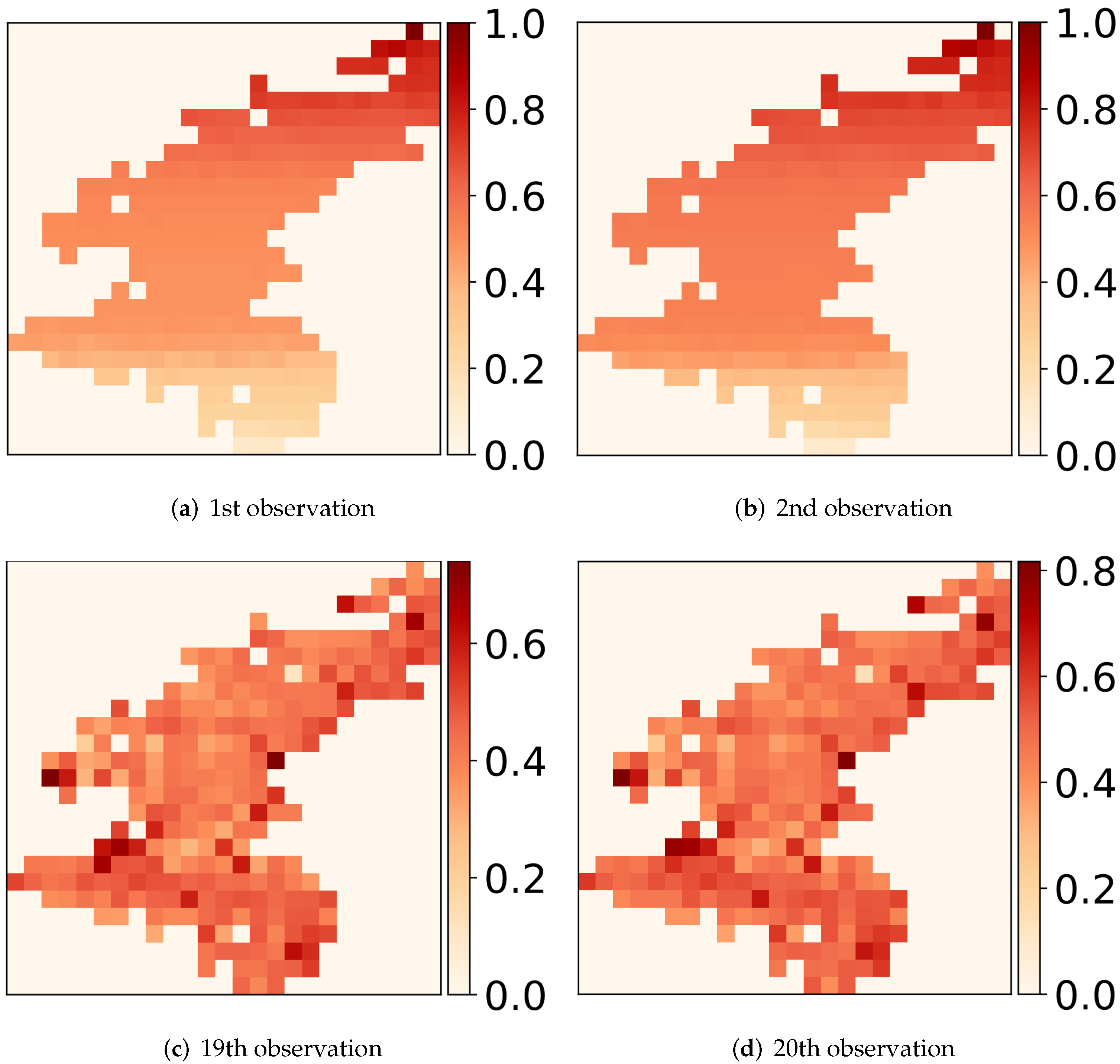
We draw some observations at different timestamps in Figure 3, in which the relative displacements are re-scaled from 0 to 1. We found that the displacements are consecutive both spatially and temporally. On the one hand, the displacements of sites at a specific time are very similar to observations at the previous time step. On the other hand, the deformations in spatially close areas are very similar and interact with each other. That is, spatio-temporal causality is critical for modeling and predicting landslide susceptibility.
Transformer architecture and attention mechanisms have been widely used for capturing spatial, temporal [48,61], and spatio-temporal dependencies [31,32,33]. However, existing methods use two groups of attention blocks to model spatial and temporal dependencies separately and then concatenate the results. As a result, these studies cannot exploit the full potential of self-attention to learn spatio-temporal correlations jointly. This motivates us to propose novel locally historical attention blocks to systematically explore the spatio-temporal causality. More specifically, we propose using spatio-temporal masks to encode corresponding positions that comprise positional information from both temporal and spatial perspectives. Multiple positional masks are applied in different attention heads to model multi-level spatial dependency.
Traditionally, we can build a triangular matrix to represent temporal dependency and a reachability matrix to represent spatial geographical dependency. Since the key is to guild locally historical mask—as illustrated in Figure 2, we propose a mask matrix to model spatial and temporal dependencies jointly, which can be formalized as:
where are k-hop neighbors of that can be found by k-hop accessibility matrix . The nodes marked by 0 will be ignored. Moreover, multi-head attention is utilized to handle the complexity of multi-reachability. is duplicated h times and sent to h heads, and in each processing we calculate a customized masking for k-hop reachability by Equation (4). With such a mask design, the attention blocks are able to model spatial and temporal dependencies concomitantly. Subsequently, we compute the self-attention block following [30] as:
where ⊙ is Hadamard product (i.e., element-wise matrix product), , , are matrices of queries, keys and values, respectively. Next, we concatenate h heads together:
where is trainable parameters that can aggregate features from attention heads and control the output size. Note that are not associated with h and can be determined by the necessity of the situation. One can use an arbitrary number of locally historical attention blocks to obtain the best performance.
The locally historical transformer can handle different adjacency matrices and spatio-temporal masks, allowing LandGNN to capture the dynamic spatio-temporal relationships and adapt to different locations. Note that many monitored areas may lead to space complexity explosion and attention weights dispersion. Therefore, in implementation, one can sample a subset of nodes, make predictions on the corresponding subgraphs iteratively, and calculate the average results at every location to approximate the predictions. Algorithm 1 summarizes the details of predicting land displacement via LandGNN.
| Algorithm 1 Predicting via LandGNN. |
Input: Adjacency matrix , reachability on h heads , N monitored sites S, displacement observations , convolution layers Y.
|
3.2.4. Objective
Given the ground-truth () and the predicted () displacement values of each node, we aim to minimize the gap between them as:
which is exactly the root mean square errors (RMSE).
4. Experiments
We now present the experimental results that demonstrate the effectiveness of LandGNN against the state-of-the-art landslide prediction algorithms.
4.1. Dataset
Our model and the baselines are evaluated on real-world InSAR data of the slopes around a large-scale hydropower station Houziyan Dam, located on the Dadu River in Danba County, Sichuan province, China. Figure 1a illustrates the studied slopes, where dots alongside the river denote the monitored locations—red and cyan dots denote areas on the west and east sides, respectively. Figure 1b plots the plain graph, where the color is darker, the lower the node is. For both slopes, we used eight months of data spanning from 1 January 2019 to 31 August 2019 for evaluations. Table 1 summarizes the statistics of the two slopes. Note that the land displacement on the east side is slightly larger.
4.2. Baselines and Experimental Settings
We compare our method against the following baselines: (1) Historical Average (HA) is a time series model that predicts the future displacement of each location according to the averaged previous observations; (2) Support Vector Regression (SVR) is a typical time-series model which predicts the value at a future time step through minimizing the generalization error bound [17]; (3) Autoregressive Integrated Moving Average (ARIMA) is one of the most consolidated statistics-based approaches for time series modeling and prediction; (4) LSTM and GRU are two well-known variants of RNN that have been used for time series prediction [62]; (5) STGCN utilizes temporal gated convolution to model time-series by an external specially designed graph and is wildly used for traffic prediction [27]; (6) DCRNN captures spatial features from random walks and temporal features from an auto-encoder structure [28]. (7) STAL is an attention-based LSTM for spatio-temporal forecasting [62].
All the models are trained on a server with a GeForce GTX 3090 GPU. We used the previous 50% observations for training and 30% data for validation. We then tested the models with the remaining 20% most recent data. HA, SVR and ARIMA are trained using the machine learning toolkit scikit-learn (https://scikit-learn.org). The deep learning models are tuned using Adam optimizer with an initial learning rate of 3 × 10. Both LSTM and GRU are 3-layer neural networks with 250 units in each layer. Our LandGNN is implemented with a 3-layer graph convolution network with 50 units in each layer. The spatially local transformer consists of a 3-layer decoder, and each layer has a 3-head attention block with 1, 2, and 3 order reachability matrices as masks. The graphs were built using thresholds for the west side, and for the east side, and the default self-connection weight of is 15.
4.3. Evaluation Metrics
We report the performance of all models using metrics widely used for evaluating time series models: RMSE, mean absolute error (MAE), accuracy (ACC), coefficient of determination (R), and explained variance score (EVS).
- Root Mean Squared Error (RMSE):
- Mean Absolute Error (MAE):
- Accuracy:
- Coefficient of Determination (R):
- Explained Variance Score (var):where and represent the true and predicted measurement at time and iff x is true. Threshold for determining the correct prediction is 0.01. , and are real deformations, predicted deformations and average deformations, respectively.
4.4. Overall Performance Comparison
Table 2 reports the prediction performance of all models on two sides in terms of five metrics. We can see that our proposed model LandGNN consistently outperforms other methods across both land sides. This result demonstrates that modeling spatial correlations among different sites is essential in predicting landslide susceptibility. In addition, traditional machine learning models such as HA, SVR, and ARIMA perform poorly due to their inability to capture non-linear interactions between locations. Meanwhile, RNN models are good at modeling long- and short-term dependencies in time-series and, therefore, significantly improve the prediction performance over traditional methods. However, the difference between them is trivial, and most importantly, they ignore the spatial interactions, which leads to inferior results compared to other spatio-temporal models. However, STGCN and DCRNN build spatio-temporal dependencies separately and sequentially compared to LandGNN, which models spatio-temporal dependencies as a whole, explaining the performance degradation. The comparison between STAL and LandGNN indicates that our model is superior to temporal prediction models, which verifies the contribution of the locally historical attention block. Moreover, our locally historical transformer network is better at capturing spatio-temporal dependency than vanilla GNN-based approaches such as STGCN and DCRNN.
4.5. Parameter Sensitivity
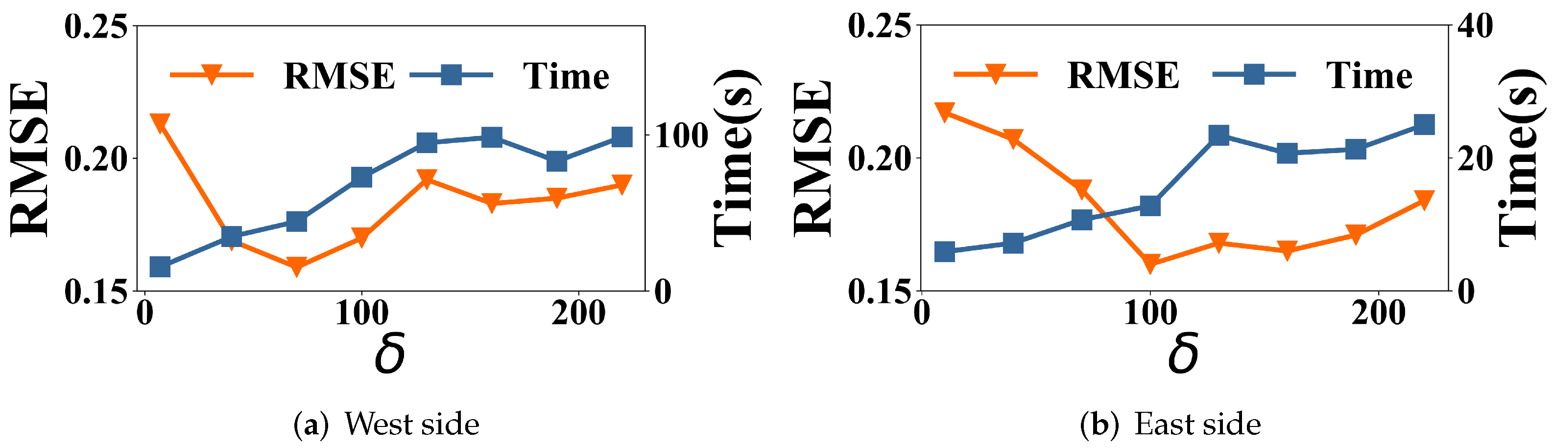
We now investigate the influence of two crucial hyperparameters in LandGNN. First, we discuss the influence of self-weight. Parameter determines how dense the constructed neighbor graph would be. Naturally, a more significant value of would result in a denser graph, requiring more computational cost for feature aggregation. Figure 4 shows how the prediction performance is affected by and its impact on training time. In the beginning, we hypothesized that the larger the value of , the better the prediction results. However, this hypothesis does not hold. For example, 80 m and 100 m are enough for the model to achieve the best performance on two sides. Therefore, increase the value of would degrade the model performance. This phenomenon happens due to the displacement nature of the lands. The surrounding areas may have similar displacements (e.g., positive values), which cannot be generalized to locations residing in distant places—where the displacements might be negative, which would neutralize the feature aggregations in GCN.
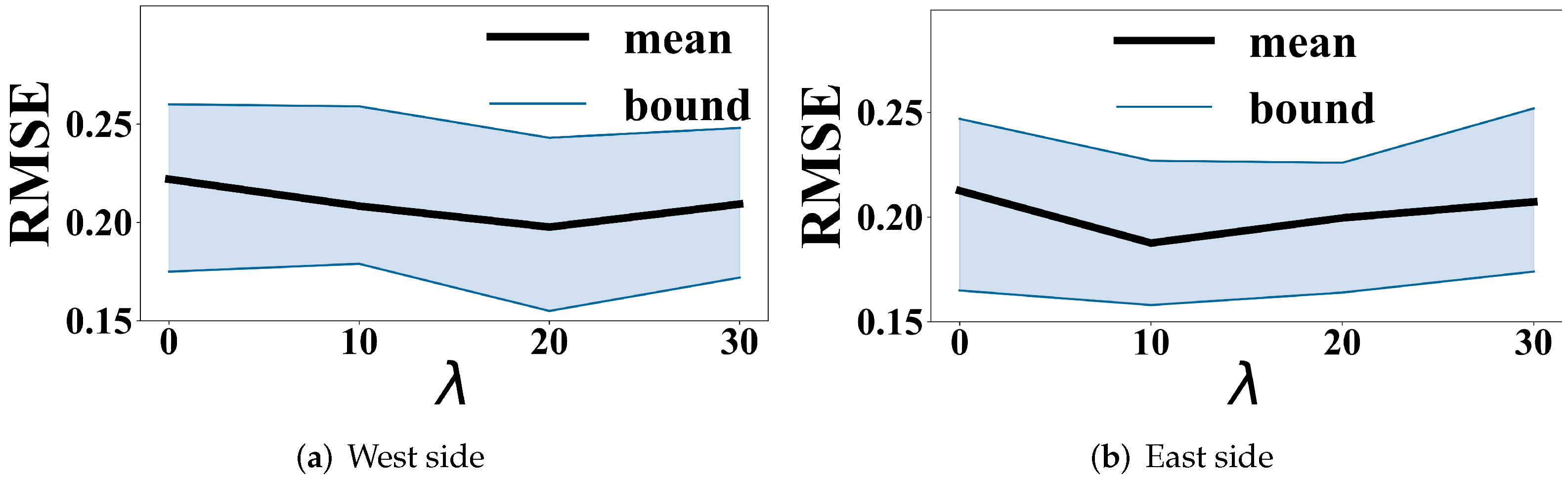
Another important hyperparameter is the distance threshold when constructing the adjacency matrix. When we consider more neighbors, the influence of the node itself decreases. For an aggregation network with a certain distance threshold , an optimal that controls the self-weight exists for the best prediction performance. Figure 5 shows the mean RMSE as well as the range of standard errors obtained from 10-run experiments. We can see that the optimal is around 20 and 10 for the west and east sides, respectively.
4.6. Visualizations
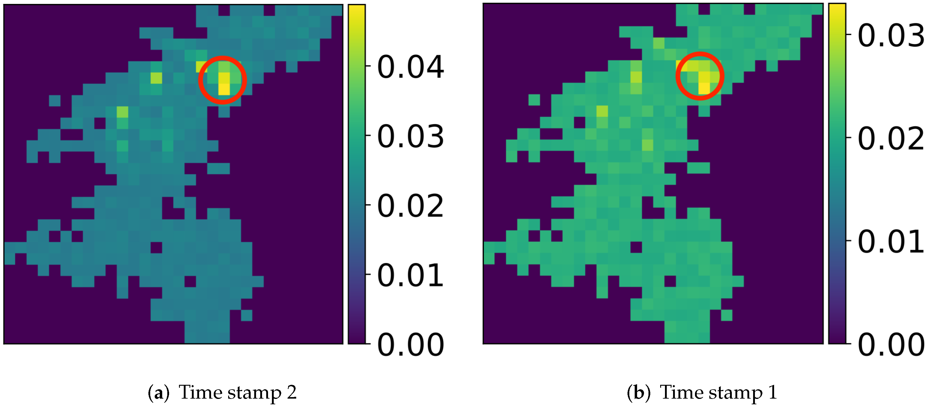
To explore how the proposed locally historical transformer works, we draw some attention weights of the first self-attention block in Figure 6. When making predictions at timestamp 3, we randomly select one location which lies precisely at the center of the red circle and draw its attention weights paid to locations on timestamps 2 and 1 with a 2-hop accessibility matrix. Additionally, to distinguish little attention weights and background, we set all pixel background values to 0. We also added 0.02 to pixels of all monitored locations so that the sum of their values is larger than 1. Results show that the predictions on the selected area are influenced mainly by neighboring areas with higher values of blocks. Moreover, the attention paid at timestamp 1 is less than at timestamp 2, which can be inferred by the scale of the color bar. In a word, attention is more densely distributed as monitored time is closer, which exactly confirms the motivation of our locally historical transformer, i.e., we should focus on more spatially and temporally relative locations in landslide forecasting.
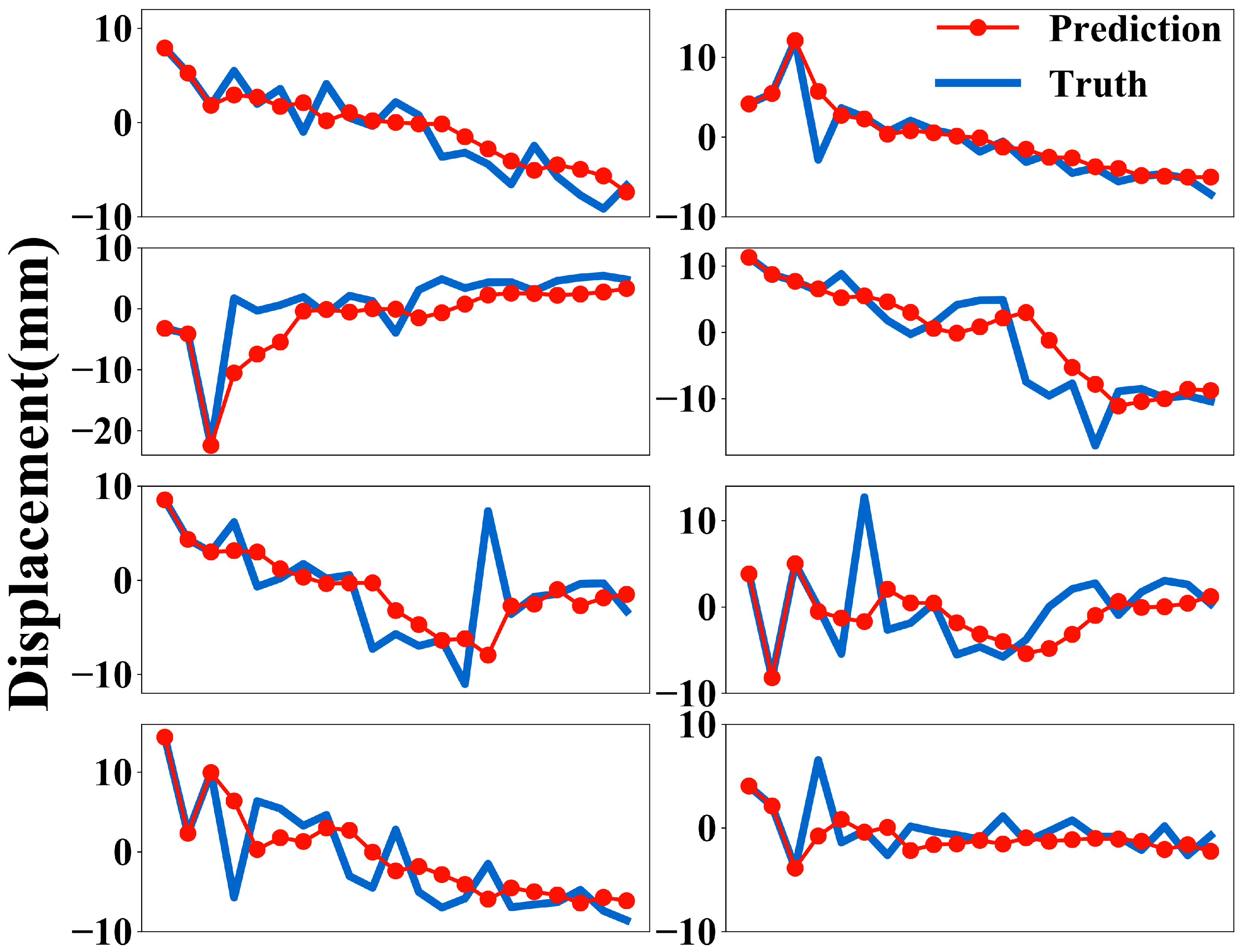
We also depict the real deformation and the predicted values to investigate the performance of LandGNN qualitatively. We randomly selected several monitored sites for visualization, and the results are shown in Figure 7. We can see that predictions made by LandGNN follow the actual displacement trend, indicating that our method can capture real-time landslide susceptibility.
5. Discussion
In the last section, we have empirically shown that LandGNN performs well in forecasting land displacement. We contrast the forecasting performance of LandGNN within three distinct groups of approaches, including statistic, machine learning, and deep learning methods. Experimental results under five evaluations are reported in Table 2, showing the superiority of LandGNN generally. In this section, based on the experimental results, we discuss both advantages and disadvantages of our model in comparison to the baselines and discuss what challenges we may face when deploying our model in the wild.
We observe that models solely rely on time-series perform worse than other spatio-temporal models. Although there is extensive evidence that modeling spatio-temporal dependencies is critical for forecasting tasks [27,28,62], we show that capturing spatio-temporal dependencies jointly can further improve the performance of our model. As shown in Figure 3, the displacements are consecutive spatially and temporally, which motivates us to design the locally historical transformer to handle the complicated interactions. The contrast of STAL and LandGNN strongly validates the effectiveness of the proposed mechanism and the re-modeling of standard transformers since both of them are attention-based. It also verifies the argument that modeling spatio-temporal dependencies jointly is a better approach. Though the proposed LandGNN combined with locally historical transformer outperforms baselines significantly, there is room for further improvements. For example, in addition to the joint modeling of spatio-temporal dependencies we designed in LandGNN, other fusing mechanisms can be used here to boost performance. Another potential improvement for LandGNN could be the computing efficiency (due to the expensive costs of monitoring landslides and real-time deformation computations). We think more efforts are desired to investigate efficient model structures while maintaining a satisfactory performance.
Another concern is about the adjacency matrix construction. The collected InSAR data are isolated 3D points with varying displacements, and most existing GNN approaches apply kNN or threshold approach to identify the neighbors of each point [27,50,51]. Following existing methods, we construct the proper adjacency relationships via searching the space of , as illustrated in Figure 4 of Section 4. After investigating different hyperparameter values, we determined the optimal for two datasets. We have discussed the potential reasons for performance improvement and degradation and how these hyperparameters possibly influence the subsequent aggregation mechanism, i.e., the GCN architecture in our case. It is also noteworthy that the performance of the LandGNN varies substantially within the threshold, which indicates that hyperparameter-tuning is indispensable in constructing a reliable forecasting system based on LandGNN. Since the threshold is not derivable, it usually requires a lot of human effort to tune the hyperparameters, especially when the dataset is large-scaled or in the circumstances that we need to re-train the model when we observe new InSAR data. On the other hand, the threshold-based adjacency matrix construction cannot model the complicated correlations among nodes because it is the only spatial distance we considered. In other words, dynamic adjacency matrices are desired for representing the varying node relationships. Therefore, we suggest three potential research directions for improving LandGNN: automatically discriminating neighbors for all nodes, mining the changing spatio-temporal correlations, and constructing a better adjacency matrix for feature aggregations.
Here we provide two more directions for future studies on landslide displacement prediction. First, the InSAR measurements are disturbed by the environment, and it inevitably brings noise to the data. That is to say, the correlations between nodes are usually uncertain. Existing models are still unable to learn data uncertainties and resist anomalies. We believe probabilistic approaches can be used here to make the model prediction more robust. Second, GNNs-based models often suffer from over-smoothing issues, and the suggested depth of GNN layers is generally no more than four layers. The intense displacements are therefore smoothed when aggregating the surrounding features, limiting the capabilities of transformers.
6. Conclusions
We presented LandGNN, a spatio-temporal graph neural network-based model for predicting land displacement using the high-quality InSAR measurement data.
- We apply graph convolution to aggregate spatial features on the defined graph structure and exploit transformer architecture to capture the locally historical dependencies between monitored nodes. Compared to traditional and deep learning-based methods, LandGNN explicitly models the spatio-temporal interactions between different locations and thus achieves better forecast performance.
- The experiments conducted on real-world datasets show that LandGNN is superior to previous approaches due to the capability of considering the evolution of local interactions. We also report the sensitivity of two important hyperparameters to explore the effectiveness of adjacency relations. Meanwhile, the visualization study indicates how the attention mechanism works, further validating our motivation.
- Our ongoing work aims to explore more information, such as the azimuth between monitored locations and the weather conditions to improve the accuracy and robustness of LandGNN. In addition, incorporating the data uncertainty and understanding the details of interactions between different areas while explaining the model prediction results are worthy of further investigation, which could benefit the development of prediction approaches useful for various safety-critical applications.
Author Contributions
Conceptualization, P.K., Y.H. and R.L.; methodology, R.L.; software, P.K. and Y.H.; validation, R.L., J.W. and F.Z.; formal analysis, J.W. and X.L.; investigation, P.K. and J.W.; resources, P.K. and Y.H.; data curation, R.L. and J.W.; writing—original draft preparation, R.L. and F.Z.; writing—review and editing, R.L., X.L., J.W. and F.Z.; visualization, R.L.; supervision, F.Z.; project administration, Y.H.; funding acquisition, P.K. and F.Z. All authors have read and agreed to the published version of the manuscript.
Funding
This work was funded by National Key R&D Program of China (Grant No.2019YFB1406202), National Natural Science Foundation of China (Grant No.62072077), and Sichuan Science and Technology Program (Grant No.2020YFG0234 and No.2020YFG0053).
Data Availability Statement
Not applicable.
Acknowledgments
This work was supported by National Key R&D Program of China (Grant No.2019YFB1406202), National Natural Science Foundation of China (Grant No.62072077), and Sichuan Science and Technology Program (Grant No.2020YFG0234 and No.2020YFG0053).
Conflicts of Interest
The authors declare no conflict of interest.
References
- Zhao, C.; Lu, Z. Remote Sensing of Landslides—A Review. Remote Sens. 2018, 10, 279. [Google Scholar] [CrossRef] [Green Version]
- Tsironi, V.; Ganas, A.; Karamitros, I.; Efstathiou, E.; Koukouvelas, I.; Sokos, E. Kinematics of Active Landslides in Achaia (Peloponnese, Greece) through InSAR Time Series Analysis and Relation to Rainfall Patterns. Remote Sens. 2022, 14, 844. [Google Scholar] [CrossRef]
- Huang, R.; Fan, X. The landslide story. Nat. Geosci. 2013, 6, 325–326. [Google Scholar] [CrossRef]
- Bozzano, F.; Cipriani, I.; Mazzanti, P.; Prestininzi, A. Displacement patterns of a landslide affected by human activities: Insights from ground-based InSAR monitoring. Nat. Hazards 2011, 59, 1377–1396. [Google Scholar] [CrossRef]
- Gao, W.; Dai, S.; Chen, X. Landslide prediction based on a combination intelligent method using the GM and ENN: Two cases of landslides in the Three Gorges Reservoir, China. Landslides 2020, 17, 111–126. [Google Scholar] [CrossRef]
- Hajimoradlou, A.; Roberti, G.; Poole, D. Predicting Landslides Using Locally Aligned Convolutional Neural Networks. In Proceedings of the International Joint Conference on Artificial Intelligence, Jokohoma, Japan, 7–15 January 2021; pp. 3342–3348. [Google Scholar]
- Liu, S.; Yin, K.; Zhou, C.; Gui, L.; Liang, X.; Lin, W.; Zhao, B. Susceptibility Assessment for Landslide Initiated along Power Transmission Lines. Remote Sens. 2021, 13, 5068. [Google Scholar] [CrossRef]
- Jiang, Y.; Luo, H.; Xu, Q.; Lu, Z.; Liao, L.; Li, H.; Hao, L. A Graph Convolutional Incorporating GRU Network for Landslide Displacement Forecasting Based on Spatiotemporal Analysis of GNSS Observations. Remote Sens. 2022, 14, 1016. [Google Scholar] [CrossRef]
- Gao, Y.; Chen, X.; Tu, R.; Chen, G.; Luo, T.; Xue, D. Prediction of Landslide Displacement Based on the Combined VMD-Stacked LSTM-TAR Model. Remote Sens. 2022, 14, 1164. [Google Scholar] [CrossRef]
- Kang, Y.; Zhao, C.; Zhang, Q.; Lu, Z.; Li, B. Application of InSAR Techniques to an Analysis of the Guanling Landslide. Remote Sens. 2017, 9, 1046. [Google Scholar] [CrossRef] [Green Version]
- Zhu, A.X.; Wang, R.; Qiao, J.; Qin, C.Z.; Chen, Y.; Liu, J.; Du, F.; Lin, Y.; Zhu, T. An expert knowledge-based approach to landslide susceptibility mapping using GIS and fuzzy logic. Geomorphology 2014, 214, 128–138. [Google Scholar] [CrossRef]
- Vakhshoori, V.; Zare, M. Landslide susceptibility mapping by comparing weight of evidence, fuzzy logic, and frequency ratio methods. Geomat. Nat. Hazards Risk 2016, 7, 1731–1752. [Google Scholar] [CrossRef]
- Zhou, J.W.; Lu, P.Y.; Yang, Y.C. Reservoir Landslides and Its Hazard Effects for the Hydropower Station: A Case Study. In Proceedings of the World Landslide Forum, Ljubljana, Slovenia, 30 May–1 June 2017; pp. 699–706. [Google Scholar]
- Gan, B.R.; Yang, X.G.; Zhou, J.W. GIS-based remote sensing analysis of the spatial-temporal evolution of landslides in a hydropower reservoir in southwest China. Geomat. Nat. Hazards Risk 2019, 10, 2291–2312. [Google Scholar] [CrossRef]
- Chen, W.; Xie, X.; Peng, J.; Wang, J.; Duan, Z.; Hong, H. GIS-based landslide susceptibility modelling: A comparative assessment of kernel logistic regression, Naïve-Bayes tree, and alternating decision tree models. Geomat. Nat. Hazards Risk 2017, 8, 950–973. [Google Scholar] [CrossRef] [Green Version]
- Wang, Q.; Wang, Y.; Niu, R.; Peng, L. Integration of Information Theory, K-Means Cluster Analysis and the Logistic Regression Model for Landslide Susceptibility Mapping in the Three Gorges Area, China. Remote Sens. 2017, 9, 938. [Google Scholar] [CrossRef] [Green Version]
- Kalantar, B.; Pradhan, B.; Naghibi, S.A.; Motevalli, A.; Mansor, S. Assessment of the effects of training data selection on the landslide susceptibility mapping: A comparison between support vector machine (SVM), logistic regression (LR) and artificial neural networks (ANN). Geomat. Nat. Hazards Risk 2018, 9, 49–69. [Google Scholar] [CrossRef]
- Hong, H.; Pourghasemi, H.R.; Pourtaghi, Z.S. Landslide susceptibility assessment in Lianhua County (China): A comparison between a random forest data mining technique and bivariate and multivariate statistical models. Geomorphology 2016, 259, 105–118. [Google Scholar] [CrossRef]
- Hong, H.; Pradhan, B.; Jebur, M.N.; Bui, D.T.; Xu, C.; Akgun, A. Spatial prediction of landslide hazard at the Luxi area (China) using support vector machines. Environ. Earth Sci. 2016, 75, 40. [Google Scholar] [CrossRef]
- Liu, R.; Peng, J.; Leng, Y.; Lee, S.; Panahi, M.; Chen, W.; Zhao, X. Hybrids of Support Vector Regression with Grey Wolf Optimizer and Firefly Algorithm for Spatial Prediction of Landslide Susceptibility. Remote Sens. 2021, 13, 4966. [Google Scholar] [CrossRef]
- Jiang, P.; Chen, J. Displacement prediction of landslide based on generalized regression neural networks with K-fold cross-validation. Neurocomputing 2016, 198, 40–47. [Google Scholar] [CrossRef]
- Ghorbanzadeh, O.; Blaschke, T.; Gholamnia, K.; Meena, S.R.; Tiede, D.; Aryal, J. Evaluation of different machine learning methods and deep-learning convolutional neural networks for landslide detection. Remote Sens. 2019, 11, 196. [Google Scholar] [CrossRef] [Green Version]
- Lei, T.; Zhang, Y.; Lv, Z.; Li, S.; Liu, S.; Nandi, A.K. Landslide inventory mapping from bitemporal images using deep convolutional neural networks. IEEE Geosci. Remote Sens. Lett. 2019, 16, 982–986. [Google Scholar] [CrossRef]
- Hua, Y.; Wang, X.; Li, Y.; Xu, P.; Xia, W. Dynamic development of landslide susceptibility based on slope unit and deep neural networks. Landslides 2020, 18, 281–302. [Google Scholar] [CrossRef]
- Dong, J.; Zhang, L.; Liao, M.; Gong, J. Improved correction of seasonal tropospheric delay in InSAR observations for landslide deformation monitoring. Remote Sens. Environ. 2019, 233, 111370. [Google Scholar] [CrossRef]
- Carlà, T.; Intrieri, E.; Raspini, F.; Bardi, F.; Farina, P.; Ferretti, A.; Colombo, D.; Novali, F.; Casagli, N. Perspectives on the prediction of catastrophic slope failures from satellite InSAR. Sci. Rep. 2019, 9, 1–9. [Google Scholar] [CrossRef] [Green Version]
- Yu, B.; Yin, H.; Zhu, Z. Spatio-temporal graph convolutional networks: A deep learning framework for traffic forecasting. IJCAI 2018, 3634–3640. [Google Scholar]
- Li, Y.; Yu, R.; Shahabi, C.; Liu, Y. Diffusion Convolutional Recurrent Neural Network: Data-Driven Traffic Forecasting. In Proceedings of the International Conference on Learning Representations (ICLR), Vancouver, BC, Canada, 30 April–3 May 2019. [Google Scholar]
- Wang, X.; Ma, Y.; Wang, Y.; Jin, W.; Wang, X.; Tang, J.; Jia, C.; Yu, J. Traffic flow prediction via spatial temporal graph neural network. In Proceedings of the Web Conference, Online, 20–24 April 2020; pp. 1082–1092. [Google Scholar]
- Vaswani, A.; Shazeer, N.; Parmar, N.; Uszkoreit, J.; Jones, L.; Gomez, A.N.; Kaiser, L.; Polosukhin, I. Attention is all you need. arXiv 2017, arXiv:1706.03762. [Google Scholar]
- Yuan, Z.; Liu, H.; Liu, Y.; Zhang, D.; Yi, F.; Zhu, N.; Xiong, H. Spatio-temporal dual graph attention network for query-poi matching. In Proceedings of the 43rd International ACM SIGIR Conference on Research and Development in Information Retrieval, Xi’an, China, 25–30 July 2020; pp. 629–638. [Google Scholar]
- Park, C.; Lee, C.; Bahng, H.; Tae, Y.; Jin, S.; Kim, K.; Ko, S.; Choo, J. ST-GRAT: A Novel Spatio-temporal Graph Attention Networks for Accurately Forecasting Dynamically Changing Road Speed. In Proceedings of the 29th ACM International Conference on Information & Knowledge Management, New York, NY, USA, 19–23 October 2020; pp. 1215–1224. [Google Scholar]
- Liu, J.; Guang, Y.; Rojas, J. Gast-net: Graph attention spatio-temporal convolutional networks for 3d human pose estimation in video. arXiv 2020, arXiv:2003.14179. [Google Scholar]
- Cui, W.; He, X.; Yao, M.; Wang, Z.; Hao, Y.; Li, J.; Wu, W.; Zhao, H.; Xia, C.; Li, J.; et al. Knowledge and Spatial Pyramid Distance-Based Gated Graph Attention Network for Remote Sensing Semantic Segmentation. Remote Sens. 2021, 13, 1312. [Google Scholar] [CrossRef]
- Liu, J.; Wu, Y.; Gao, X.; Zhang, X. A Simple Method of Mapping Landslides Runout Zones Considering Kinematic Uncertainties. Remote Sens. 2022, 14, 668. [Google Scholar] [CrossRef]
- Piacentini, D.; Troiani, F.; Torre, D.; Menichetti, M. Land-Surface Quantitative Analysis to Investigate the Spatial Distribution of Gravitational Landforms along Rocky Coasts. Remote Sens. 2021, 13, 5012. [Google Scholar] [CrossRef]
- Shirzadi, A.; Bui, D.T.; Pham, B.T.; Solaimani, K.; Chapi, K.; Kavian, A.; Shahabi, H.; Revhaug, I. Shallow landslide susceptibility assessment using a novel hybrid intelligence approach. Environ. Earth Sci. 2017, 76, 60. [Google Scholar] [CrossRef]
- Lizama, E.; Morales, B.; Somos-Valenzuela, M.; Chen, N.; Liu, M. Understanding Landslide Susceptibility in Northern Chilean Patagonia: A Basin-Scale Study Using Machine Learning and Field Data. Remote Sens. 2022, 14, 907. [Google Scholar] [CrossRef]
- Chung, J.; Gulcehre, C.; Cho, K.; Bengio, Y. Empirical evaluation of gated recurrent neural networks on sequence modeling. arXiv 2014, arXiv:1412.3555. [Google Scholar]
- Hochreiter, S.; Schmidhuber, J. Long short-term memory. Neural Comput. 1997, 9, 1735–1780. [Google Scholar] [CrossRef]
- Ju, Y.; Xu, Q.; Jin, S.; Li, W.; Su, Y.; Dong, X.; Guo, Q. Loess Landslide Detection Using Object Detection Algorithms in Northwest China. Remote Sens. 2022, 14, 1182. [Google Scholar] [CrossRef]
- Jepsen, T.S.; Jensen, C.S.; Nielsen, T.D. Relational fusion networks: Graph convolutional networks for road networks. IEEE Trans. Intell. Transp. Syst. 2020, 23, 418–429. [Google Scholar] [CrossRef]
- Hu, J.; Li, Z.; Ding, X.; Zhu, J.; Zhang, L.; Sun, Q. Resolving three-dimensional surface displacements from InSAR measurements: A review. Earth-Sci. Rev. 2014, 133, 1–17. [Google Scholar] [CrossRef]
- Osmanoğlu, B.; Sunar, F.; Wdowinski, S.; Cabral-Cano, E. Time series analysis of InSAR data: Methods and trends. ISPRS J. Photogramm. Remote Sens. 2016, 115, 90–102. [Google Scholar] [CrossRef]
- Solari, L.; Del Soldato, M.; Raspini, F.; Barra, A.; Bianchini, S.; Confuorto, P.; Casagli, N.; Crosetto, M. Review of Satellite Interferometry for Landslide Detection in Italy. Remote Sens. 2020, 12, 1351. [Google Scholar] [CrossRef]
- Ferretti, A.; Fumagalli, A.; Novali, F.; Prati, C.; Rocca, F.; Rucci, A. A New Algorithm for Processing Interferometric Data-Stacks: SqueeSAR. IEEE Trans. Geosci. Remote Sens. 2011, 49, 3460–3470. [Google Scholar] [CrossRef]
- Kipf, T.N.; Welling, M. Semi-Supervised Classification with Graph Convolutional Networks. In Proceedings of the International Conference on Learning Representations (ICLR), Toulon, France, 24–26 April 2017. [Google Scholar]
- Veličković, P.; Cucurull, G.; Casanova, A.; Romero, A.; Lio, P.; Bengio, Y. Graph Attention Networks. In Proceedings of the International Conference on Learning Representations (ICLR), Vancouver, BC, Canada, 30 April–3 May 2018. [Google Scholar]
- Wu, Z.; Pan, S.; Chen, F.; Long, G.; Zhang, C.; Philip, S.Y. A comprehensive survey on graph neural networks. IEEE Trans. Neur. Netw. Learn. Syst. 2020, 32, 4–24. [Google Scholar] [CrossRef] [PubMed] [Green Version]
- Han, J.; Liu, H.; Zhu, H.; Xiong, H.; Dou, D. Joint Air Quality and Weather Prediction Based on Multi-Adversarial Spatiotemporal Networks. In Proceedings of the 35th AAAI Conference on Artificial Intelligence, Virtual, 2–9 February 2021; pp. 4081–4089. [Google Scholar]
- Liu, J.; Li, T.; Ji, S.; Xie, P.; Du, S.; Teng, F.; Zhang, J. Urban flow pattern mining based on multi-source heterogeneous data fusion and knowledge graph embedding. IEEE Trans. Knowl. Data Eng. 2021. [Google Scholar] [CrossRef]
- Guo, S.; Lin, Y.; Wan, H.; Li, X.; Cong, G. Learning dynamics and heterogeneity of spatial-temporal graph data for traffic forecasting. IEEE Trans. Knowl. Data Eng. 2021. [Google Scholar] [CrossRef]
- Shi, W.; Ragunathan, R. Point-GNN: Graph Neural Network for 3D Object Detection in a Point Cloud. arXiv 2020, arXiv:2003.01251. [Google Scholar]
- Devlin, J.; Chang, M.W.; Lee, K.; Toutanova, K. Bert: Pre-training of deep bidirectional transformers for language understanding. arXiv 2018, arXiv:1810.04805. [Google Scholar]
- Brown, T.; Mann, B.; Ryder, N.; Subbiah, M.; Kaplan, J.D.; Dhariwal, P.; Neelakantan, A.; Shyam, P.; Sastry, G.; Askell, A.; et al. Language models are few-shot learners. NeurIPS 2020, 33, 1877–1901. [Google Scholar]
- Dosovitskiy, A.; Beyer, L.; Kolesnikov, A.; Weissenborn, D.; Zhai, X.; Unterthiner, T.; Dehghani, M.; Minderer, M.; Heigold, G.; Gelly, S.; et al. An Image is Worth 16×16 Words: Transformers for Image Recognition at Scale. In Proceedings of the International Conference on Learning Representations (ICLR), Virtual Event, 3–7 May 2021. [Google Scholar]
- Carion, N.; Massa, F.; Synnaeve, G.; Usunier, N.; Kirillov, A.; Zagoruyko, S. End-to-end object detection with transformers. In Proceedings of the European Conference on Computer Vision, Glasgow, UK, 23–28 August 2020; pp. 213–229. [Google Scholar]
- Liang, Y.; Zhou, P.; Zimmermann, R.; Yan, S. DualFormer: Local-Global Stratified Transformer for Efficient Video Recognition. arXiv 2021, arXiv:2112.04674. [Google Scholar]
- Guo, S.; Lin, Y.; Feng, N.; Song, C.; Wan, H. Attention based spatial-temporal graph convolutional networks for traffic flow forecasting. In Proceedings of the AAAI Conference on Artificial Intelligence, Honolulu, HI, USA, 27 January–1 February 2019; pp. 922–929. [Google Scholar]
- Cheng, W.; Shen, Y.; Zhu, Y.; Huang, L. A neural attention model for urban air quality inference: Learning the weights of monitoring stations. In Proceedings of the Thirty-Second AAAI Conference on Artificial Intelligence, New Orleans, LU, USA, 2–7 February 2018; Volume 32. [Google Scholar]
- Li, S.; Jin, X.; Xuan, Y.; Zhou, X.; Chen, W.; Wang, Y.X.; Yan, X. Enhancing the locality and breaking the memory bottleneck of transformer on time series forecasting. arXiv 2019, arXiv:1907.00235. [Google Scholar]
- Ding, Y.; Zhu, Y.; Feng, J.; Zhang, P.; Cheng, Z. Interpretable spatio-temporal attention LSTM model for flood forecasting. Neurocomputing 2020, 403, 348–359. [Google Scholar] [CrossRef]
Figure 1.
Multi-perspective views of the studied slopes. For Figure (a), the monitored locations on west and east slopes above the dam are marked as red and blue respectively; for Figure (b), the points are colored by elevation, and the lower the darker.
Figure 1.
Multi-perspective views of the studied slopes. For Figure (a), the monitored locations on west and east slopes above the dam are marked as red and blue respectively; for Figure (b), the points are colored by elevation, and the lower the darker.

Figure 2.
The framework of the proposed LandGNN.

Figure 3.
Heat map of displacements on 4 different days on west side.

Figure 4.
The influence of on computation time and prediction performance.

Figure 5.
The influence of .

Figure 6.
Attention weight distribution of a certain location (marked by red circle) on the west side.
Figure 6.
Attention weight distribution of a certain location (marked by red circle) on the west side.

Figure 7.
Prediction vs. the ground-truth.


Table 1.
Data description.
| Dataset | West Side | East Side |
|---|---|---|
| Nodes | 4569 | 2164 |
| Displacement range | [−27.58, 28.03] | [−29.06, 30.50] |
Table 2.
Performance comparison of displacement prediction on both sides of the river. For RMSE and MAE, the lower the value, the better the performance. Conversely, higher values are desirable for ACC, R and EVS.
Table 2.
Performance comparison of displacement prediction on both sides of the river. For RMSE and MAE, the lower the value, the better the performance. Conversely, higher values are desirable for ACC, R and EVS.
| Method | West Side | East Side | ||||||||
|---|---|---|---|---|---|---|---|---|---|---|
| RMSE | MAE | ACC | R | EVS | RMSE | MAE | ACC | R | EVS | |
| HA | 3.144 | 2.454 | 0.047 | 0.134 | 0.262 | 3.858 | 2.870 | 0.046 | 0.224 | 0.288 |
| SVR | 6.872 | 5.528 | 0.018 | 0.036 | 0.025 | 8.735 | 6.749 | 0.016 | 0.021 | 0.017 |
| ARIMA | 4.764 | 3.947 | 0.041 | 0.072 | 0.157 | 8.326 | 6.865 | 0.021 | 0.052 | 0.185 |
| LSTM | 0.254 | 0.218 | 0.490 | 0.038 | 0.094 | 0.254 | 0.210 | 0.518 | 0.077 | 0.086 |
| GRU | 0.254 | 0.217 | 0.491 | 0.040 | 0.095 | 0.250 | 0.207 | 0.526 | 0.078 | 0.092 |
| STGCN | 0.177 | 0.148 | 0.725 | 0.121 | 0.409 | 0.174 | 0.142 | 0.749 | 0.298 | 0.324 |
| DCRNN | 0.152 | 0.125 | 0.824 | 0.134 | 0.491 | 0.157 | 0.124 | 0.838 | 0.359 | 0.515 |
| STAL | 0.141 | 0.111 | 0.863 | 0.285 | 0.530 | 0.146 | 0.109 | 0.858 | 0.385 | 0.488 |
| LandGNN | 0.132 | 0.106 | 0.892 | 0.348 | 0.567 | 0.137 | 0.103 | 0.878 | 0.412 | 0.566 |
Publisher’s Note: MDPI stays neutral with regard to jurisdictional claims in published maps and institutional affiliations. |
© 2022 by the authors. Licensee MDPI, Basel, Switzerland. This article is an open access article distributed under the terms and conditions of the Creative Commons Attribution (CC BY) license (https://creativecommons.org/licenses/by/4.0/).
Share and Cite
MDPI and ACS Style
Kuang, P.; Li, R.; Huang, Y.; Wu, J.; Luo, X.; Zhou, F. Landslide Displacement Prediction via Attentive Graph Neural Network. Remote Sens. 2022, 14, 1919. https://doi.org/10.3390/rs14081919
AMA Style
Kuang P, Li R, Huang Y, Wu J, Luo X, Zhou F. Landslide Displacement Prediction via Attentive Graph Neural Network. Remote Sensing. 2022; 14(8):1919. https://doi.org/10.3390/rs14081919
Chicago/Turabian StyleKuang, Ping, Rongfan Li, Ying Huang, Jin Wu, Xucheng Luo, and Fan Zhou. 2022. "Landslide Displacement Prediction via Attentive Graph Neural Network" Remote Sensing 14, no. 8: 1919. https://doi.org/10.3390/rs14081919
Note that from the first issue of 2016, this journal uses article numbers instead of page numbers. See further details here.