An Attention Cascade Global–Local Network for Remote Sensing Scene Classification

Abstract

Remote sensing image scene classification is an important task of remote sensing image interpretation, which has recently been well addressed by the convolutional neural network owing to its powerful learning ability. However, due to the multiple types of geographical information and redundant background information of the remote sensing images, most of the CNN-based methods, especially those based on a single CNN model and those ignoring the combination of global and local features, exhibit limited performance on accurate classification. To compensate for such insufficiency, we propose a new dual-model deep feature fusion method based on an attention cascade global–local network (ACGLNet). Specifically, we use two popular CNNs as the feature extractors to extract complementary multiscale features from the input image. Considering the characteristics of the global and local features, the proposed ACGLNet filters the redundant background information from the low-level features through the spatial attention mechanism, followed by which the locally attended features are fused with the high-level features. Then, bilinear fusion is employed to produce the fused representation of the dual model, which is finally fed to the classifier. Through extensive experiments on four public remote sensing scene datasets, including UCM, AID, PatternNet, and OPTIMAL-31, we demonstrate the feasibility of the proposed method and its superiority over the state-of-the-art scene classification methods.

1. Introduction

The cost of obtaining high-resolution remote sensing images is dramatically decreased with the continuous progres of satellite sensors and earth observation technology, along which more and more research attention is paid to the field of remote sensing. As one of the important topics, remote sensing scene classification recognizes the contents of remote sensing images with semantic labels and can be widely applied in land use, urban planning, environmental monitoring, natural disaster monitoring, etc.

The factors, such as abundant spatial texture features, various scenes, and complicated surface information, bring great challenges to scene classification with high-resolution remote sensing images [1]. At this regard, it is important to extract effective features from the complex image contents, which attracts different kinds of solutions. The feature extraction methods can be categorized as manual features and deep features. The former, such as color histogram (CH) [2] and scale-invariant feature transform (SIFT) [3], are easy to implement but highly depend on the priori knowledge of the designer, resulting in the features with low-level semantics and limited representational capacity. By contrast, the later benefit from the popularity of deep learning, especially the convolutional neural networks (CNNs), and produce the features in a data-driven manner without the need of priori knowledge of the designer. The resultant features possess high representational capacity, hence they are able to distinguish semantic features from complex scenes.

Remote sensing scene classification has exhibited success based on the classical CNN such as AlexNet [4], VGG-Net [5], GoogLeNet [6], and ResNet [7]. While the depth of a single could be an indicator of the classification performance, the model ability is upper-bounded by a certain depth and a deeper model cannot yield higher performance because of the limited training data and other unexplainable reasons. Considering that different deep models may have different perferences on feature extraction, i.e., the extracted features exhibit different characteristics, all these features could be partially complementary to each other. Hence, this motivates us to employ more than one models, which could be fused to improve the feature representation. The existing fusion methods for dual CNN model is realized by feature connection or dot production [8]. However, we argue that this simple fusion strategy is insufficient to exploit the dominant features of both models. Instead, we develop an advanced fusion method based on bilinear fusion, which produces a representative vector for the dual models, resulting in sufficient fusion of eigenvectors.

Moreover, the remote sensing images have a great difference compared with the natural images subject to the imaging height and the background complication. As shown in the airport scene in Figure 1, the interested objects indicated by the red boxes, i.e., the airplanes, distributed widely in the whole image. This inform us that the scene classification should focus on both local and global features [9,10,11]. The existing works have ignored abundant background information in the low-level semantics; the resultant features are hence not distinguishable enough to reach accurate classification. Targeting at this issue, we apply special attention models to exact global semantic information from the high-level features, which are fed back to the low-level information to enhance the local features of the salient regions and to reduce the background interference. Meanwhile, cross-layer feature fusion is considered to combine the features of different scales, which promotes feature propagation and feature reuse in forward propagation. Taking all the above discussions into consideration, we develop an attention cascade global–local network (ACGLNet) that exploits the local features, the global features, the multiscale features, and the dual-model features via elaborated fusion schemes and achieves superior classification performance over the state-of-the-art methods.

The major contributions of this paper are summarized as follows:

(1) A novel ACGLNet model is proposed. The ACGLNet is equipped with an elaborated deep feature fusion strategy based on multiscale and multimodel features. The proposed model brings higher performance of scene classification than the competitors on several public datasets.

(2) Targeting the tiny targets and the complex background of remote sensing images, we propose to fully integrate the global and local features to depress the redundant background information in low-level features and combine the effective low-level features with high-level features. In this way, the resultant feature can be resistant to the influence of complex and redundant backgrounds.

(3) We propose to combine the dual-model features by bilinear fusion, which can capture the production relationships within all elements in two eigenvectors to obtain sufficient fusion at the pixel level.

The rest of this paper is organized as follows. Section 2 reviews the related work, including the research on remote sensing image scene classification and the attention mechanisms. Section 3 describes our proposed method in details. In Section 4, experimental results and analyses on several public scene datasets are presented. The empirical comparison between the proposed method and the state-of-the-art methods is conducted in Section 5. Finally, the conclusion is drawn in Section 6.

2. Related Work

In this section, we briefly review the recent literature about the remote sensing image scene classification and the attention mechanism.

(1) Remote Sensing Image Scene Classification Methods

Scene classification on remote sensing images has great value in a variety of fields such as object detection, homeland planning, and disaster detection. The current scene classification methods can be classified into two categories—those based on traditional features [12] and those based on deep features [13].

In the early years, researchers focused on the traditional features, which were generally shallow features developed based on the prior knowledge about remote sensing images, such as lights, colors, textures, and shapes. These methods included the grey-level cooccurrence matrix [14], the histograms of oriented gradients [15], and the Gabor filters [16], which were easy to implement. However, the main drawback stated that each single feature was insufficient for representing the high-level semantic information, hence leading to a low accuracy of classification. These features were usually combined to integrate multiple kinds of information, yielding improved performance [17]. However, these methods based on traditional features were not suitable for classifying the scenes with complicated backgrounds due to their limited representative capability.

With the development of deep learning, scene classification has benefitted greatly from the popular deep models, such as the stacked autoencoder (SAE) [18], the deep belief network (DBN) [19], and the convolutional neural networks (CNNs) [20]. For instance, Xing et al. [21] applied SAE on the task of scene classification on remote sensing images. Yang et al. [22] established a four-layer DBN to extract semantic features. As the most popular architecture, the CNN models, which possess strong representative capability and generalization ability, have produced promising performance compared with other architectures [23]. Yuan et al. [24] proposed a strategy based on spatial similarity to rearrange the local features extracted by the pretrained VGG19Net for scene classification. Castelluccio M et al. [25] applied the pretrained GoogleNet model for land classification. Nogueira et al. [26] integrated the linear supported vector machine (SVM) into CNN to extract global information directly. Han et al. [27] proposed a semisupervised generative framework (SSGF), which combined deep features, self-labeling, and discriminant evaluation. Meanwhile, the CNN methods combined with the traditional features can also improve the representative capability [28,29,30,31]. For instance, the multiscale deep features processed by BoVW and Fisher encoder could be used to characterize the global feature space [28]. Liu et al. [29] combined the features of different pretrained CNN models to represent scene images. The models with different layers were also considered [30]. A probabilistic fusion model was also proposed with three different sizes of receptive fields [31].

(2) Attention Mechanism

The idea of attention mechanism originates from human vision. Since the capability of focusing on the whole visual field is limited, humans tend to focus on some specific regions to obtain the detailed information. This helps to filter the useless information and to improve the efficiency of processing [32]. Attention mechanisms set higher weights to the critical features so that the models can learn important regions in the image. Attention mechanisms are mainly divided into soft attention and hard attention. The former focuses on regions and channels. It is a differentiable deterministic mechanism, which can calculate the gradients and backpropagate the weights of attention during learning. The latter pays more attention to the points in images, which emphasizes dynamic changes with uncertainty. Compared to hard attention, soft attention is easier to train and thus has higher popularity [33,34]. Soft attention can be classified as spatial attention, channel attention, and mixed attention, such as spatial transformer network (STN) [35], squeeze and excitation network (SENet) [36], and residual attention network (RAN) [37]. In recent work, researchers have attempted to improve the accuracy of scene recognition tasks by allowing CNNs to reweight key features through attention mechanism. Wang et al. [38] proposed a novel end-to-end attention convolutional networks (ARCnet) for scene classification. Tong et al. [39] introduced the channel attention mechanism into DenseNet [40] and proposed a channel-attention-based DenseNet (CAD) [41]. Spatial attention was introduced to shallow features while channel attention was added to deep features, which resuled in a novel Saliency Dual Attention Residual Network (SDAResNet) [42]. Fan et al. [43] proposed a CNN-based network with residual and attention model, which could automatically assign large weights for important features and ignore redundant information.

Generally speaking, the traditional features have limited representative capability, which are not suitable for complex feature modelling problems. This is to say that these methods have insufficient generalization ability and robustness, which is nevertheless critical for classifying complicated scenes. With the assistance of deep features, these issues can be alleviated since the deep models can learn semantic information adaptively to improve the representative capability, resulting in pleasing classification accuracies. Feature fusion can also enhance the feature distinguishability. While attention mechanism has been successfully introduced into scene classification of remote sensing images, most of the previous works regard the fully connected layers as global features and ignore the local features. Instead, the proposed ACGLNet can extract both global and local features simultaneously to improve the classification accuracy.

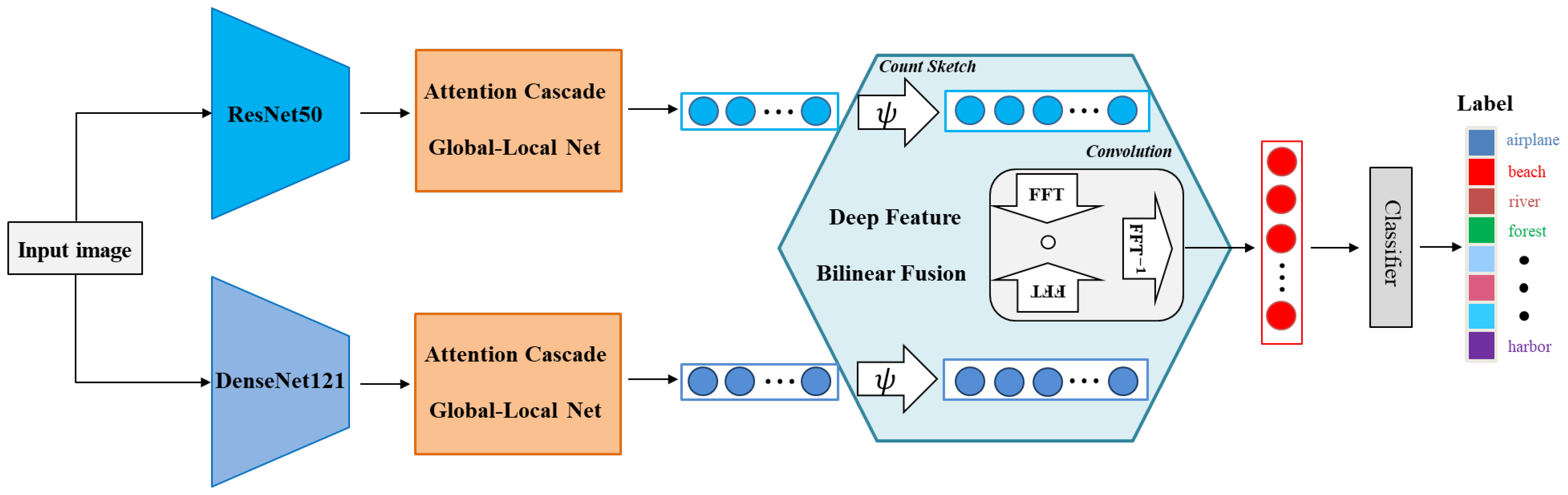
3. The Proposed Method

The overall structure of our proposed method is depicted in Figure 2. The key idea is to employ two different CNNs to extract complementary features which are then fused for feature enhancement. Each model produces the features under four different scales. The proposed ACGLNet helps each model to produce the image representation by effectively integrating the global and local features. Then, we obtain the dual-model fused representation through the deep feature bilinear fusion method. This representation is finally fed to the classifier to produce the classification result.

3.1. Feature Extraction

To solve the problem that a single CNN has the lack of feature extraction capability, we propose a structure with dual CNN models. Here, we choose two representative CNN models, namely ResNet and DenseNet, as the feature extractors. The details are introduced as follows.

(1) ResNet

The most outstanding characteristic of ResNet is the residual block, which extracts features from both the middle layers and the input layer through shortcut, thus avoiding the issues of gradient explosion and gradient vanishing. We choose ResNet50 as the basic feature extractor and set the output of $conv2\_x$, $conv3\_x$, $conv4\_x$, and $conv5\_x$ layers as the outputs in different scales.

(2) DenseNet

DenseNet is a large and intensive network that possesses a reduced number of parameters and produces improved features. Each layer takes the output of the previous layer as input and passes its corresponding feature mapping to all subsequent layers. This network can efficiently transport features to the deep layers, promoting the network to extract global and significant features. We choose DenseNet121 as another extractor and use Dense Block (1)–(4) as the features in four different scales.

3.2. Attention Cascade Global-Local Net (ACGLNet)

Since remote images are complicated in the background and the key objects are easily scattered, accurate scene classification should consider both global and local features, which may correspond to the high-level and low-level features, respectively. The low-level features contain the details of spatial structures, which remedy the losed spatial information in high-level features. Meanwhile, the high-level features may contain redundant background information, which interferes with the location of targets. By taking the advantages of both types of features, therefore, we propose a novel ACGLNet based on the pyramid structure [44], where the structure is illustrated in Figure 3. The higher-level features are used to generate the spatial attention map, which adaptively assigns weights to the corresponding locations of the lower-level features, depressing the irrelevant information of background. After fusing the weighted low-level and high-level features from the top to bottom through the pyramid, we add cross-scale cascade to obtain multiscale features with rich spatial and semantic information. Finally, we average the multiscale features to get the final output. In this way, the useful features in the input image are expected to be fully extracted while the information loss is minimized.

The spatial attention module is to enable the model to locate the region of interest in the input scene images while suppressing redundant noise interference [45]. The structure is shown in Figure 4. To exploit the attention strategy from high-level features, we establish a feature pyramid based on the features of the CNNs in four different scales, which are denoted as $\{C_2,C_3,C_4,C_5$ }. We first upsample the feature map $C_5$ by n times (n = 2, 4, 8) to match the size of each low-level feature map. Then, we apply two convolutional kernels with the sizes of $1\times 3$ and $3\times 1$ to extract semantic information from the previous stage. Two feature mappings are summed and then passed through a sigmoid function to produce a normalized spatial attention map with the size of $H\times W\times 1$, where H and W are the height and weight of the feature map, respectively. At last, the spatial attention map generated by the higher-level feature map is directly applied to the adjacent lower-level feature map, where the formula is expressed as: $F_l=C_A·C_l$, l = 2, 3, 4, where $C_A$ represents the spatial attention map created by $C_5$, $C_l$ denotes the low-level feature maps, and $F_l$ is the weighted low-level features with spatial attention.

Based on the definition of the feature pyramid module, we can get $\{F_2,F_3,F_4,C_5\}$, where $F_l$ denotes the weighted feature map with spatial attention. These four feature maps with different scales are first processed according to the architecture in Figure 3, generating the feature maps $\{P_2,P_3,P_4,P_5\}$. We double the size of each $P_l$ via upsampling, leading to the feature map with the same size as $F_{l-1}$. Then, $P_{l-1}$ is obtained by concatenating the upsampled feature map and $F_{l-1}$. In this way, the generated $\{P_2,P_3,P_4,P_5\}$ have the same size as $\{F_2,F_3,F_4,C_5\}$, respectively. All the feature maps are fused by a cross-layer cascade operation, which creates a mapping from the high-level feature maps $P_4,P_5$ to the low-level feature maps $P_2,P_3$ such that the semantic information for discrimination is improved. By this manner, a direct feature mapping from low-level features to high-level features is established. Figure 5 presents the procedure of cross-scale cascade.

The previous process can be presented as:

$$P_l=\left\{\begin{array}{cc}\hfill & Con{v}_{3\times 3}\left(Con{v}_{1\times 1}\right)\left(C_l\right)),l=5\hfill \\ \hfill & Con{v}_{3\times 3}(Upsample\left(P_{l+1}\right)\oplus Con{v}_{1\times 1}\left(F_l\right)),l=4\hfill \\ \hfill & Con{v}_{3\times 3}(\sum _{i=l+1}^{5}Upsample\left(P_i\right)\oplus Con{v}_{1\times 1}\left(F_l\right)),l=2,3\hfill \end{array}\right.$$

(1)

where $P_l$ is the processed feature map corresponding to one of $\{F_2,F_3,F_4,C_5\}$, $Con{v}_{k\times k}(·)$ denotes the convolutional operation with k-sized kernels, $Upsample(·)$ represents the upsampling operation, and ⊕ is the cascading operation. Note that we have applied $1\times 1$ convolution to reduce the dimension of $F_l$ (l = 2, 3, 4), such that the postprocessings can be efficient. The aliasing effect is eliminated by $3\times 3$ convolutional kernels in each layer of the feature pyramid.

Based on the feature pyramid, we then fuse the multiscale features as follows. We rescale $\{P_2,P_3,P_4,P_5\}$ to the size of $P_4$ via max-pooling or interpolation, resulting in the feature maps $\{N_2,N_3,N_4,N_5\}$. This helps the features in different layers to possess identical positional correspondence and semantic correspondence. Then, we can take the average to obtain the fused feature $N_m$, which is computed as

$$N_m=\frac{1}{L}\sum _{l=l_{min}}^{l=l_{max}}{N}_l$$

(2)

where L denotes the number of feature layers, $N_i$ refers to the feature in the lth layer, and $l_{min}$ and $l_{max}$ represent the indices of the lowest and highest layers, respectively. The global feature of $N_m$ can be calculated by

$$N_m=\frac{1}{H\times W}\sum _{i=1}^H\sum _{j=1}^W{N}_{i,j}^l$$

(3)

where $N^l\in R^{H\times W}$ denotes the lth channel of $N_m$, whose size is $H\times W$.

Finally, we obtain the global deep features $N_{c_1}\in R^{d_1}$ and $N_{c_2}\in R^{d_2}$ of the two models.

3.3. Deep Feature Bilinear Fusion

Considering the high complexity of remote sensing images, we fuse the deep features of the dual models to involve more abundant scene information and to increase the classification accuracy. The traditional feature fusion methods are based on either the serial strategy or the parallel strategy. The serial method directly connects two sets of features, where the dimension of the fused features equals the addition of the dimensions of the two features. The parallel strategy combines the features as a complex vector, i.e., $F_f=F_1+i{F}_2$, where $F_1$ and $F_2$ are input features and i is the complex unit.

These feature fusion methods, however, are unable to sufficiently use the input features, leading to an unsatisfactory representative capability and failing to capture complicated connections between these CNNs. Different from the previous two methods, bilinear pooling captures the production of all elements in the two vectors, which has recently revealed the availability in fine-grained visual recognition tasks [46]. An issue states that the bilinear pooling layer involves outer production, which increases the dimension and the computational complexity. Therefore, inspired by [47], we apply the deep feature bilinear fusion in our model. First, the Count-Sketch function is introduced to map the outer production of two vectors into a lower-dimensional space. Then, the outer production in the time domain is transformed into the dot product of the convolution of the two vectors in the frequency domain via fast Fourier transform (FFT). This avoids the problem of dimensional expansion caused by outer production.

Specifically, Count-Sketch function is involved to handle two global deep feature vectors $N_{C_1}$ and $N_{C_2}$ denoted as $\psi (N_{C_1}\otimes N_{C_2},h,s)$, where h and s are hash mapping. The Count Sketch of the outer product of two vectors can be expressed as the convolution of the respective Count Sketch [48], which is written as

$$\psi (N_{C_1}\otimes N_{C_2},h,s)=\psi (N_{C_1},h,s)\ast \psi (N_{C_2},h,s)$$

(4)

where ⊗ is the outer production and * is the inner production. In this way, we can approximately calculate the final fused feature of the dual models.

First, we initialize two vectors $h_k\in {\{1,2,\cdots ,d\}}^C$ and $s_k\in {\{-1,1\}}^C$, k = 1, 2. As for the indices of the input vector i, $s_k\left[i\right]$ equals to 1 or −1. $s_k$ and $h_k$ follow the uniform distribution on $\{-1,1\}$ and $\{1,2,\cdots ,d\}$, respectively. $h_k$ maps each index i of the input vector $N_{C_i}$ to the index $j\in \{1,2,\cdots ,d\}$ of the output vector, which is denoted as $j=h_k\left[i\right]$. The index j of the output vector satisfies

$$N_{c_k}^{\prime }\left[j\right]=N_{c_k}^{\prime }\left[h_k\left[i\right]\right]=\sum s_k\left[i\right]·N_{c_k}\left[i\right],i=1,2\cdots C$$

(5)

In this way, $N_{c_1}^{\prime },N_{c_2}^{\prime }\in R^d$ is the output vector obtained by the Count Sketch function $\psi$.

Finally, according to the product in the frequency domain corresponding to the convolution in the time domain, the fused feature $\varphi (N_{c_1},N_{c_2})\in R^d$ is obtained by

$$\begin{array}{c}\psi (N_{c_1}\otimes N_{c_2},h,s)=\varphi (N_{c_1},N_{c_2})\hfill \\ =FF{T}^{-1}(FFT\left(N_{c_1}^{\prime }\right)\circ FFT\left(N_{c_2}^{\prime }\right))\hfill \end{array}$$

(6)

where ∘ is dot production.

4. Experiments

In this section, we conduct comprehensive experiments and analysis on four general public scene classification datasets to validate the feasibility of our classification model. We first introduce these datasets and the experimental settings. Then, we quantitively compare the performance differences between our method and several state-of-the-art methods.

4.1. Datasets

(1) UC Merced Land-Data Set [49]: This dataset is collected by United States geological survey, (USGS), which has 21 scenes, including agriculture, airplane, storage tank, etc. Each class consists of 100 images with the size of $256\times 256$, and the pixel resolution is 0.3 m. UCM data set have the least number of scene categories, and the differences between the categories are more obvious.

(2) Aerial Image Data Set(AID) [50]: This is a large dataset for aerial scene image classification. It contains 30 categories, namely bare land, railway station, resort, etc. 10,000 images are involved, with 220 to 420 per category. Each image has the size of $600\times 600$, and the pixel resolution ranges from 1 m to 8 m.

(3) PatternNet [51]: This dataset is created by Wuhan University via Google Earth and Google Map API. It contains 38 classes, namely chaparral, Christmas tree farm, coastal mansion, etc. Each type of scene in this dataset contains 800 images, 30,400 images in total, with a size of $800\times 800$ pixels and the resolution of about 0.062 m to 4.693 m.

(4) OPTIMAL-31 Data Set [38]: All images in this dataset are collected from Google Earth. The dataset contains 31 categories and a total of 1860 images, where each category is composed of 60 images with the size of $256\times 256$. The categories in this dataset are circular farmland, ground track field, rectangular farmland, etc. This dataset contains more abundant information; thus, it is more difficult.

4.2. Evaluation Metrics

We apply the overall accuracy (OA) and the confusion matrix as the measurement of the algorithms.

(1) OA is defined as the number of the correct predictions divided by the whole number, reflecting the performance of whole classification.

(2) Confusion matrix presents more detailed information within each class. Each column refers to the predicted class while each row refers to the ground-truth class, and the diagnosis is the classification accuracy on each class.

4.3. Experimental Setups

(1) Training Details

For the UC Merced Land-Use Dataset, we set the training ratio to 50% and 80%, respectively, and the rest is used for testing. For the AID dataset and the PatternNet dataset, the training ratio is set to 20% and 50%, respectively. The training ratio is set to 80% for the OPTIMAL-31 Data Set. All images are rescaled to the size of $224\times 224$. In model training, we augment the data by random shifting, rotating, and flipping to increase the data diversity.

We choose ResNet-50 and DenseNet-121 as two backbones for feature extraction and use the pretrained weights from ImageNet to accelerate the training process. We apply the momentum-based stochastic gradient descent algorithm for optimization, where the momentum value is set to 0.9 with a decay parameter of 0.009. The learning rate is initialized as 0.001, which shrinks 10 times after every 100 epochs. All experiments are implemented with the PyTorch framework, on a device of Intel(R) Core(TM)i7-8700 CPU, 16 GB RAM, and an 11 GB NVIDIA GeForce GTX 1080Ti GPU.

(2) Parameter Settings

Our proposed model introduces a parameter d, namely the fusion dimension. It measures the useful information among features, reflecting the distinguishability. The ablation study is presented in

Table 1. Influence of parameter d on classification accuracy.

d	OA (%)
128	93.05
256	93.45
512	94.07
1024	94.44

. The training data selection is 20% of the images in the AID dataset. As the dimension increases, the accuracy also increases, which suggests that d = 1024 is a good choice for our model.

4.4. Performance Comparison

(1) Results on the UC Merced Land Use Dataset:

On the UCM dataset, the accuracy of the proposed method was compared with that of other scene classification methods.

Table 2. The comparison of overall accuracy on the UC Merced Land Use dataset.

Methods	80% Training Ratio	50% Training Ratio
BoVW [50]	76.81
BoVW+SCK [49]	77.71
MS-CLBP+FV [53]	93.00 ± 1.20	88.76 ± 0.76
GoogLeNet [50]	94.31 ± 0.89	92.70 ± 0.60
CaffeNet [50]	95.02 ± 0.81	93.98 ± 0.67
VGG-VD-16 [50]	95.21 ± 1.20	94.14 ± 0.69
CNN-NN [54]	97.19
Fusion by addition [13]	97.42 ± 1.79
ResNet-TP-50 [23]	98.56 ± 0.53	97.68 ± 0.26
Two-Stream Fusion [8]	98.02 ± 1.03	96.97 ± 0.75
PMS [30]		98.1
VGG-16-CapsNet [55]	98.81 ± 0.12	95.33 ± 0.18
GCFs+LOFs [52]	99 ± 0.35	97.37 ± 0.44
TEX-Net-LF [56]	96.42 ± 0.49	95.89 ± 0.37
Overfeat [26]	90.91 ± 1.19
Ours	99.46 ± 0.12	98.14 ± 0.25

shows the results. In order to compare these methods, 80% and $50\%$ data are selected in this chapter to assist model training. As shown in Table 2, when the training ratio is set to 80% or 50%, our method achieves the highest overall accuracy. The methods based on a single CNN model, such as GoogLeNet, CaffeNet, and VGG-VD-16, have higher accuracies than the traditional methods such as BoVW, BoVW+SCK, and MS-CLBP+FV. The proposed method is similar to the method introduced in [8], which uses the serial and parallel fusion strategies to fuse the deep features extracted from two pretrained CNNs. However, the difference is that our method uses a deep bilinear fusion strategy to obtain higher-order image features and thus achieves superior classification performance. Zeng et al. [52] proposed a dual-branch, end-to-end CNN model that captures the global-context features (GCFs) and the local-object-level features (LOFs) simultaneously. Similarly, our proposed multilevel feature fusion network also integrates GCFs and LOFs. However, compared with [52], our overall accuracy is increased by 0.46% and 0.77% under the training ratios of 80% and 20%, respectively, which confirms that our algorithms can identify scene objects more accurately.

Meanwhile, we also establish the confusion matrix in Figure 6. As can be seen, all classes have an accuracy of 100% except for the dense residential and the sparse residential. Regarding misclassification, 5% examples of dense residential are misclassified as mobile homepark while 5% examples of sparse residential are misclassified as medium residential. From Figure 7, we see that the misclassified images have similar backgrounds and objects, which are difficult to distinguish.

(2) Results on the Aerial Image Dataset (AID):

The AID dataset contains 30 scene categories and a total of 10,000 scene images, which is a challenging dataset. The experimental results are shown in

Table 3. The comparison of overall accuracy on AID.

Methods	50% Images for Training	20% Images for Training
BoVW [50]	67.65 ± 0.49	61.40 ± 0.41
IFK(SIFT) [50]	77.33 ± 0.37	70.60 ± 0.42
TEX-Net-LF [56]	92.96 ± 0.18	90.87 ± 0.11
ARCNet-VGG16 [40]	93.10 ± 0.55	88.75 ± 0.40
Fusion by addition [13]	91.87 ± 0.36
Fusion by concatenation [13]	91.86 ± 0.28
Two-Stream Fusion [8]	94.58 ± 0.25	92.32 ± 0.41
EFPN-DSE-TDFF [57]	94.50 ± 0.30	94.02 ± 0.21
VGG-VD-16 [50]	89.64 ± 0.36	86.59 ± 0.29
CaffeNet [50]	89.53 ± 0.31	86.86 ± 0.47
GoogLeNet [50]	86.39 ± 0.55	83.44 ± 0.40
Ours	96.10 ± 0.10	94.44 ± 0.09

.

It can be seen that our proposed method achieves the best classification performance in both cases. When using 50% and 20% training samples, our method improves the accuracy of ARCNet-VGG16 by 3.0% and 5.69%, respectively. The method processed by Wang et al. [57] is an enhanced feature pyramid network (EFPN) based on deep semantic embedding, which achieves an OA of 94.50 ± 0.3 at the training ratio of 50% and an OA of 94.02 ± 0.21 at the training ratio of 20%. Our proposed method also uses the feature pyramid to extract features at different levels. Compared with [57], the overall accuracy is increased by 1.6% and 0.42% for both cases in our method. Compared with Two-Stream Fusion [8], the overall accuracy has also been significantly improved, which fully demonstrates that our method can achieve significant classification improvement on a large dataset.

Figure 8 shows the confusion matrix generated on this dataset when the training ratio is 50%. It can be seen that the number of incorrect predictions on this dataset is higher than that on the UCM dataset, which reflects that the classification on this dataset is more difficult. Among the 30 scene categories, there are 25 categories with the classification accuracies higher than 90%. Only five categories including center, industrial, resort, school, and square have the classification accuracies lower than 90%. Among them, the scene categories with the highest confusion rate occur in resort and school. As shown in Figure 9, the images in these classes contain a large number of trees and buildings, which brings challenges for classification. The categories with a great interclass similarity, such as dense residential (0.95) and sparse residential (0.99), can also be accurately classified.

(3) Results on PatternNet

The PatternNet dataset has 38 scene categories, in which the data are uniform within each class and dispersed among different classes. The results are presented in

Table 4. The comparison of overall accuracy on PatternNet.

Methods	50% Images for Training	20% Images for Training
VGGNet(SVM) [58]		97.5 ± 0.02
GoogleNet(SVM) [58]		97.7 ± 0.02
Inception-V3(SVM) [58]		97 ± 0.02
ResNet 101(SVM) [58]		98.6 ± 0.02
PRC [59]	99.52 ± 0.17
SDAResNet [42]	99.58 ± 0.10	99.30 ± 0.08
GLANet(SVM) [9]	99.40 ± 0.21	98.91 ± 0.19
GLANet [9]	99.65 ± 0.11	99.46 ± 0.13
ResNet-101_singlecrop [60]		95.37
FW- ResNet-101_singlecrop [60]	84.3	81.37
Ours	99.67 ± 0.11	99.50 ± 0.07

, in which we compare the OA of our method with other advanced scene classification methods. It can be seen that when the training ratio is 50% and 20%, our performance is superior to other methods [58,59,60], and the overall accuracies reach 99.67% and 99.50%, respectively. GLANet [9] considers both the global and local information in feature representation, which yields 99.65% and 99.46% accuracies in 50% and 20% of training samples, respectively. In comparison, our method has improvements of 0.02% and 0.04%, respectively, which demonstrates that our method can effectively improve the scene classification accuracy of remote sensing images.

The corresponding confusion matrix on the PatternNet dataset is presented in Figure 10. Of the scene categories, 34 of the 38, reach an accuracy higher than 99%, and most of the scene categories can be fully identified. The most confusing class, i.e., sparse residential, reaches 95% accuracy, which is still a high performance.

(4) Results on the OPTIMAL-31 Dataset

The results on the OPTIMAL-31 dataset are listed in

Table 5. The comparison of overall accuracy on the OPTIMAL-31 Dataset.

Methods	80% Images for Training
ARCNet-VGGNet16 [38]	92.70 ± 0.35
ARCNet-ResNet34 [38]	91.28 ± 0.45
ARCNet-Alexnet [38]	85.75 ± 0.35
VGG-VD-16 [50]	89.12 ± 0.35
Fine-tuning VGGNet16 [38]	87.45 ± 0.45
Fine-tuning GoogLeNet [38]	82.57 ± 0.12
Fine-tuning AlexNet [38]	81.22 ± 0.19
Ours	96.02 ± 0.24

, which indicate that our method overperforms other methods. For instance, ARCNet-VGGNet16 has an accuracy of 92.70 ± 0.35 and our method exceeds with 3.32%.

For the confusion matrix as shown in Figure 11, most of the 31 scene categories have achieved 100% classification accuracy, and only 3 categories have the overall accuracies lower than 90%, including church, commercial area, and industrial area. As shown in Figure 12, the images of these three scene categories are quite similar to each other, resulting in imperfect classification accuracies compared with other categories.

5. Discussions

Ablation studies are conducted on the AID dataset by constructing different model structures to evaluate the influence of specific components in our proposed method. Table 4 lists the performance of our method by setting the structures with and without the spatial attention, and with and without the cross-scale cascade. For clarity, the structures are presented as (a) and (b) in Figure 13. For each structure, the same parameters are set for the experiment and only one of the modules to be verified is removed at a time.

As shown in

Table 6. Ablation study on the AID data set with the training ratios of 50% and 20%.

Plan	Architecture	50% Images for Training	20% Images for Training
1	Without Spatial Attention	95.22	93.69
2	Without Cross-Scale Cascade	95.76	94.18
3	Ours	96.10	94.44

, Plan 1 removes the spatial attention module and directly fuses low-level information with high-level information. Compared with Plan 2 and Plan 3, the overall accuracy is reduced by, respectively, 0.54% and 0.88% at 50% training ratio. Under the 20% training ratio, the overall accuracy is decreased by 0.49% and 0.75%, respectively. These results show that spatial attention can highlight the salient areas of low-level features and suppress the redundant background details, which is useful in scene classification. In Plan2, we ignore the cross-scale cascade. From Table 6, the performance of the model is also slightly decreased (refer to the comparison between Plan 2 and Plan 3), validating the influence of the cross-scale cascade module. The performance difference between Plan 1 and Plan 2 suggests that the attention is somewhat more important than the cross-scale cascade to scene classification. All of these results finally demonstrate that both the spatial attention and the cross-scale cascade can enhance feature representation, thus improving the classification accuracy.

6. Conclusions

Complex background and large scale difference in remote sensing scene images bring some difficulties to scene classification. In order to address this problem, we propose a dual-model deep architecture based on an attention cascade global–local net (ACGLNet). Although the CNN-based method achieves excellent results in scene classification tasks, the feature extraction capability of a single CNN model is limited, which drives us to develop a dual-model structure. The dual models, which are implemented as ResNet50 and DenseNet121 can extract complementary features. By simultaneously considering both global and local features, we design ACGLNet, which depresses redundant background information by spatial attention and fully integrates the low-level features into the high-level ones according to the top-down feature pyramid. Furthermore, to improve the discrimination of the fused features, we develop a bilinear fusion strategy for fusing the deep features of the dual models, where each element in the two eigenvectors is fused by production. This strategy fully utilizes the correlation between the eigenvectors and extracts refined features from the dual models.

To evaluate the effectiveness of our proposed scene classification model, we conduct extensive experiments on four public benchmark datasets (including UC-Merced, AID, PatternNet, and OPTIMAL-31). In the experiments of this paper, data expansion is used to generate enhanced data to train effective models. The best parameter settings that fit the model are found by conducting multiple sets of parameter comparisons on the dataset. By comparing the accuracy with other remote sensing image scene classification methods, it is verified that our proposed algorithmic model can provide more representative feature descriptions for high-resolution remote sensing images. Finally, the role of each module in the model is analyzed by designing different model architectures for ablation experiments. In future work, we will consider metric learning based on the proposed architecture, which decreases the intraclass distance and increases the interclass distance via spatial mapping to chance the feature representation so that the classification capability of the model can be enhanced.

References

1. Chen, L.; Li, S.; Bai, Q.; Yang, J.; Jiang, S.; Miao, Y. Review of Image Classification Algorithms Based on Convolutional Neural Networks. Remote Sens. 2021, 13, 4712. [Google Scholar] [CrossRef]
2. Swain, M.J.; Ballard, D.H. Color indexing. Int. J. Comput. Vis. 1991, 7, 11–32. [Google Scholar] [CrossRef]
3. Lowe, D.G. Distinctive image features from scale-invariant keypoints. Int. J. Comput. Vis. 2004, 60, 91–110. [Google Scholar] [CrossRef]
4. Wang, J.; Yang, Y.Y.; Mao, J.; Huang, Z.; Huang, C.; Xu, W. CNN-RNN: A unified framework for multi-label image classification. In Proceedings of the 2016 IEEE Conference on Computer Vision and Pattern Recognition (CVPR), Las Vegas, NV, USA, 27–30 June 2016; pp. 2285–2294. [Google Scholar]
5. Krizhevsky, A.; Sutskever, I.; Hinton, G.E. Imagenet classification with deep convolutional neural networks. In Proceedings of the Neural Information Processing Systems Conference and Workshop, Lake Tahoe, NV, USA, 3–8 December 2012; pp. 1097–1105. [Google Scholar]
6. Simonyan, K.; Zisserman, A. Very deep convolutional networks for large-scale image recognition. arXiv 2014, arXiv:1409.1556. [Google Scholar]
7. Szegedy, C.; Liu, W.; Jia, Y.; Sermanet, P.; Reed, S.; Anguelov, D.; Erhan, D.; Vanhoucke, V.; Rabinovich, A. Going deeper with convolutions. In Proceedings of the 2015 IEEE Conference on Computer Vision and Pattern Recognition Workshops (CVPRW), Boston, MA, USA, 7–12 June 2015; pp. 1–9. [Google Scholar]
8. Yu, Y.; Liu, F. A two-stream deep fusion framework for high-resolution aerial scene classification. Comput. Intell. Neurosci. 2018, 2018, 8639367. [Google Scholar] [CrossRef] [Green Version]
9. Guo, Y.; Ji, J.; Lu, X.; Huo, H.; Fang, T.; Li, D. Global-local attention network for aerial scene classification. IEEE Access 2019, 7, 67200–67212. [Google Scholar] [CrossRef]
10. Shen, J.; Zhang, C.; Zheng, Y.; Wang, R. Decision-Level Fusion with a Pluginable Importance Factor Generator for Remote Sensing Image Scene Classification. Remote Sens. 2021, 13, 3579. [Google Scholar] [CrossRef]
11. Shen, J.; Zhang, T.; Wang, Y.; Wang, R.; Wang, Q. A Dual-Model Architecture with Grouping-Attention-Fusion for Remote Sensing Scene Classification. Remote Sens. 2021, 13, 433. [Google Scholar] [CrossRef]
12. Cheng, G.; Zhou, P.; Han, J.; Han, J.; Guo, L. Auto-encoder-based shared mid-level visual dictionary learning for scene classification using very high resolution remote sensing images. IET Comput. Vis. 2015, 9, 639–647. [Google Scholar] [CrossRef]
13. Chaib, S.; Liu, H.; Gu, Y.; Yao, H. Deep feature fusion for VHR remote sensing scene classification. IEEE Trans. Geosci. Remote Sens. 2017, 55, 4775–4784. [Google Scholar] [CrossRef]
14. Soh, L.K.; Tsatsoulis, C. Texture analysis of SAR sea ice imagery using gray level co-occurrence matrices. IEEE Trans. Geosci. Remote Sens. 1999, 37, 780–795. [Google Scholar] [CrossRef] [Green Version]
15. Cheng, G.; Han, J.; Lu, X. Remote sensing image scene classification: Benchmark and state-of-the-art. Proc. IEEE 2017, 105, 1865–1883. [Google Scholar] [CrossRef] [Green Version]
16. Jain, A.K.; Ratha, N.K.; Lakshmanan, S. Object detection using gabor filters. Pattern Recognit. 1997, 30, 295–309. [Google Scholar] [CrossRef]
17. Zou, J.; Li, W.; Chen, C.; Du, Q. Scene classification using local and global features with collaborative representation fusion. Inf. Sci. 2016, 348, 209–226. [Google Scholar] [CrossRef]
18. Hinton, G.E.; Salakhutdinov, R.R. Reducing the dimensionality of data with neural networks. IEEE Geosci. Remote Sens. Lett. 2016, 13, 747–751. [Google Scholar] [CrossRef] [Green Version]
19. Hinton, G.E.; Osindero, S.; Teh, Y.W. A fast learning algorithm for deep belief nets. Neural Comput. 2014, 18, 1527–1554. [Google Scholar] [CrossRef]
20. Lecun, Y.; Bottou, L.; Bengio, Y.; Haffner, P. Gradient-based learning applied to document recognition. Proc. IEEE 1998, 86, 2278–2324. [Google Scholar] [CrossRef] [Green Version]
21. Xing, C.; Ma, L.; Yang, X. Stacked Denoise autoencoder based feature extraction and classification for hyperspectral images. J. Sens. 2016, 2016, 3632943. [Google Scholar] [CrossRef] [Green Version]
22. Yang, Y.; Newsam, S. Geographic image retrieval using local invariant features. IEEE Trans. Geosci. Remote Sens. 2013, 51, 818–832. [Google Scholar] [CrossRef]
23. Zhou, Z.; Zheng, Y.; Ye, H. Satellite image scene classification via convNet with context aggregation. In Proceedings of the 19th Pacific-Rim Conference on Multimedia, Hefei, China, 21–22 September 2018; pp. 329–339. [Google Scholar]
24. Yuan, Y.; Fang, J.; Lu, X.; Feng, Y. Remote sensing image scene classification using rearranged local features. IEEE Trans. Geosci. Remote Sens. 2018, 57, 1779–1792. [Google Scholar] [CrossRef]
25. Castelluccio, M.; Poggi, G.; Sansone, C.; Verdoliva, L. Land use classification in remote sensing images by convolutional neural networks. arXiv 2015, arXiv:1508.00092. [Google Scholar]
26. Nogueira, K.; Penatti, O.A.; Santos, J.A.D. Towards better exploiting convolutional neural networks for remote sensing scene classification. Pattern Recognit. 2017, 61, 539–556. [Google Scholar] [CrossRef] [Green Version]
27. Han, W.; Feng, R.; Wang, L.; Cheng, Y. A semi-supervised generative framework with deep learning features for high-resolution remote sensing image scene classification. Remote Sens. 2018, 145, 23–43. [Google Scholar] [CrossRef]
28. Hu, F.; Xia, G.S.; Hu, J.; Zhang, L. Transferring deep convolutional neural networks for the scene classification of high-resolution remote sensing imagery. Remote Sens. 2015, 7, 14680–14707. [Google Scholar] [CrossRef] [Green Version]
29. Liu, Y.; Liu, Y.; Ding, L. Scene classification based on two-stage deep feature fusion. IEEE Geosci. Remote Sens. Lett. 2018, 15, 183–186. [Google Scholar] [CrossRef]
30. Ye, L.; Wang, L.; Sun, Y.; Zhao, L.; Wei, Y. Parallel multi-stage features fusion of deep convolutional neural networks for aerial scene classification. Remote Sens. Lett. 2018, 9, 294–303. [Google Scholar] [CrossRef]
31. Yu, Y.; Liu, F. Aerial scene classification via multilevel fusion based on deep convolutional neural networks. IEEE Geosci. Remote Sens. Lett. 2018, 15, 287–291. [Google Scholar] [CrossRef]
32. Leng, J.; Liu, Y.; Chen, S. Context-Aware Attention Network for Image Recognition. Neural Comput. Appl. 2019, 31, 9295–9305. [Google Scholar] [CrossRef]
33. Wu, X.; Zhang, Z.; Zhang, W.; Yi, Y.; Zhang, C.; Xu, Q. A convolutional neural network based on grouping structure for scene classification. Remote Sens. 2021, 13, 2457. [Google Scholar] [CrossRef]
34. Shi, C.; Zhao, X.; Wang, L. A multi-branch feature fusion strategy based on an attention mechanism for remote sensing image scene classification. Remote Sens. 2021, 13, 1950. [Google Scholar] [CrossRef]
35. Jaderberg, M.; Simonyan, K.; Zisserman, A. Spatial transformer networks. In Proceedings of the Annual Conference on Neural Information Processing Systems 2015, Montreal, QC, Canada, 7–12 December 2015; pp. 2017–2025. [Google Scholar]
36. Hu, J.; Shen, L.; Sun, G. Squeeze-and-excitation networks. In Proceedings of the IEEE Conference on Computer Vision and Pattern Recognition (CVPR), Salt Lake City, UT, USA, 18–23 June 2018; pp. 7132–7141. [Google Scholar]
37. Wang, F.; Jiang, M.; Qian, C.; Yang, S.; Li, C.; Zhang, H.; Wang, X.; Tang, X. Residual attention network for image classification. In Proceedings of the IEEE Conference on Computer Vision and Pattern Recognition (CVPR), Honolulu, HI, USA, 21–26 July 2017; pp. 6450–6458. [Google Scholar]
38. Wang, Q.; Liu, S.; Chanussot, J.; Li, X. Scene classification with recurrent attention of VHR remote sensing images. IEEE Trans. Geosci. Remote Sens. 2019, 57, 1155–1167. [Google Scholar] [CrossRef]
39. Tong, W.; Chen, W.; Han, W.; Li, X.; Wang, L. Channel-attention-based denseNet network for remote sensing image scene classification. IEEE J. Sel. Top. Appl. Earth Observ. Remote Sens. 2020, 13, 4121–4132. [Google Scholar] [CrossRef]
40. Huang, G.; Liu, Z.; van der Maaten, L.; Weinberger, K.Q. Densely connected convolutional networks. In Proceedings of the IEEE Conference on Computer Vision and Pattern Recognition (CVPR), Honolulu, HI, USA, 21–26 July 2017; pp. 2261–2269. [Google Scholar]
41. Li, F.; Feng, R.; Han, W.; Wang, L. An augmentation attention mechanism for high-spatial-resolution remote sensing image scene classification. IEEE J. Sel. Top. Appl. Earth Observ. Remote Sens. 2020, 13, 3862–3878. [Google Scholar] [CrossRef]
42. Guo, D.; Xia, Y.; Luo, X. Scene classification of remote sensing images based on saliency dual attention residual network. IEEE Access 2020, 8, 6344–6357. [Google Scholar] [CrossRef]
43. Fan, R.; Wang, L.; Feng, R.; Zhou, Y. Attention based residual network for high-resolution remote sensing imagery scene classification. In Proceedings of the IGARSS 2019 IEEE International Geoscience and Remote Sensing Symposium, Yokohama, Japan, 28 July–2 August 2019; pp. 1346–1349. [Google Scholar]
44. Lin, T.-Y.; Dollar, P.; Girshick, R.; He, K.; Hariharan, B.; Belongie, S. Feature pyramid networks for object detection. In Proceedings of the IEEE Conference on Computer Vision and Pattern Recognition (CVPR), Honolulu, HI, USA, 21–26 July 2017; pp. 2117–2125. [Google Scholar]
45. Zhao, T.; Wu, X. Pyramid feature attention network for saliency detection. In Proceedings of the 2019 IEEE/CVF Conference on Computer Vision and Pattern Recognition CVPR 2019, Long Beach, CA, USA, 16–20 June 2019; pp. 3085–3094. [Google Scholar]
46. Selvaraju, R.R.; Cogswell, M.; Das, A.; Vedantam, R.; Parikh, D.; Batra, D. Bilinear CNN models for fine-grained visual recognition. In Proceedings of the 2015 IEEE International Conference on Computer Vision (ICCV), Santiago, Chile, 7–13 December 2015; pp. 1449–1457. [Google Scholar]
47. Gao, Y.; Beijbom, O.; Zhang, N.; Darrell, T. Compact bilinear pooling. In Proceedings of the 2016 IEEE Conference on Computer Vision and Pattern Recognition (CVPR), Las Vegas, NV, USA, 27–30 June 2016; pp. 317–326. [Google Scholar]
48. Pham, N.; Pagh, R. Fast and scalable polynomial kernels via explieit feature maps. In Proceedings of the 19th ACM SIGKDD International Conference on Knowledge Discovery and Data Mining, Chicago, IL, USA, 11–14 August 2013; pp. 239–247. [Google Scholar]
49. Yang, Y.; Newsam, S. Bag-of-visual-words and spatial extensions for land-use classification. In Proceedings of the 18th SIGSPATIAL International Conference on Advances in Geographic Information Systems, San Jose, CA, USA, 2–5 November 2010; pp. 270–279. [Google Scholar]
50. Xia, G.; Hu, J.; Hu, F.; Shi, B.; Bai, X.; Zhong, Y.; Zhang, L. AID: A benchmark data set for performance evaluation of aerial scene classification. IEEE Trans. Geosci. Remote Sens. 2017, 55, 3965–3981. [Google Scholar] [CrossRef] [Green Version]
51. Zhou, W.; Newsam, S.; Li, C.; Shao, Z. PatternNet: A benchmark dataset for performance evaluation of remote sensing image retrieval. ISPRS J. Photogram. Remote Sens. 2018, 145, 197–209. [Google Scholar] [CrossRef] [Green Version]
52. Zeng, D.; Chen, S.; Chen, B.; Li, S. Improving remote sensing scene classification by integrating global-context and local-object features. Remote Sens. 2018, 10, 734. [Google Scholar] [CrossRef] [Green Version]
53. Chen, C.; Zhang, B.; Su, H.; Li, W.; Wang, L. Land-use scene classification using multi-scale completed local binary patterns. Signal Image Video Process. 2015, 10, 745–752. [Google Scholar] [CrossRef]
54. Othman, E.; Bazi, Y.; Alajlan, N.; Alhichri, H.; Melgani, F. Using convolutional features and a sparse autoencoder for land-use scene classification. Int. J. Remote Sens. 2016, 37, 2149–2167. [Google Scholar] [CrossRef]
55. Zhang, W.; Tang, P.; Zhao, L. Remote sensing image scene classification using CNN-CapsNet. Remote Sens. 2019, 11, 494. [Google Scholar] [CrossRef] [Green Version]
56. Anwer, R.M.; Khan, F.S.; Weijer, J.; Molinier, M.; Laaksonen, J. Binary patterns encoded convolutional neural networks for texture recognition and remote sensing scene classification. ISPRS J. Photogramm. Remote Sens. 2018, 138, 74–85. [Google Scholar] [CrossRef] [Green Version]
57. Wang, X.; Wang, S.; Ning, C.; Zhou, H. Enhanced feature pyramid network with deep semantic embedding for remote sensing scene classification. IEEE Trans. Geosci. Remote Sens. 2021, 59, 7918–7932. [Google Scholar] [CrossRef]
58. Shafaey, M.A.; Salem, M.A.M.; Ebeid, H.M.; Al-Berry, M.N.; Tolba, M.F. Comparison of CNNs for remote sensing scene classification. In Proceedings of the 2018 13th International Conference on Computer Engineering and Systems (ICCES), Cairo, Egypt, 18–19 December 2018; pp. 27–32. [Google Scholar]
59. Altaei, M.; Ahmed, S.; Ayad, H. Effect of texture feature combination on satellite image classification. Int. J. Adv. Res. Comput. Sci. 2018, 9, 675–683. [Google Scholar] [CrossRef] [Green Version]
60. Tian, Q.; Wan, S.; Jin, P.; Xu, J.; Zou, C.; Li, X. A novel feature fusion with self-adaptive weight method based on deep learning for image classification. In Proceedings of the 19th Pacific-Rim Conference on Multimedia, Hefei, China, 21–22 September 2018; pp. 426–436. [Google Scholar]
Figure 1. A remote sensing image of the airport.
Remotesensing 14 02042 g001
Figure 2. Overall structure of our proposed method.
Remotesensing 14 02042 g002
Figure 3. The structure of the proposed ACGLNet.
Remotesensing 14 02042 g003
Figure 4. The spatial attention structure.
Remotesensing 14 02042 g004
Figure 5. Procedure of cross-scale cascade.
Remotesensing 14 02042 g005
Figure 6. CM on the UCM Land-Use dataset under the training ratio of 80%.
Remotesensing 14 02042 g006
Figure 7. The misclassified images from the dense residential and the sparse residential classes. (a) The image of dense residential. (b) The image of mobile homepark misclassified as dense residential. (c) The image of sparse residential. (d) The image of medium residential misclassified as sparse residential.
Remotesensing 14 02042 g007
Figure 8. CM on AID under the training ratio of 50%.
Remotesensing 14 02042 g008
Figure 9. The misclassified images from resort. (a) The image of resort. (b) The image of school misclassified as resort.
Remotesensing 14 02042 g009
Figure 10. CM on PatternNet under the training ratio of 50%.
Remotesensing 14 02042 g010
Figure 11. CM on OPTIMAL-31 under the training ratio of 80%.
Remotesensing 14 02042 g011
Figure 12. The images misclassified as church. (a) The images of church. (b) The images of commercial area misclassified as church. (c) The images of industrial area misclassified as church.
Remotesensing 14 02042 g012
Figure 13. The structures without spatial attention (a) and without cross-scale cascade (b).
Remotesensing 14 02042 g013