Article

Atmosphere and Terrain Coupling Simulation Framework for High-Resolution Visible-Thermal Spectral Imaging over Heterogeneous Land Surface

1
School of Instrumentation and Optoelectronic Engineering, Beihang University, Key Laboratory of Precision Opto-Mechatronics Technology, Ministry of Education, 37 Xueyuan Road, Haidian District, Beijing 100191, China
2
Institute of Artificial Intelligence, Beihang University, 37 Xueyuan Road, Haidian District, Beijing 100191, China
*
Author to whom correspondence should be addressed.
Remote Sens. 2022, 14(9), 2043; https://doi.org/10.3390/rs14092043
Submission received: 4 March 2022 / Revised: 18 April 2022 / Accepted: 21 April 2022 / Published: 24 April 2022
(This article belongs to the Section Remote Sensing Image Processing)

Abstract

:
Realistic modeling of high-resolution earth radiation signals in the visible-thermal spectral domain remains difficult, due to the complex radiation interdependence induced by the heterogeneous and rugged features of land surface. To find the trade-off between accuracy and efficiency for image simulation, this paper established a unified simulation framework for the entire visible-thermal spectral domain, based on the energy balance between solar-reflected and thermal radiation components over rugged surfaces. Considering the joint contributions of atmospheric and topographic adjacency effects, three spatial–spectral convolution kernels were uniformly designed to quantify the topographic irradiance, the trapping effect, and the atmospheric adjacency effect. Radiation signal simulation was implemented in three forms: land surface temperature (LST), bottom of atmosphere (BOA) radiance, and top of atmosphere (TOA) radiance. The accuracy was validated with onboard data from China’s Gaofen-5 visual and infrared multispectral sensor (VIMS) over rugged desert. The simulation results demonstrate that the root mean square of relative deviations between the simulated and onboard TOA radiance are related to terrain, as 3–17% and 6–38% for the summer and winter scene, respectively. The evaluation of radiance components indicates the utility of the simulation framework to quantify the uncertainty associated with atmosphere and terrain coupling effects, in the sensor design and operation stages.

Graphical Abstract

1. Introduction

High-resolution spectral imaging systems in the visible to thermal spectral domain play an essential role in the quantitative remote sensing of land surface [1,2]. Generally, the visible and short-wave infrared (VSWIR) and the thermal infrared (TIR) imaging spectrometers are independently operated to gather remote sensing datasets. However, the simultaneous measurement of longwave and shortwave features ensure consistency across both ranges, and provide vantages on time-varying application scenarios, such as ecosystem investigations and urban mapping. The recent study of Fahlen et al. [3] proves that a consistent retrieval of visible to thermal data reduces the posterior uncertainties for the surface and atmosphere features, such as the land surface temperature (LST) and air temperatures. In recent years, China launched the Gaofen-5 series of satellites [4,5,6] to gather hyperspectral images in the 0.4–2.5 μm and multispectral images in the 0.45–12.5 μm spectral domain. China started the design and research of the geostationary orbiting hyperspectral imager over the visible to thermal spectral domain. Continuous spectral imaging over the entire visible-thermal domain, with a ground sampling distance (GSD) of around 30 m, is gradually becoming a long-term earth observation mission. These satellites provide a perspective to quantitatively capture the long-term changes, while also dealing with the challenges of the complex atmosphere and terrain coupling signals over the rugged earth. It is necessary to model and predict the long-term measurement performance of the time-varying earth radiation signals. The modeling data also supports the parameter optimization of the next generations of spectral imagers, and the test of processing algorithms [7].
The atmosphere and terrain effects are physically coupled. Their interactions involve the distribution of the downwelling radiations, the radiation attenuation of atmosphere, and the adjacency effects. It is proven that atmospheric and topographic corrections should be taken simultaneously in the solar-reflected spectral domain (0.4–2.5 μm) [8,9,10]. The atmosphere adjacency effect correction and terrain correction have also been proven necessary in the thermal spectral domain [11,12,13,14,15]. At this point, it is significant to carry out realistic simulations involving rugged and heterogeneous landscapes based on radiative transfer models (RTM), instead of simply just spatial and temporal interpolation.
Different RTMs, based on 1D plane-parallel atmosphere assumptions, were proposed to provide solutions for radiance reaching a sensor from flat surface, such as the MODerate resolution atmospheric TRANsmission (MODTRAN) model [16], the second simulation of the satellite signal in the solar spectrum 6S [17], and the Line-By-Line Radiative Transfer Model (LBLRTM) [18,19]. These models only deal with single pixel spectral simulation on flat surfaces, with simple distribution of reflectance. The ray-tracing methods, coupled with Monte Carlo approaches, are the most accurate, but computationally expensive, way to simulate the remote sensing measurement chain, such as the digital imaging and remote sensing image generation (DIRSIG) model [20,21], MCScene [22], and the discrete anisotropic radiative transfer (DART) model [23,24]. Radiation iteration is another accurate scheme to calculate the reflections and multiple scattering in well-defined geometric situations, such as the discrete ordinates method, based on radiative flux iteration between 3D cells [25], and the radiosity method, based on solving radiation energy balance equations using the Gauss–Seidel iteration [26,27,28]. For the trade-off between accuracy and calculation costs, analytical simplification of the forward models is necessary.
In the analytical models, the atmosphere and terrain coupling effects were described as three mechanisms: (I) the atmospheric scattering on surrounding upward radiations into the sensor’s instantaneous field of view (IFOV); (II) the successive scattering and reflection between atmosphere and surface; and (III) the topographic illumination effects by surrounding elements. In previous imaging simulation studies, the atmospheric adjacency effect and the atmospheric trapping effect are generally modeled using a symmetrical atmospheric point spread function (PSF), which is only reasonable under the hypothesis of flat surfaces [29,30,31]. The simplification of forward methods for rugged surfaces, such as the methods based on four-stream radiative transfer theory, mainly deals with the solar and sky irradiance on slopes, while ignoring the topographic influences on atmospheric adjacency effects [32,33,34,35]. One common problem of these models is their assumption of independence between atmospheric and topographic adjacency effects. Therefore, the quantitative investigation of the atmosphere and terrain coupling contributions on radiation signal of rugged surfaces in the entire visible to thermal spectral domain becomes a key problem of the remote sensing system simulation chain.
In this paper, we added thermal radiation components to our previous earth–atmosphere coupling model, which was designed to simulate solar-reflected imaging spectroscopy over rugged scenes, with both atmospheric and topographic adjacency effects [36]. The model was extended to a unified framework, suitable to support the spectral imaging simulation tasks for China’s next generation hyperspectral imagers over the entire visible-thermal domain.
Section 2 describes the simulation methodology and the dataset for a case study in detail. The analytical expressions for different components involved in the surface level and sensor level spectral radiance are presented. The radiosity method and the single scattering approximation were adopted in the quantification processes of atmospheric and terrain adjacency effects, resulting in three spatial–spectral convolution kernels. Molecular/aerosol scattering phase functions, topographic features, surface heat balance, and ground heterogeneity were taken into consideration in the simulation framework. A particular atmosphere parameter look-up table based on MODTRAN 5 was also introduced. Section 3 is devoted to the experimental results. The simulated radiance images were validated using China’s Gaofen-5 visual and infrared multispectral sensor (VIMS) [6] dataset. The atmospheric and topographic contributions on radiation signal were then evaluated and compared with the VIMS’ sensor performance. Lastly, the discussions and conclusions are provided in Section 4 and Section 5, respectively.

2. Methods and Materials

2.1. Signal Component of At-Sensor Radiance

The measurement function of a radiance signal within a sensor’s linear responding region was properly simplified to a convolution process, with the abstract conception of sensor equivalent response function R s e n s o r , and a random noise process with the equivalent radiance noise L n , as shown in (1). Imaging the atmosphere as a medium layer between the surface and sensor, the abstract conception of atmospheric equivalent response function R a t m o , also described the atmospheric direct and diffuse influence on radiance signals.
L r e s _ T O A = L T O A R s e n s o r + L n = ( L G N D R a t m o + L a ) R s e n s o r + L n
where L r e s _ T O A and L T O A are the restored onboard and the truth TOA radiance; L G N D is the ground-leaving radiance carrying features of surface reflectivity, emissivity, and temperature; and L a is the atmosphere path radiance without ground participations.
For flat land surfaces, the atmospheric equivalent response function mainly described the integration of the atmospheric attenuation of ground signals and the atmospheric adjacency effect. For the rugged land surface investigated in this paper, topography also affected R a t m o , by impacting solar and sky downward irradiance on the surface, increasing the adjacency irradiance contribution to L G N D , and introducing extra spatial varieties to the upward transfer path from different points of the ground scene to the sensor. As shown in Figure 1, the spectral signal recorded by an imaging sensor is the sum of seven interaction components derived from solar and thermal radiations.
Component 1: spectral radiation originating from the thermal emission of the rugged land surface, after upward propagating in the atmosphere, finally reaches the sensor. Component 2: spectral radiation originating from the solar direct irradiance, after reflecting by land surface and upward propagating in the atmosphere, finally reaches the sensor. Component 3: spectral radiation originating from the scattered solar radiation and the thermal emission of atmosphere, after reflecting by land surface and upward propagating in the atmosphere, finally reaches the sensor. Component 4: spectral radiation originating from the adjacent irradiation of the rugged land surface, after reflecting back from the surface and upward propagating in the atmosphere, finally reaches the sensor. Component 5: spectral radiation leaving from the adjacent pixels, containing all the contributions of component 1 to 4, is successively trapped by the atmosphere, reflected by land surface, then propagated in the atmosphere, and finally reaches the sensor. Component 6: spectral radiation originating from the exitance of adjacent pixels, containing the contributions of surface thermal emissions and reflections, after upward scatting by atmosphere, finally reaches the sensor. Component 7: spectral radiation originating from the atmospheric scattering of solar energy and the thermal emission of atmosphere, is partly scattered into the IFOV of the sensor, without reaching the land surface. Among these components, components 1 to 6 introduced the influence of land surface to the total TOA signal. Components 1 to 3 describe the direct emissions and reflections of target pixel P, while components 4 to 6 describe the radiation exchanges among target, background, and atmosphere.
As expressed in (2), calculations of the seven components were modularized and summed to the TOA radiance signal, where three convolution processes were introduced to describe the adjacency effects. The convolution kernel F was used to describe the spatial and spectral distribution of the background radiation contribution ratio caused by atmospheric adjacency effect. The convolution kernel G was used to describe the spatial and spectral distribution ratio of adjacent terrain irradiance reaching the target P. The convolution kernel H was used to calculate the background equivalent reflectance that affects the successive reflection irradiance between ground and atmosphere. Compared to our previous work on solar-reflected spectral domain [36], the thermal emission radiance of land surface ( ε L B ) was introduced as component 1, and the thermal diffused irradiance from sky ( E i n _ t h e r m ) was introduced in component 3. The two sources of thermal radiation then provided joint increase to components 4, 5, and 6.
L T O A _ r u g = τ d i r L G N D _ r u g + τ d i f L G N D _ r u g F + L a = τ d i r ε L B C o m p o n e n t 1 + τ d i r ρ E i n _ d i r π S F cos θ i C o m p o n e n t 2 + τ d i r ρ E i n _ d i f + E i n _ t h e r m π V s k y C o m p o n e n t 3 + τ d i r ρ [ ε L B + ρ π ( E i n _ d i r S F cos θ i + E i n _ d i f V s k y + E i n _ t h e r m V s k y ) ] G C o m p o n e n t 4 + τ d i r E ¯ 1 o u t _ r u g π S ρ V s k y 1 S ρ H C o m p o n e n t 5 + τ d i f L G N D _ r u g F C o m p o n e n t 6 + L a C o m p o n e n t 7
where L T O A _ r u g and L G N D _ r u g are TOA and BOA radiance over the rugged land surface, respectively; τ d i r and τ d i f are the direct and diffuse transmittance matrix, respectively; ε is the surface emissivity; ρ is the surface reflectance; L B is the blackbody radiance, which is calculated using the Plank equation and LST; E i n _ d i r , E i n _ d i f , and E i n _ t h e r m are the direct solar irradiance on flat ground, the diffuse solar irradiance on flat ground, and the diffused thermal irradiance on the flat ground, respectively; S F is the shade factor matrix with each element spread from 0 to 1, describing the cast shadow; θ i is the solar illumination angle (SIA, angle between the surface normal and the sun ray), describing the self-shadow effect; V s k y is defined as the relative proportion of solid angle towards the sky; S is the hemispherical scattering albedo of BOA; and E ¯ 1 o u t _ r u g is the equivalent initial radiation of the trapping effect.
The spatially heterogeneous downward irradiance on the slope pixel ( x , y ) was expressed as E i n _ r u g in (3). Even if the atmosphere condition was spatially homogeneous, the surface elevation z x , y was still used for irradiance interpolations among different pixels.
E i n _ r u g ( x , y ) = E i n _ d i r ( z x , y ) S F ( x , y ) cos θ i ( x , y ) + [ E i n _ d i f ( z x , y ) + E i n _ t h e r m ( z x , y ) ] V s k y ( x , y )
The corresponding slope-leaving radiation is shown as E 0 o u t _ r u g in (4).
E 0 o u t _ r u g ( x , y ) = π ε ( x , y ) L B ( T ( x , y ) ) + E i n _ r u g ( x , y ) ρ ( x , y )
Take the surface reflection of adjacency irradiance ( E a d j _ r u g ) into consideration, the leaving radiation from slope surface is shown in (5) and named as E 1 o u t _ r u g .
E 1 o u t _ r u g ( x , y ) = E 0 o u t _ r u g ( x , y ) + E a d j _ r u g ( x , y )
where E a d j _ r u g is the sum of multiple reflections between pixels at ground as shown in shown in (6). Successive reflection calculation of the topographic irradiance was allowed in the simulation framework, but is only necessary in deep-shadowed situations with high land surface reflectance, such as the snow mountain and glacier basin areas.
E a d j _ r u g ( x P , y P ) = i E i a d j _ r u g ( x P , y P ) E i a d j _ r u g ( x P , y P ) = { ρ ( x P , y P ) E 0 o u t _ r u g ( x M , y M ) G ( x M , y M ) i = 1 ρ ( x P , y P ) E i 1 a d j _ r u g ( x M , y M ) G ( x M , y M ) i > 1
Furthermore, the increase of slope-leaving radiation caused by the trapping effect was gathered, as shown in (7). The final leaving-radiation of a rugged surface was calculated, as shown in (8). Through these sequential calculations, atmosphere and terrain effects were coupled in the slope-leaving radiance matrix as expressed in (9).
E c o u p _ r u g ( x , y ) = E ¯ 1 o u t _ r u g S ρ ( x , y ) V s k y ( x , y ) 1 ρ e _ r u g ( x , y ) S = E ¯ 1 o u t _ r u g S ρ ( x , y ) V s k y ( x , y ) 1 ρ ( x , y ) H ( x , y ) S
E 2 o u t _ r u g ( x , y ) = E 0 o u t _ r u g ( x , y ) + E a d j _ r u g ( x , y ) + E c o u p _ r u g ( x , y )
L G N D _ r u g = E 2 o u t _ r u g / π = ε L B + E i n _ d i r π ρ S F cos θ i + E i n _ d i f + E i n _ t h e r m π ρ V s k y + ρ [ ε L B + ρ M π ( E i n _ d i r S F cos θ i + E i n _ d i f V s k y + E i n _ t h e r m V s k y ) ] G + E ¯ 1 o u t _ r u g π S ρ V s k y 1 ρ H S
To simulate the components related to surface emission over rugged land surface, the modeling of heterogeneous high-resolution LST was necessary. Instead of using the analysis-ready LST data from satellite observations, as adopted in previous works [33], we tentatively combined the above simulation of the slope-leaving radiation process with the surface heat balance theory, to simulate the LST over rugged land surface. This strategy provided sub-pixel LST scene with a GSD smaller than the analysis-ready LST data. Another advantage of this strategy was that it avoided the correlativity of other sensors being additionally introduced to the sensor performance prediction tasks.
As auxiliary products of the simulation framework, the surface net radiation flux and the flux caused by topographic irradiance were generated by integrating the corresponding spectral flux in the spectral range of 0.2 μm to 50 μm. The surface heat balance function (10) was solved using the newton iteration method to simulate LST of the rugged scene.
R n + F a d j = H S + L E + H C
where R n is the surface net radiation flux, defined as the pixel radiation net flux caused by E i n _ r u g E 0 o u t _ r u g ; F a d j is the net flux caused by the topographic irradiance; H S is the sensible heat flux; L E is the latent heat flux; and H C is the heat conduction flux.

2.2. Atmospheric and Terrain Effects Modeling

2.2.1. Topographic Irradiance

The topographic irradiance only exists due to the relief around the target. Figure 2 illustrates the geometrical relationship between the target and the adjacent pixel that illuminates the target. The rugged surface was assumed as a diffuse irradiance source. The convolution kernel G describes the ratio of the radiation of each surrounding pixel M that reached the target pixel P. According to the solid angle projection law, the receiving irradiance of facet P could be expressed as (10).
E i n , P = L M A M cos θ P d ω M P = E o u t , M π A M cos θ P d ω M P
where L M is the equal radiative of the lambert radiation source M; θ P is the angle between the line MP and the normal of P; and E o u t , M is the slope-leaving radiation of facet M, calculated using (4); d ω M P = cos θ M d A M / l M P 2 is solid angle of facet M towards P, A M is the area of M, and l M P is the distance between P and M.
Considering the spectral transmittance of the path from M to P, the visibility of M by P, and the slope angle of M, the convolution function G is expressed in (11). G was not only a function of distance, but also wavelength, because the path transmittance varied with wavelength. As the optical distance between M and P increased, the topographic irradiance decreased. Thus, the spatial range of G was determined by the terrain and path transmittance. The convolution function was sampled along the orthogonal coordinate system of the raster scene data.
G ( x M , y M , λ ) = { 0 ( x M = x P , y M = y P ) cos θ P cos θ M V M P e k M P ( λ ) l M P π l M P 2 d x d y cos α M ( x M x P , y M = y P )
where k M P is the equivalent extinction coefficient along the M to P path; V M P is the visibility factor describing whether the irradiance could reach P along the M to P path, where 1 represents visible and 0 represents invisible; and α M is the slope angle of pixel M.
Pixel P was also the diffuse irradiance source to M. The energy balance of topographic irradiance was solved using iteration algorithms [37]. Generally, three or four times of iteration made the energy balance function converge, even for deep-shaded areas. As a trade-off between accuracy and calculation cost, the global convolution calculation was limited to three times in this study.

2.2.2. Trapping Effect

Figure 3 illustrates that the radiation source of the trapping irradiance is the spatial average of the ground-leaving radiation, which included the target emission, as well as the target reflection of the downward irradiance and topographic irradiances. Only the upward potions of ground-leaving radiation within the solid angle ( Ω s k y ) toward sky formed the trapping irradiance. Over a rugged scene, irradiance at ground varied from pixel to pixel. The coupling irradiance caused by trapping effect could also be approached using the Monte Carlo method [38,39], but it is an extremely time-consuming process for spectral image simulation. Over a flat scene, the successive reflections and scattering between the surface and the atmosphere, the so-called trapping effect, was generally modeled using the multiply operation between the ground-leaving radiance, with a gain term of 1 / ( 1 ρ e S ) [40]. With the increase in scattering times, the contribution of the trapping effect decreased gradually. We used the gain term concept, considered the terrain influence on the adjacency average reflectance ( ρ e _ r u g ), and the average trapping irradiance ( E ¯ o u t _ r u g ) over a rugged scene. The trapping factor over a rugged scene was defined as (12).
T r a p f a c t o r ( x , y , λ ) = 1 1 ρ e _ r u g ( x , y ) S ( λ ) = 1 1 ρ ( x , y ) H ( x , y ) S ( λ )
Assuming the ground target had Lambertian reflectance characteristics, the upward portion ratio of ground-leaving radiation was also described by the sky view factor. The spatial average of upward radiation was calculated as (13).
E ¯ 1 o u t _ r u g ( x , y ) = ( x , y ) E 1 o u t _ r u g d A ( x , y ) d A = ( x , y ) [ E 0 o u t _ r u g ( x , y ) + E a d j _ r u g ( x , y ) ] cos α ( x , y ) d x d y ( x , y ) cos α ( x , y ) d x d y
where the weighted integral of slope-leaving radiation is conducted within an adjacent range around each target pixel. As the aerosol scattering was the main origin of atmospheric hemispheric albedo, the integral calculation was operated within the same spatial range with atmospheric adjacency effect.
Taking the successive reflection process as the arithmetic of geometric sequence, the common ratio was calculated using the ratio between the two sequential upward radiation from the rugged surface, as shown in (14). Therefore, the trapping convolution kernel function was described as (15).
ρ e _ r u g S = E ¯ 2 o u t _ r u g E ¯ 1 o u t _ r u g = S ( x , y ) ρ ( x , y ) ( V s k y ( x , y ) ) 2 cos α ( x , y ) d x d y ( x , y ) cos α ( x , y ) d x d y
H ( x , y ) = ( V s k y ( x , y ) ) 2 cos α ( x , y ) ( x , y ) cos α ( x , y ) d x d y

2.2.3. Atmospheric Adjacency Effect

The surface-leaving radiation escaped the shackles of land surface and was partially transmitted by the atmosphere into the sensor’s IFOV, and partially scattered into the adjacent IFOVs. The scattered portion, the so-called atmospheric adjacency effect, was generally modeled using the convolution of ground-leaving radiation and an atmospheric PSF [41]. The shape of the atmospheric PSF depended on the aerosol scattering phase function and aerosol optical depth [32]. For a rugged surface, the topography actually changed the atmospheric scattering actions. In our simulation flow, the single scattering method [12,36,42] was introduced to describe the spatial contribution ratio of upward leaving-radiation from adjacency pixel to the atmospheric adjacency effect. The atmospheric diffuse transmission was introduced to describe the influence of the multiple scattering of aerosols and molecules. Figure 4 is a schematic diagram of single scattering geometry. The atmosphere was vertically stratified to N layers, according to altitude, and it was assumed that the absorption and scattering characteristics of each layer were homogeneous. The photon emitted by an adjacency pixel M was scattered once by a layer to the viewing direction. The sum of the scattered portions by the N layers described the atmospheric PSF ( P S F a t m o ) in (16).
P S F a t m o ( x M , y M ) = { 0 ( x M = x P , y M = y P ) i = 1 N ς i P ( γ i ) cos γ i cos ω Q i M τ M Q i τ Q i Z v l M Q i 2 cos α M cos θ v ( x M x P , y M = y P )
where ς i is the scattering coefficient of the ith layer; γ i is the scattering angle, i.e., the angle between the path from the M to the atmospheric scatter point Q i and the viewing direction; P ( γ i ) is the scattering phase function; ω Q i M is the angle between surface normal direction and the path from M to Q i ; τ M Q i and τ Q i Z v are transmittances of the path from M to Q i and the path from Q i to the sensor, respectively, calculated using the Beer–Bouguer–Lambert law [43]; l M Q i is the distance between M and Q i ; and θ v is the sensor viewing angle for the slope pixel.
The distance and intersection angles between lines in Figure 4 were determined by geometrical relations among ground pixels, atmospheric layers, and the sensor. The scattering coefficient was a vertical varying atmospheric parameter, while the scattering phase function and path transmittance were functions of both atmosphere and terrain parameters. Thus, the atmospheric PSF varied with atmospheric condition, pixel location, imaging time, viewing direction, adjacency distance, and wavelength. Both the scattering of molecules and aerosol particles were taken into consideration in our simulation framework. The Rayleigh scattering phase function was used to describe molecule scattering intensity distribution along with angle, as shown in (17). For the simplification of Mie scattering by aerosol, the Henyey–Greenstein phase function [43] was introduced, as shown in (18), with an asymmetry factor ( g ) varying from −1 (completely back scattering) to 1 (completely fore scattering).
P ( γ i ) = 3 16 π ( 1 cos 2 γ i )
P ( γ i ) = 1 g 2 4 π ( 1 2 g cos γ i g 2 ) 3 / 2
The relative weight of each adjacency pixel was calculated by normalizing the atmospheric PSF, as shown in (19). The relative weight function was then used as the convolution kernel function in our simulation framework.
F ( x M , y M ) = P S F a t m o ( x M , y M ) ( x , y ) P S F a t m o ( x M , y M )

2.2.4. Atmospheric and Topographic Parameter Generation

The above-mentioned calculations of atmosphere and terrain coupling effects were all related to topographic parameters. The slope, aspect, and sky view factor of natural bare earth surface are intrinsic characteristics of topography, and do not change considerably over time. We used the digital elevation model (DEM) to provide the basic data for descriptions of the surface relief features. The topographic parameters were gathered using the method shown in Table 1. In order to ensure the accuracy of the simulation, the spatial resolution of DEM was higher than the simulated imaging sensor’s resolution.
The nine atmospheric coefficients in Table 2 are essential parameters for the calculations of TOA and BOA radiance, and were derived from MODTRAN output files. The MODTRAN interrogation technique used in other works invoked the MODTRAN under different surface albedos, and recalculated approximate coefficients of the whole atmospheric medium [31,32,33,34]. The zero surface albedo conditions of these methods leads to miscalculations when extracting parameters from MODTRAN [44]. Different from these previous works, we avoided the recalculations with different surface albedos and gathered layer coefficients of atmosphere. The “fort69”, “flx”, “acd”, and “tp7” files, which are exported by MODTRAN 5.3.2 [16], were applied for atmospheric coefficient generation in this paper. Calculation methods are also described in Table 2. The option of “IEMSCT” in Card1 of MODTRAN gave the separate simulation of solar diffuse and thermal diffuse irradiance. Considering the variations of atmospheric coefficients due to surface elevation over imaging scene, MODTRAN was invocated at different surface elevation conditions for coefficients interpolation. The spectral interval option of MODTRAN was set 1 cm−1 in our simulation framework. The atmospheric parameters were convoluted using the sensor’s spectral response function (SRF).

2.3. Materials for Simulation Case Study

As mentioned in Section 2.1 and Section 2.2, we emphatically introduced a simulation methodology of the atmosphere and terrain coupling effects over rugged surfaces. The DEM and reflectance were general inputs of the simulation framework, as well as the two most variable terms to describe the land surface conditions. The final output of the simulation framework was the TOA radiance signal. In this paper, a simulation experiment was designed to validate the simulation fidelity of the time-varying TOA radiance over rugged surfaces, by comparing the simulated and the onboard radiance data.
The spaceborne data gathered by the VIMS of China’s Gaofen-5 satellite were selected as reference for simulation validation. The Gaofen-5 satellite, the fifth satellite of China’s high-resolution Earth observation system (CHEOS), was launched on May 9, 2018, to an orbit of 705 km altitude. There are two high-resolution spectral imaging sensors onboard the Gaofen-5 satellite. The advanced hyperspectral imager (AHSI) is observing the Earth with 330 spectral bands in the visual to short-wave infrared spectral domain (0.4–2.5 μm), with a GSD of 30 m. The VIMS provide 12 separate bands of images in the visual to thermal domain. A 20 by 15 km area of Mingsha mountain in Dunhuang, Gansu Province of China, was selected as the study area. This is a rugged sandy mountain, with an altitude ranging from 1100 m to 1700m. The central point coordinates are 40°1′34.78″N and 94°37′19.96″E. Two imaging data, gathered on 14 July 2019 and 12 December 2019, were selected to represent two typical conditions of the different environments of summer and winter, respectively. A brief introduction of the imaging scenes and the instrument performance information of VIMS are shown in Table 3.
The simulation and evaluation flow are shown in Figure 5. The overall process was implemented by the following steps: (1) the calculation of topographic parameters using DEM data; (2) the calculation of atmospheric parameter look-up tables using MODTRAN; (3) the generation of the hyperspectral reflectance scene in the visual to thermal domain, using a linear mixing model of reflectance spectra and the abundance map derived from AHSI data; (4) the generation of the LST scene based on the heat balance model of rugged surfaces; (5) the calculation of the rugged irradiance from sun and sky, the topographic irradiance effect, the trapping effects, and the atmospheric adjacency effects in sequence to generate the TOA radiance; and (6) the radiometric calibration of the VIMS onboard data, and the comparison between the simulated and restored TOA radiance images.
The necessary auxiliary data of the simulation experiment are shown in Figure 6. The land cover map of the study area was taken from the sentinel 2 dataset of the European Space Agency [48], with a GSD of 10 m, as shown in Figure 6a. It illustrates that there are mainly four classes of land cover (including cropland, build-up, desert, and water) in the specified study area. The flat vegetation and urban areas are located in the northwest (upper right) corner of the study area. The Mingsha mountain area is a rugged and uniform sandy mountain, occupying the other areas of the scene. The ALOS DEM dataset [49], with a GSD of 12.5 m, as shown in Figure 6b, was used to extract the subpixel topographic features. The GSD of the VIMS and AHSI data are all about 30 m. Thus, the pixels of the flat vegetation and urban areas are generally a mixture of several endmembers. The reflectance product of the synchronous AHSI data gave the reflectance cube of the mixed pixels in the 0.4–2.5 μm, while there are no suitable hyperspectral imaging data to produce the reflectance of the mixed pixels.
The linear mixing model was applied to establish the reflectance of each mixed pixel. The AHSI reflectance products were resampled to the scene of 10 m, and registered to the land cover map. The retrieved reflectance spectra of the four typical land covers were extracted from the region of interests (ROI) of the resampled AHSI reflectance products. The ROI of the desert (sand) was marked in the flat side of the Mingsha mountain, near the urban area. As the rugged Mingsha mountain is a uniform sandy mountain, we assigned these pixels with the same reflectance spectra of the desert (sand) in the artificial scene. The mean spectra of these retrieved reflectance were taken as the four typical endmembers, and are shown in Figure 6c. An abundance map, with a GSD of 10 m, was gathered using the AHSI data and the endmember spectra. The abundance map was then used to establish the infrared spectral domain, by mixing the infrared reflectance spectra of the four kinds of endmembers. The infrared endmember spectra were gathered from field measurement results and the spectral library. The ground-leaving spectra of sand on Mingsha mountain, river water, and the flat Gobi Desert were measured using a D&P 102F FTIR spectrometer in July of 2018, then inverted to emissivity using the previously published TES method [50]. We converted these retrieved land surface emissivity (LSE) to reflectance spectra using the Kirchhoff’s law [51] for the infrared scene simulation, and the vicarious calibration of onboard data. The reflectance spectra of the cropland, built-up of 3 to 14 μm, were replaced using reflectance spectra from the ASTER spectral library [52]. The mean spectrum of soil and vegetation was taken as the reflectance of the cropland endmember. A spectrum of construction in the spectral library was taken as the build-up endmember.
Another variable factor that had an essential influence on the radiance signals was the local atmospheric conditions when gathering the imaging data. The radar observation of relative humidity profiles, shown in Figure 6e, were used to represent the water vapor conditions of the troposphere on the two experimental days. Temperature profiles generated from the fifth generation ECMWF atmospheric reanalysis of the global climate (ERA5) dataset [53], and in-site measurements shown in Figure 6f, were averaged to represent the atmosphere temperature under the elevation of 40 km. These profiles were resampled and jointed with the standard profile of “1976 US Standard Atmosphere” mode in MODTRAN for higher layers, to describe the condition of the whole atmosphere medium under 100 km.
As the validation of the performance modeling of instruments was not the major task of this paper, a simplified sensor degeneration simulation of VIMS was carried out. All the atmospheric coefficients and spectra were resampled to spectral variates, using the SRF shown in Figure 6c,d. The SRFs of B1 to B7 are described using the spectral band range provided in the VIMS L1 dataset shown in Table 1, based on Gaussian functions, while the SRFs of B8 to B12 used here were the SRF provided by the numerical weather prediction satellite application facility [54].
The designed values of instrument performance parameters including GSD, the signal to noise ratio (SNR), the noise equivalent temperature difference (NEΔT), and the modulation transfer function (MTF), shown in Table 3, were used to describe the sensor degeneration effects on the TOA signal. To simulate the sensor’s spatial performance, the MTF at Nyquist sampling frequency was used to establish a spatial convolution function, as show in (20) and (21). In order to avoid the direction error and limit the extra aliasing effect in simulated data, the spatial interpolation-resampling technology [55] was applied to the simulated TOA radiance. The simulated images were spatially resampled along and across orbit direction, using the rational polynomial coefficients (RPC) provided by the VIMS L1 dataset. Each imaging pixel was interpolated into sub-pixels, then convoluted with the spatial filter function in (20), and the radiance of sub-pixels were merged to the imaging pixel area of VIMS. The noise equivalent radiance (NER) was generally used to describe the standard deviation of the sensor random noises on TOA radiance [7]. We used the designed SNR and NEΔT to calculate the NER of each spectral band of VIMS, as shown in (22). The random noise of VIMS was simplified as white Gaussian noise with NER as standard deviation, and added to the TOA images.
P S F ( x , y ) = exp ( x 2 2 σ x 2 ) exp ( y 2 2 σ y 2 )
σ x = σ y = 2 π ln ( 1 M T F )
N E R ( n b ) = { L T O A ( n b ) / S N R ( n b ) 1 n b 6 L B ( T n + Δ T , n b ) L B ( T n , n b ) Δ T N E Δ T ( n b ) 7 n b 12
where n b is band number of VIMS; T n is the blackbody temperature that NEΔT is defined; and Δ T is a temperature difference for the linearization of Plank function.
Considering the unavailability of the radiometric calibration coefficients of VIMS, the cross calibration or vicarious calibration process is generally recommended [5]. For the two scenes in this paper, the simultaneously acquired hyperspectral data by the welled calibrated hyperspectral imager of AHSI was used in the cross calibration for the B1 to B6 of VIMS. Both the VIMS and AHSI data were orthographically corrected, based on RPC model. The VIMS data was then spatially resampled to a GSD of 30 m. The flat Gobi Desert, near Dunhuang airport, with an area of 9 square km, was selected for the cross calibration between VIMS and AHSI, as shown in Figure 6a. To eliminate the spectral radiation difference caused by the unreliable calibration in the mid-wave to long-wave infrared bands (B7 to B12 of VIMS), two reference points of water and flat Gobi Desert were selected for vicarious calibration, as shown in Figure 6a. The band of B9 was selected to retrieve the LST of the reference points. The reflectance and LST of the two reference points were converted to TOA radiance using the MODTRAN code, and used for the vicarious calibration of the study areas. The restored TOA radiance images after the linear cross calibration and vicarious calibration were used to evaluate the simulated images. The relative deviation (RD) of every pixel, as shown in (23), and the root mean square of relative deviation (RMSRD) for each spectral band, shown in (24), were calculated as the evaluation indexes.
R D ( x , y , λ ) = ( 1 L S I M U ( x , y , λ ) L O N B O A R D ( x , y , λ ) ) × 100 %
R M S R D ( λ ) = 1 n ( x , y ) R D ( x , y , λ ) 2
where L S I M U is the simulated TOA radiance; L O N B O A R D is the restored TOA radiance from onboard data; and n is the total pixel numbers of rugged sand mountain over the study area.

3. Results

3.1. Validation of the Simulation Results

To the best of our knowledge, the simulated imaging data based on the flat surface assumption were traditionally used as testing dataset for measurement performance prediction and retrieval method evaluation. Under the flat surface assumption, the variable surface characters are only caused by the land cover. The topographic adjacency effects are not considered in these data. Thus, we set the DEM of each pixel as 1379 m, which is the regional average value of the DEM of the study area, to simulate the data under the flat surface assumption. In this section, the simulated data considering both the atmospheric and terrain effects is not only compared with the onboard data, but also with the simulated data under the flat surface assumption.
The simulated LST scenes of the two imaging days are the intermediate results of the proposed simulation framework and shown in Figure 7a–d. The spatial–temporal variant phenomenon of LST is modeled in the proposed simulation framework. The LSTs for the () summer scene on 14 July 2019 are mainly distributed in the range of 280 K to 345 K, while for the winter scene on 21 December 2019, the LSTs are in the range of 260 K to 310 K. The standard deviation of LST under the flat surface assumption is 6.5 K and 1.2 K for the summer and winter scene, respectively, while the standard deviation of the LST under the rugged surface assumption is 7.0 K and 7.3 K for the summer and winter scene, respectively. It is obvious that the flat surface assumption provides less information in the LST signal than the rugged surface assumption. Compared with the product matrixes of the shade factor, and the cosine of SIA shown in Figure 7e,f, it is realistic that the simulated LSTs of the mountain area under the rugged surface assumption increase with solar illumination. Thus, it is reasonable to use the radiative transfer model over rugged surfaces, combined with heat balance theory, to construct of hypothetical LST scenarios.
The true color image comparisons between the simulated TOA radiance under both the flat and the rugged surface assumption are shown in Figure 8. Figure 8a,b present the true color images of the simulated TOA radiance in summer, and Figure 8c,d present the true color images of the simulated TOA radiance in winter. For the vegetation and urban areas in the winter scenes, the result under the flat surface assumption (Figure 8c) is more realistic than the result under the rugged surface assumption (Figure 8d). The vegetation and urban areas have small slope angles, less than 10°. Thus, the uncertainty of the topographic parameters increases the error of the topographic irradiance that finally transferred to the TOA radiance. As the solar irradiance is lower in winter than in summer, the TOA uncertainty caused by topographic uncertainties of the flat surface becomes obvious in winter. However, the TOA radiance of the rugged Mingsha mountain area is uniform under the flat surface assumption, because of the absence of topographic effects. The color and shade effects of the simulated TOA radiance under the rugged surface assumption as shown in Figure 8b,d are more consistent with the quick views of onboard images, especially over the rugged areas in Table 3.
As the test data for long-term performance prediction, the spatial relation of the light and shade of pixels with different land covers in the simulation image conforms to the actual situations. Visual comparisons of the simulated TOA radiance images under the rugged surface assumption, and the onboard radiance images of all 12 spectral bands are shown in Figure 9. It indicates that either for the summer scene on 14 July 2019, or for the winter scene on 21 December 2019, the simulated images and the onboard images have similar spatial distributions of radiance. The flat vegetation and urban areas are relatively colder than other areas in summer, when there is more vegetation, while these areas have small contrasts of LST and reflectance to the adjacent flat Gobi Desert areas in winter. The TOA radiance over pixels of the Mingsha mountains show remarkable variation, consistent with the local topography. The average solar zenith angle on 14 July 2019 is about 21.4°, smaller than the 64.9° on 21 December 2019. Correspondingly, the shadow areas in the scene of 21 December 2019 are larger than those of 14 July 2019. Comparing the subfigures of different imaging times in Figure 9, it is obvious that the time-varying shadow locations are real and reasonable. However, the radiance fluctuations over the mountain area in the simulated images of short-wave infrared (SWIR, B5 and B6) bands, and the mid-wave infrared (MWIR, B7 and B8) bands, are larger than those in the onboard images This may be related to the modeling error of the onboard sensor MTF effects using the designed value of instrument parameters.
The TOA spectra of several typical areas and pixels, as shown in Figure 8, are compared with the onboard spectra gathered by the Gaofen-5 satellite. Figure 10 shows the TOA spectra comparisons among representative areas with different land covers. The ROI potions of cropland and water are marked in Figure 8b,d. The whole area of the rugged Mingsha mountain is taken as the ROI for the land cover of desert (sand). The mean spectra, with their adjacent interval within the one standard deviation range, are compared and shown in Figure 10a,c,d. One pixel of the road in the urban area is also selected as an example, representing the land cover of construction. In all four of the subfigures, the onboard and the simulated spectra have similar trends in spectral domain. The spectral differences between different imaging times are remarkable for all the four representative areas. In other words, the summer spectra and the winter spectra are distinguished within the one time of standard deviation areas. In addition, the cropland and the urban pixels have more vegetation covers in summer compared to winter. Accordingly, the simulated summer spectra in Figure 10a,b display obvious absorption features in the red spectral band, which is consistent with the onboard data. It is also obvious that the absolute value of the spectra standard deviation in the visual to SWIR bands are larger than the values in the MWIR and LWIR bands. The relative values of standard deviation in the spectral range of 1–5 μm are larger than other bands. The relative standard deviations of B5–B6 are even larger than 40% in winter, as shown in Figure 10c,d. Besides the uncertainty of LSE, reflectance, and LST, it is also related to the radiation uncertainty caused by the coactions of the topographic uncertainty, and the low signal level in the spectral range of 1–5 μm.
The TOA spectral comparisons of three representative pixels in the Mingsha mountain areas are shown in Figure 11. The three pixels have the same reflectance spectra in the artificial scene, while suffering different degrees of surface relief. P1 is located near an urban area, with almost no topographic relief. The shade factor of P1 is equal to 1 for both of the two imaging times. P2 is located on the sunny side of a small slope. P3 has the largest slope angle compared with the other two points, and suffers shadow interference. In the winter scene, the shade factor of P3 is only 0.475, meaning that P3 receives just about half of the solar irradiance received by P1 and P2. The LST of P3 is 10 K lower than the LST of P1 and P2 in summer, while in the winter scene, the LST of P3 is about 30 K lower than the LST of P1 and P2. Consequently, the TOA spectra of P1 and P2 are obviously larger than those of P3. The TOA radiance simulation also realized reasonable modeling of the spectral difference between the two different imaging times. The TOA radiance spectra in the summer scene, with an imaging date of 14 July 2019, are larger than those in the winter scene on 21 December 2019. All the simulated spectra of the three points have a similar tendency in spectral domain to the corresponding onboard VIMS and AHSI data. Among all 12 bands of VIMS, the relative differences between the simulated and the onboard spectra of SWIR to MWIR spectral region are relatively larger than other spectral regions. This might be connected to calibration accuracy of the onboard data.
To quantitatively compare the deviations between simulated and onboard data over rugged land surfaces, the RMSRDs of the Mingsha mountain pixels are calculated and shown in Table 4. It is obvious that the overall RMSRD of the summer scene is smaller than that of the winter scene. The smallest (largest) RMSRD is 3.35% (16.49%) of B12 (B8) in the summer scene, while the smallest (largest) RMSRD is 6.78% (37.31%) of B10 (B6) in the winter scene. The simulation accuracy of the proposed method is related to the imaging time, and varies with the wavelength. The RMSRDs of the near infrared to mid-wave infrared bands (NMWIR, B4 to B8) are relatively larger than other spectral regions for both of the two imaging times.
A potential cause of the spectral and time variations of the deviations between simulated and onboard data is the radiometric calibration uncertainties of the VIMS. The restored TOA radiance between VIMS and AHSI are compared using the three typical ground points, shown in Figure 8. The original VIMS L1 data are restored to TOA radiance after the cross calibration. The restored TOA radiance spectra of AHSI are converted to equivalent spectra of the B1 to B6 bands using the SRFs of VIMS. The relative deviation between the VIMS and AHSI spectra are then calculated to represent the uncertainty of cross calibration over rugged areas, and are shown in Table 5. The results indicate that the relative deviations between sensors vary with imaging time and ground location. Therein, the relative deviations of the shaded pixel (P3) in B5 to B6 are larger than 150%. It is reasonable to believe that the winter scene of VIMS suffers larger uncertainties caused by cross calibration than the summer scene. Meanwhile, the bands of B4 to B6 suffer larger calibration uncertainties than other bands.
Considering the statistical results in Table 4 and Table 5, the simulation experiment indicates that the proposed simulation framework is reliable, because the RMSRD is less than 20% under most conditions, except for the NMWIR bands in winter with large solar zenith angles. In addition, the calibration uncertainty over a rugged surface is essential and warrants more attention in future quantitative applications.

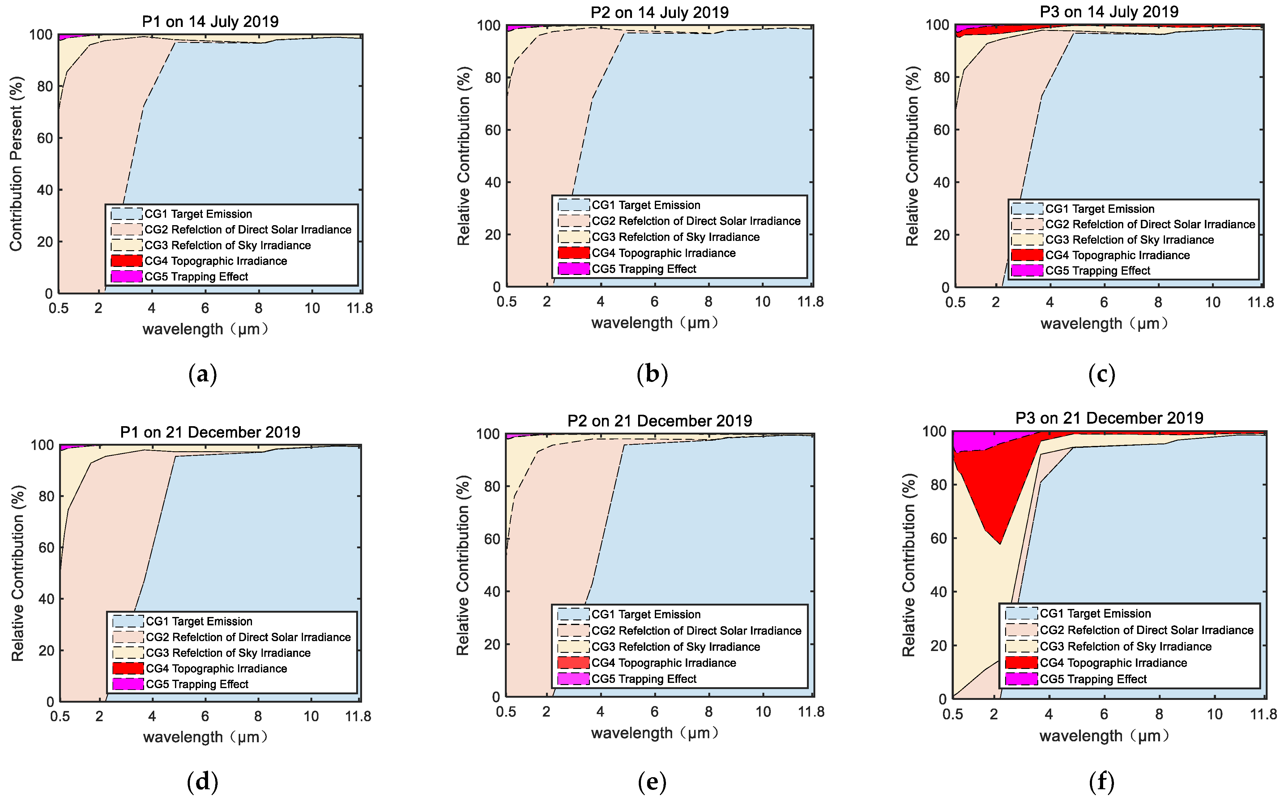
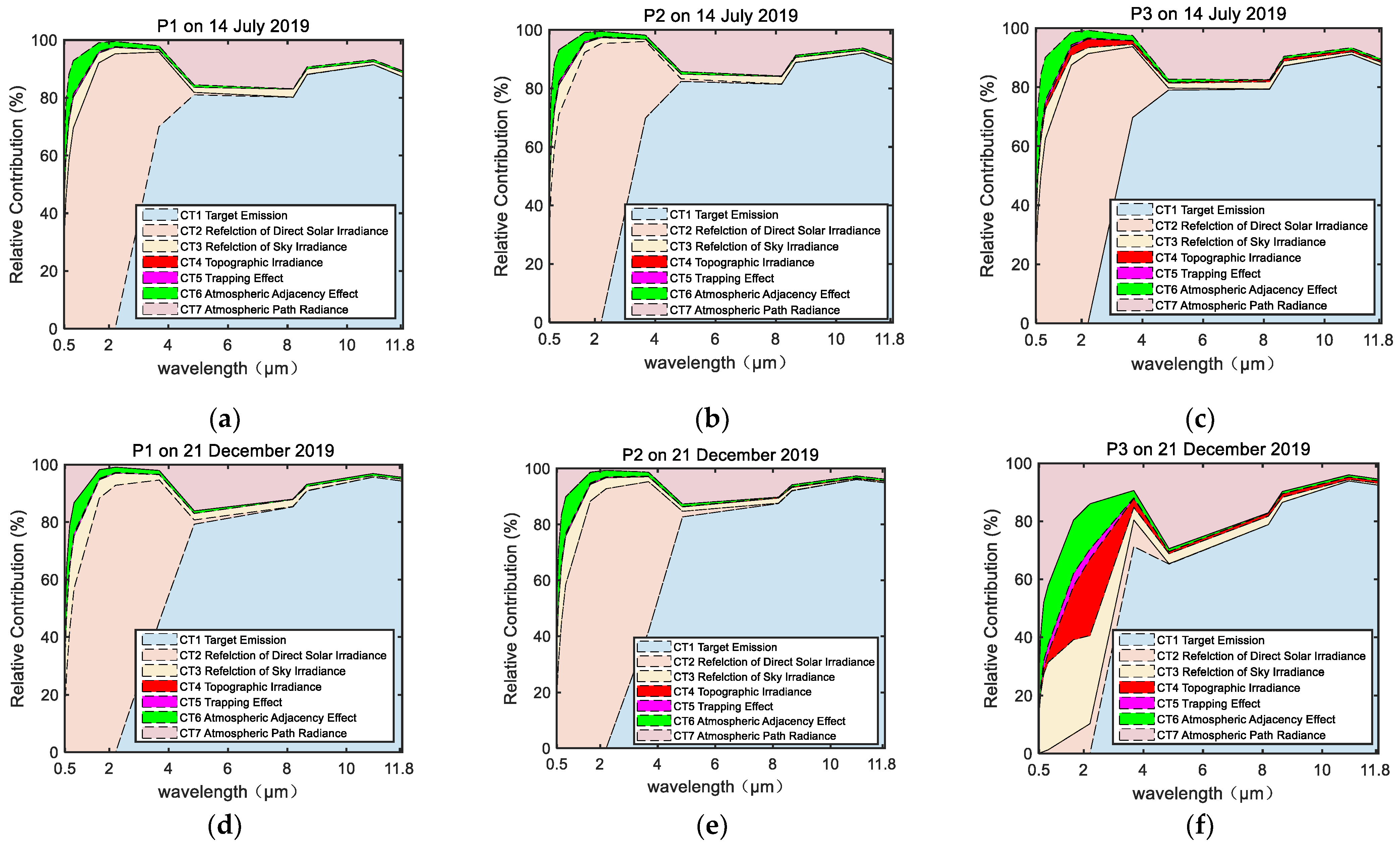
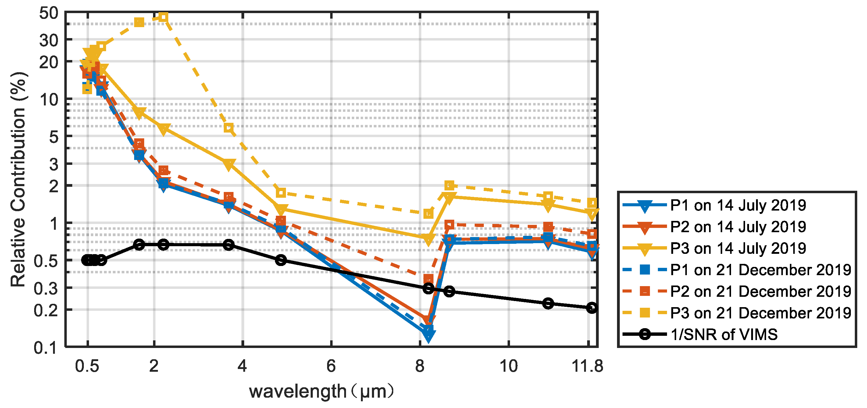
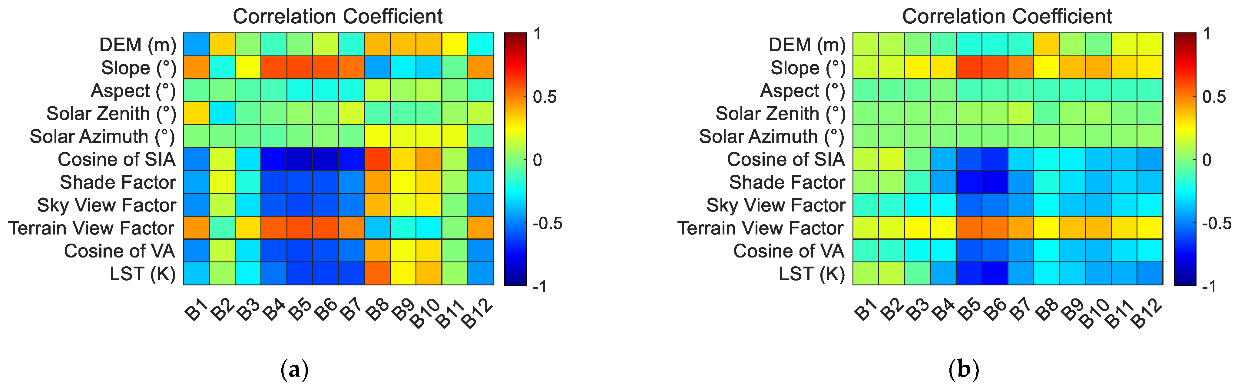
3.2. Evaluation of Atmospheric and Topographic Contributions

To simulate the spectral imaging TOA data of rugged land surfaces under a given observing geometry condition in the visible to thermal domain, the proposed simulation framework introduces seven different radiative components, as defined in (2). Removing the influence of the upward direct transmittance, the atmospheric adjacency effect, and the path radiance, the BOA radiance is made up of five different components, as shown in (9). Both the TOA and BOA radiance are influenced by the atmosphere and terrain coupling effects. Although their mechanisms are different, the seven TOA components and the five BOA components are all variates of atmospheric and topographic parameters. Recently, it is a common cognizance that topographic parameters influence radiation signals, especially the downward solar and sky irradiance. However, there is still a lack of quantitative evaluations of components caused by different atmosphere and terrain coupling mechanisms over the visible to thermal domain, to the best of our knowledge. For the evaluation of atmospheric and topographic contributions on radiance signals, the various components in TOA and BOA radiance are calculated and compared. The relative contribution of components in the BOA and TOA radiance at the three typical pixels mentioned in the last section are expressed as percentage and shown in Figure 12 and Figure 13, respectively. Thus, the component contribution order in the radiance signal of each pixel is clear.
Figure 12 illustrates that the reflection of the direct solar irradiance of the target is always the most significant component for the BOA radiance of the illuminated pixels (P1 and P2) in solar-reflected spectral region. The target emission is the most significant component in the spectral range from 4 μm to 12 μm, while the reflection of sky irradiance plays an important role through all the spectral bands, from visual to long-wave infrared (LWIR), especially for the shaded pixels, as shown in Figure 12f. The topographic irradiance effect is quite weak for the illuminated pixels, but remarkable for the shaded pixel. For the B6 of VIMS, with a central wavelength of 3.68 μm in the scene with the imaging date of 21 December 2019, the topographic irradiance contributes nearly 40% of the BOA radiance. Meanwhile, the trapping effect, which decreases when the wavelength increases, is more significant for the shaded pixel compared to illuminated pixels.
As shown in Figure 13, the atmospheric path radiance is the third significant component in TOA radiance, besides the target emission and the reflection of direct solar irradiance. The contribution of atmospheric path radiance is up to 76% of the condition at the first band of Figure 11f, which explains why the target recognition is harder in shadow areas. The adjacency effect on TOA radiance is the summation of the topographic irradiance, the trapping effect, and the atmospheric adjacency effect. Among the three adjacency effects, atmospheric adjacency effect is remarkable for all six of the conditions in Figure 13, while the topographic irradiance and the trapping effect contribute no more than 1% for the illuminated P1 and P2. As the contribution of topographic irradiance effect increases with the terrain shade, it constitutes 26% of the TOA radiance at B6 in Figure 13f. Although smaller contributions, caused by topographic irradiance and trapping effect, are observed in thermal domain than in the solar-reflected spectral domain, they are actually important for the shaded pixel P3, with a total contribution of 3% for B7.
The results in Figure 12 and Figure 13 illustrate that the adjacency effects caused by atmosphere and terrain have small, but unstable, contributions to the BOA and TOA radiance signals. Whether these adjacency effects could be ignored when using a specified imaging system becomes an important problem in the quantitative remote sensing. Taking the noise level assessment of VIMS as an example, the relative contribution of adjacency effects on TOA signal of different pixels are compared with the multiplicative inverse of SNR, as shown in Figure 14. The NEΔT values for B6 to B12 in Table 3 are converted to SNR at a signal level, defined by blackbody radiance with a temperature of 300 K. The multiplicative inverse of SNR is regarded as the relative radiation resolution of the imager. Figure 14 shows that the total relative contributions of the three adjacency effects on the TOA radiance are larger than the multiplicative inverse of SNR, for most spectral regions. The gaps between the relative contributions and the multiplicative inverse of SNR are obviously larger in the solar-reflected spectral domain than those in the thermal domain. The logarithmic axis method is used for the y-axis of this figure to display a more detailed contrast between plots in the thermal spectral domain. The spectral relative contributions of the three adjacency effects for the three typical pixels all have their smallest values at the band of B9, with a central wavelength of 8.19 μm. Only the contributions of the illuminated P1 and P2 pixels at B9 are smaller, or approximate to, the multiplicative inverse of SNR. In other words, only for the illuminated P1 and P2 pixels at B9 can the adjacency effects be ignored in the measured TOA signals. The relative contributions of the three adjacency effects are smaller than 5% over the thermal domain. It implies that these effects are not accurately measured when the restored TOA data has a relative measurement error of 5%, leading to uncertainty in remote sensing products.
As a preview of the errors on TOA brightness temperature products caused by ignoring the adjacency effects, the deviation of TOA brightness temperature (DTBT) of simulated images with, and without, the related three components are shown in Figure 15. Obviously, the influence of adjacency effects on DTBT is spectrally and spatially variable. The images show that the DTBT of the pixels in the valleys, with small sky view factors, is relatively higher than other pixels. In the flat and peak area, the DBT is mainly distributed in a range of 0.2 to 0.7 K for all four LWIR bands. For the valley pixels, the DTBT is larger than 1 K. The largest DTBT of 1.75 K appears at B10 on the day of 14 July 2019. Although the simulations are just taken under clear and sunny conditions, they also have referential values for people to recognize the uncertainty associated with adjacency effects over rugged areas in the visible to thermal spectral domain.

4. Discussion

Although the validation results demonstrate that the proposed atmosphere and terrain coupling simulation framework over visible to thermal domain could gather consistent and accurate simulations of onboard images, there are some issues that require attention when dealing with simulation and data processing tasks.

4.1. Topographic Error Accumulation

In the proposed simulation framework, all the TOA and BOA radiance components, and the simulated LST, are related to topographic features. The slope angle, aspect angle, cosine of SIA, shade factor, sky view factor, terrain view factor, the cosine of the viewing angle (VA, angle between the normal of pixel and the viewing direction of sensor), and the LST are collectively called as topographic variable factors here. Errors of all these topographic variable factors would accumulate in the simulated BOA and TOA spectral radiance. The terrain view factor in (25), with a value from 0 to 1, is introduced to depict the degree of adjacency illumination for discussion in this section.
V t 1 + cos α 2 V s k y
In order to identify the major topographic error sources, the correlation coefficients between the input topographic variable factors and the absolute values of relative deviation of the simulated and onboard images are shown in Figure 16. As the input atmospheric coefficients are spatially interpolated, according to the ground elevation, the DEM data is also discussed as a variable factor here. On the whole, the value of the topographic correlation of the summer scene is greater than that of the winter scene, which may be related to the different calibration accuracies of onboard data. However, Figure 16 provides a coherent view of the influence rank on overall accuracy of the proposed model over the visible to thermal domain. The influence rank, in descending order, is cosine of SIA, shade factor, slope, LST, cosine of VA, sky view factor, and terrain view factor, while the influence on simulation accuracy of the DEM and aspect angle are relatively nonlinear and indirectly transferred by other topographic variable factors. These key topographic variable factors are extracted from the DEM data. Slope and aspect angles are calculated directly from DEM, and they are mathematically correlative to each other. There would be error accumulation of topographic variable factors when radiative factors over rugged areas are calculated with these factors. Therefore, the quantitative description of errors and correlations of topographic variable factors is an interesting and important task in future studies to explain the BOA product uncertainties.

4.2. The Angle and Scale Effects

This study is built on the DEM data that describes the surface terrain and the 1D plane-parallel atmosphere assumption, which segments the atmospheric medium into horizontal layers. The validation experiments were taken from the simulation of the imaging data of a satellite observing the Earth along nadir direction. The GSD of DEM data used in the experimental study in this paper is 12.5 m. The whole atmospheric medium of 100 km in altitude was segmented into 28 layers, automatically following the segmentation rule of the auxiliary profile data. Currently, the validation experiments have not been conducted using airborne data, with GSD less than 10 m. In this circumstance, the angle and scale effects become a practical problem. A higher resolution of DEM data is required to solve the problems caused by composite slope effects and to gather accurate topographic parameters.
It is worth noting that the atmospheric PSF, as shown in (16), is a function of the viewing angle. For the nadir observation over flat surfaces, the atmospheric PSF is symmetrical with the highest value near the target pixel, because the aerosol scattering phase function peaks strongly in the forward direction. It is believed that the shape of atmospheric PSF is not important to the radiative results, as shown in previous literature such as [32]. Figure 17 presents the modeled atmospheric adjacency effect convolution function for typical pixel P3, under the nadir spaceborne viewing condition, and a tilt airborne viewing condition with view zenith angle of 20°. For the airborne condition, the integral calculation of atmospheric PSF was conducted with a refined vertical interval to 10 m, to decrease the extra error in numerical calculation. The shapes of these convolution functions are affected by local terrain and are not perfectly symmetrical. There is still a sharp peak near the target pixel, due to the nadir observation of spaceborne VIMS, as shown in Figure 17a. Nevertheless, for the airborne condition with tilt viewing directions and short transmission paths from ground to sensor, the geometric gravity center of the kernel function F moves away from the target location, as shown in Figure 17b. A single-peaked hypothesis is invalid for atmospheric PSF for the tilt airborne viewing conditions. This phenomenon is related to angle and scale effects, and would be serious for the edge pixels in the sensor’s field of view. Under the tilt viewing conditions, the ground-leaving radiance of more adjacency pixels would be scattered into the sensor’s IFOV. It is necessary to distinguish the local shape of atmospheric PSF varying with pixel locations.
However, these potential angle and scale effects on airborne conditions could be modeled using the proposed simulation framework, with appropriate input data. The proposed simulation framework would benefit future improvement of atmospheric correction methods over rugged land surfaces.

4.3. Challenges for Retrieval Applications

The forward simulation method is proven effective, as the results agree reasonably well with satellite observations statistically over a give rugged land scene. However, the proposed model could not be directly used for backward retrieval of LSE, reflectance, and LST. There are still some challenges needing attention before developing the atmospheric–topographic coupling correction methods.
(1) The measurement function of TOA radiance is an ill-posed function, with more independent variables than dependent variables. The backward retrieval needs to be simplified to the normal functions, or solved using iteration. Thus, parameterization of the initial LSE, reflectance, and LST with reliable prior knowledge, is the first challenge.
(2) The proposed model describes the 3D geometry of land surface using the public DEM data, with a rough GSD of 10 m to 100 m. Accurate descriptions of the terrain futures of pixels in the retrieval tasks requires the GSD of imaging data larger than the GSD of DEM data. Thus, the generation of fine and accurate geometry parameters is another challenge when dealing with complex 3D surfaces, such as the canopy and the buildings.
(3) The atmospheric–topographic coupling correction in the scene with clouds is also a large challenge. This study is conducted without the 3D effect of clouds, which are essential radiation sources for the land surface, as well as obstacles for both upward and downward radiation transfer. The 1D cloudy atmosphere influence on the atmospheric flux and the transmission could be modelled using the MODTRAN module in the proposed simulation framework. Moreover, the priori label layers of water clouds, cirrus clouds, and their cast shadow over the rugged surface are necessary in the retrieval tasks.

5. Conclusions

As the continuation of our previous work of the earth–atmosphere coupling model for solar-reflected hyperspectral systems [29], the model was improved and expanded to the entire spectral range, from visible to thermal. The atmosphere and terrain coupling simulation framework for high-resolution spectral imaging of heterogeneous land surfaces over visible to thermal domain was established in this study. The framework, in combination with the heat balance model of land surfaces, realized the simulation of high-resolution imaging signals including the LST, the BOA radiance, and the TOA radiance over rugged areas. There are two advantages of the simulation methodology: (I) it analytically models the topographic irradiance, trapping effect, and atmospheric adjacency effect with three spatial-spectral convolution kernels related to both atmospheric and terrain features, avoiding the commonly used assumption of independence between atmospheric and topographic adjacency effects; (II) it provides a novel method to establish layer atmosphere coefficients look-up tables based on multiple output files of MODTRAN, which benefits the imaging simulation for various viewing altitude and angles.
The simulation framework, and the produced data, could be used for the performance predictions of earth-observing systems, and serve to optimize spectral imaging missions. The accuracy of the TOA radiance simulation was validated using China’s Gaofen-5 VIMS data. The simulation experiment indicates that the proposed simulation framework is reliable. The spectral root mean square of relative deviations between simulated radiance and onboard radiance is less (larger) than 17% (3%) and 38% (6%) in the summer and winter scene, respectively. Some statistical evaluations of the atmospheric and topographic effects were also implemented. It indicates that the uncertainty associated with atmosphere and terrain coupling effects should be quantified under the whole cycle, from the concept design stage to the application stage, for a spectral imaging mission of earth.

Author Contributions

Conceptualization, X.Q., H.Z. and G.J.; investigation, X.Q.; methodology, X.Q. and G.J.; data curation, H.Z. and G.J.; supervision, H.Z.; validation, X.Q. and J.L.; writing—original draft, X.Q.; writing—review and editing, X.Q., G.J. and H.Z. All authors have read and agreed to the published version of the manuscript.

Funding

This research was funded by the National Key Research and Development Program of China, grant number 2016YFB0500502 and 2016YFB0500505.

Data Availability Statement

Not applicable.

Acknowledgments

The authors are grateful to the China Centre for Resources Satellite Data and Application and the Land Satellite Remote Sensing Application Center, MNR, China for providing the Gaofen-5 dataset for our investigations. The authors are grateful to the anonymous reviewers for their critical review, insightful comments, and valuable suggestions.

Conflicts of Interest

The authors declare no conflict of interest.

References

  1. Liang, S. Quantitative Remote Sensing of Land Surfaces; John Wiley & Sons, Inc.: Hoboken, NJ, USA, 2004; ISBN 0-471-28166-2. [Google Scholar]
  2. Kuenzer, C.; Dech, S. Thermal Infrared Remote Sensing; Springer: Dordrecht, The Netherlands, 2013; ISBN 978-94-007-6638-9. [Google Scholar]
  3. Fahlen, J.E.; Brodrick, P.G.; Thompson, D.R.; Herman, R.L.; Hulley, G.; Cawse-Nicholson, K.; Green, R.O.; Green, J.J.; Hook, S.J.; Miller, C.E. Joint VSWIR-TIR retrievals of earth’s surface and atmosphere. Remote Sens. Environ. 2021, 267, 112727. [Google Scholar] [CrossRef]
  4. Liu, Y.-N.; Zhang, J.; Sun, W.-W.; Jiao, L.-L.; Sun, D.-X.; Hu, X.-N.; Ye, X.; Li, Y.-D.; Liu, S.-F.; Cao, K.-Q.; et al. The Advanced Hyperspectral Imager: Aboard China’s GaoFen-5 Satellite. IEEE Geosci. Remote Sens. Mag. 2019, 7, 23–32. [Google Scholar] [CrossRef]
  5. Meng, X.; Cheng, J.; Zhou, S. Retrieving Land Surface Temperature from High Spatial Resolution Thermal Infrared Data of Chinese Gaofen-5. In Proceedings of the IEEE International Geoscience and Remote Sensing Symposium, Yokohama, Japan, 28 July–2 August 2019. [Google Scholar] [CrossRef]
  6. Zhao, Y.; Dai, L.; Bai, S.; Liu, J.; Peng, H.; Wang, H. Design and Implementation of Full-spectrum Spectral Imager System. Spacecr. Recovery Remote Sens. 2018, 39, 38–50. (In Chinese) [Google Scholar] [CrossRef]
  7. Schott, J.R. Remote Sensing: The Image Chain Approach; Oxford University Press: New York, NY, USA, 2007; ISBN 978-0-19-517817-3. [Google Scholar]
  8. Richter, R. Correction of atmospheric and topographic effects for high spatial resolution satellite imagery. Int. J. Remote Sens. 1997, 18, 1099–1111. [Google Scholar] [CrossRef]
  9. Shepherd, J.D.; Dymond, J.R. Correcting satellite imagery for the variance of reflectance and illumination with topography. Int. J. Remote Sens. 2003, 24, 3503–3514. [Google Scholar] [CrossRef]
  10. Santini, F.; Palombo, A. Physically Based Approach for Combined Atmospheric and Topographic Corrections. Remote Sens. 2019, 11, 1218. [Google Scholar] [CrossRef] [Green Version]
  11. Yan, G.; Wang, T.; Jiao, Z.; Mu, X.; Zhao, J.; Chen, L. Topographic radiation modeling and spatial scaling of clear-sky land surface longwave radiation over rugged terrain. Remote Sens. Environ. 2016, 172, 15–27. [Google Scholar] [CrossRef]
  12. Zheng, X.; Li, Z.-L.; Zhang, X.; Shang, G. Quantification of the Adjacency Effect on Measurements in the Thermal Infrared Region. IEEE Trans. Geosci. Remote Sens. 2019, 57, 9674–9687. [Google Scholar] [CrossRef]
  13. Yan, G.; Jiao, Z.-H.; Wang, T.; Mu, X. Modeling surface longwave radiation over high-relief terrain. Remote Sens. Environ. 2020, 237, 111556. [Google Scholar] [CrossRef]
  14. Duan, S.-B.; Li, Z.-L.; Gao, C.; Zhao, W.; Wu, H.; Qian, Y.; Leng, P.; Gao, M. Influence of adjacency effect on high-spatial-resolution thermal infrared imagery: Implication for radiative transfer simulation and land surface temperature retrieval. Remote Sens. Environ. 2020, 245, 111852. [Google Scholar] [CrossRef]
  15. Zhu, X.; Duan, S.-B.; Li, Z.-L.; Zhao, W.; Wu, H.; Leng, P.; Gao, M.; Zhou, X. Retrieval of Land Surface Temperature with Topographic Effect Correction from Landsat 8 Thermal Infrared Data in Mountainous Areas. IEEE Trans. Geosci. Remote Sens. 2021, 59, 6674–6687. [Google Scholar] [CrossRef]
  16. Berk, A.; Anderson, G.P.; Acharya, P.K. MODTRAN 5.3.2 User’s Manual; Spectral Sciences, Inc.: Burlington, MA, USA; Air Force Research Laboratory, Hanscom AFB: Albuquerque, NM, USA, 2013. [Google Scholar]
  17. Vermote, E.F.; Tanré, D.; Deuze, J.L.; Herman, M.; Morcette, J.J. Second Simulation of the Satellite Signal Second Simulation of the Satellite Signal in the Solar Spectrum, 6S: An Overview. IEEE Trans. Geosci. Remote Sens. 1997, 35, 675–686. [Google Scholar] [CrossRef] [Green Version]
  18. Clough, S.A.; Iacono, M.J.; Moncet, J.-L. Line-by-line calculations of atmospheric fluxes and cooling rates: Application to water vapor. J. Geophys. Res. 1992, 97, 15761–15785. [Google Scholar] [CrossRef]
  19. Clough, S.; Shephard, M.; Mlawer, E.; Delamere, J.; Iacono, M.; Cady-Pereira, K.; Boukabara, S.A.; Brown, P. Atmospheric radiative transfer modeling: A summary of the AER codes. J. Quant. Spectrosc. Radiat. Transf. 2005, 91, 233–244. [Google Scholar] [CrossRef]
  20. Schott, J.R.; Brown, S.D.; Raqueno, R.V.; Gross, H.N.; Robinson, G. Advanced synthetic image generation models and their application to multi/hyperspectral algorithm development. In Proceedings of the 27th AIPR Workshop: Advances in Computer-Assisted Recognition, Washington, DC, USA, 14 October 1998; Mericsko, R.J., Ed.; pp. 211–220. [Google Scholar]
  21. Goodenough, A.A.; Brown, S.D. DIRSIG5: Next-Generation Remote Sensing Data and Image Simulation Framework. IEEE J. Sel. Top. Appl. Earth Obs. Remote Sens. 2017, 10, 4818–4833. [Google Scholar] [CrossRef]
  22. Sundberg, R.L.; Berk, A.; Richtsmeier, S.; Adler-Golden, S.M.; Haren, R. Hyperspectral scene simulation from the visible through the LWIR. Proc. SPIE 2004, 5234, 252–261. [Google Scholar] [CrossRef]
  23. Grau, E.; Gastellu-Etchegorry, J.-P. Radiative transfer modeling in the Earth–Atmosphere system with DART model. Remote Sens. Environ. 2013, 139, 149–170. [Google Scholar] [CrossRef]
  24. Wu, S.; Wen, J.; You, D.; Hao, D.; Lin, X.; Xiao, Q.; Liu, Q.; Gastellu-Etchegorry, J.-P. Characterization of Remote Sensing Albedo Over Sloped Surfaces Based on DART Simulations and In Situ Observations. J. Geophys. Res. Atmos. 2018, 123, 8599–8622. [Google Scholar] [CrossRef]
  25. Spurr, R.; Kurosu, T.P.; Chance, K.V. A linearized discrete ordinate radiative transfer model for atmospheric remote-sensing retrieval. J. Quant. Spectrosc. Radiat. Transf. 2001, 68, 689–735. [Google Scholar] [CrossRef]
  26. Borel, C.C.; Gerstl, S.A.W.; Powers, B.J. The radiosity method in optical remote sensing of structured 3-D surfaces. Remote Sens. Environ. 1991, 36, 13–44. [Google Scholar] [CrossRef]
  27. Borel, C.C.; Gerstl, S.A.W. Simulation of partially obscured scenes using the radiosity method. In Proceedings of the Orlando ‘91, Characterization, Propagation, and Simulation of Sources and Backgrounds, Orlando, FL, USA, 1 April 1991; Watkins, W.R., Clement, D., Eds.; pp. 271–277. [Google Scholar]
  28. Borel, C.C.; Gerstl, S.A.W. Adjacency-blurring-effect of scenes modeled by the radiosity method. In Proceedings of the SPIE Aerospace Sensing, Atmospheric Propagation and Remote Sensing, Orlando, FL, USA, 20 April 1992; Kohnle, A., Miller, W.B., Eds.; pp. 620–624. [Google Scholar]
  29. Zhao, H.; Jia, G.; Li, N. Transformation from Hyperspectral Radiance Data to Data of Other Sensors Based on Spectral Superresolution. IEEE Trans. Geosci. Remote Sens. 2010, 48, 3903–3912. [Google Scholar] [CrossRef]
  30. Florio, C.J.; Cota, S.A.; Gaffney, S.K. Predicting top-of-atmosphere radiance for arbitrary viewing geometries from the visible to thermal infrared: Generalization to arbitrary average scene temperatures. In Proceedings of the SPIE Optical Engineering + Applications, San Diego, CA, USA, 1–5 August 2010. [Google Scholar] [CrossRef]
  31. Liu, Y.; Zhang, W.; Zhang, B. Top-of-Atmosphere Image Simulation in the 4.3-μm Mid-infrared Absorption Bands. IEEE Trans. Geosci. Remote Sens. 2016, 54, 452–456. [Google Scholar] [CrossRef]
  32. Verhoef, W.; Bach, H. Simulation of hyperspectral and directional radiance images using coupled biophysical and atmospheric radiative transfer models. Remote Sens. Environ. 2003, 87, 23–41. [Google Scholar] [CrossRef]
  33. Verhoef, W.; Bach, H. Simulation of Sentinel-3 images by four-stream surface–atmosphere radiative transfer modeling in the optical and thermal domains. Remote Sens. Environ. 2012, 120, 197–207. [Google Scholar] [CrossRef]
  34. Mousivand, A.; Verhoef, W.; Menenti, M.; Gorte, B. Modeling Top of Atmosphere Radiance over Heterogeneous Non-Lambertian Rugged Terrain. Remote Sens. 2015, 7, 8019–8044. [Google Scholar] [CrossRef] [Green Version]
  35. Shi, H.; Xiao, Z.; Wen, J.; Wu, S. An Optical–Thermal Surface–Atmosphere Radiative Transfer Model Coupling Framework With Topographic Effects. IEEE Trans. Geosci. Remote Sensing 2022, 60, 1–12. [Google Scholar] [CrossRef]
  36. Zhao, H.; Jiang, C.; Jia, G.; Tao, D. Simulation of hyperspectral radiance images with quantification of adjacency effects over rugged scenes. Meas. Sci. Technol. 2013, 24, 5405. [Google Scholar] [CrossRef]
  37. Goel, N.S.; Rozehnal, I.; Thompson, R.L. A computer graphics based model for scattering from objects of arbitrary shapes in the optical region. Remote Sens. Environ. 1991, 36, 73–104. [Google Scholar] [CrossRef]
  38. Miesch, C.; Briottet, X.; Kerr, Y.H. Phenomenological Analysis of Simulated Signals Observed Over Shaded Areas in an Urban Scene. IEEE Trans. Geosci. Remote Sens. 2004, 42, 434–442. [Google Scholar] [CrossRef]
  39. Miesch, C.; Briottet, X.; Kerr, Y.H.; Cabot, F. Monte Carlo approach for solving the radiative transfer equation over mountainous and heterogeneous areas. Appl. Opt. 1999, 38, 7419–7430. [Google Scholar] [CrossRef]
  40. Sanders, L.C.; Schott, J.R.; Raqueño, R. A VNIR/SWIR atmospheric correction algorithm for hyperspectral imagery with adjacency effect. Remote Sens. Environ. 2001, 78, 252–263. [Google Scholar] [CrossRef]
  41. Diner, D.; Martonchik, J. Influence of Aerosol Scattering on Atmospheric Blurring of Surface Features. IEEE Trans. Geosci. Remote Sens. 1985, GE-23, 618–624. [Google Scholar] [CrossRef]
  42. Santer, R.; Schmechtig, C. Adjacency effects on water surfaces: Primary scattering approximation and sensitivity study. Appl. Opt. 2000, 39, 361–375. [Google Scholar] [CrossRef] [PubMed]
  43. Liou, K.-N. An introduction to Atmospheric Radiation, 2nd ed.; Academic Press: Amsterdam, The Netherlands; Boston, MA, USA, 2002; ISBN 0080491677. [Google Scholar]
  44. Guanter, L.; Richter, R.; Kaufmann, H. On the application of the MODTRAN4 atmospheric radiative transfer code to optical remote sensing. Int. J. Remote Sens. 2009, 30, 1407–1424. [Google Scholar] [CrossRef]
  45. Zhou, Q.; Liu, X. Analysis of errors of derived slope and aspect related to DEM data properties. Comput. Geosci. 2004, 30, 369–378. [Google Scholar] [CrossRef]
  46. Wang, J.; Robinson, G.J.; White, K. A Fast Solution to Local Viewshed Computation Using Grid-Based Digital Elevation Models. Photogramm. Eng. Remote Sens. 1996, 62, 1157–1164. [Google Scholar] [CrossRef]
  47. Dozier, J.; Frew, J. Rapid calculation of terrain parameters for radiation modeling from digital elevation data. IEEE Trans. Geosci. Remote Sens. 1990, 28, 963–969. [Google Scholar] [CrossRef]
  48. Karra, K.; Kontgis, C.; Statman-Weil, Z.; Mazzariello, J.C.; Mathis, M.; Brumby, S.P. Global land use / land cover with Sentinel 2 and deep learning. In Proceedings of the 2021 IEEE International Geoscience and Remote Sensing Symposium IGARSS, Brussels, Belgium, 11–16 July 2021. [Google Scholar] [CrossRef]
  49. ASF Data Search. Available online: https://search.asf.alaska.edu (accessed on 20 February 2022).
  50. Qiu, X.; Jia, G.; Zhao, H.; Zhang, C. Antinoise Estimation of Temperature and Emissivity for FTIR Spectrometer Data Using Spectral Polishing Filters: Design and Comparison. IEEE Trans. Geosci. Remote Sens. 2021, 59, 3292–3308. [Google Scholar] [CrossRef]
  51. Salisbury, J.W.; Wald, A.; D’Aria, D.M. Thermal-infrared remote sensing and Kirchhoff’s law: 1 Laboratory measurements. J. Geophys. Res. Earth Surf. 1994, 99, 11897–11911. [Google Scholar] [CrossRef]
  52. Baldridge, A.M.; Hook, S.J.; Grove, C.I.; Rivera, G. The ASTER spectral library version 2. Remote Sens. Environ. 2009, 113, 711–715. [Google Scholar] [CrossRef]
  53. Copernicus Climate Data Store | Copernicus Climate Data Store. Available online: https://cds.climate.copernicus.eu (accessed on 20 February 2022).
  54. EUMETSAT NWP SAF IR_SRF of GF5 VIMS. Available online: https://nwp-saf.eumetsat.int/downloads/rtcoef_rttov13/ir_srf/rtcoef_gf5_1_vims_srf.html (accessed on 20 February 2022).
  55. Tao, D.; Jia, G.; Yuan, Y.; Zhao, H. A digital sensor simulator of the pushbroom Offner hyperspectral imaging spectrometer. Sensors 2014, 14, 23822–23842. [Google Scholar] [CrossRef] [PubMed] [Green Version]
Figure 1. Schematic of the sun–surface–atmosphere–sensor system radiation signal composition. Seven components of at-sensor radiance are numbered sequentially, and shown as 1 to 7.
Remotesensing 14 02043 g001
Figure 2. Topographic illuminating geometry.
Remotesensing 14 02043 g002
Figure 3. Trapping effect between atmosphere and the rugged land surface. (a) is the successive reflection of land surface thermal emissions; (b) is the successive reflection of the solar and sky irradiance; (c) is the successive reflection of the emission irradiance from adjacent pixels; and (d) is the successive reflection of the adjacent irradiance caused by solar and sky irradiance.
Remotesensing 14 02043 g003
Figure 4. Atmospheric adjacency effect over the rugged land surface.
Remotesensing 14 02043 g004
Figure 5. The flow of simulation and evaluation.
Remotesensing 14 02043 g005
Figure 6. Auxiliary data for simulation. (a) is ERA5 world cover data; (b) is ALOS DEM data; (c) and (d) are reflectance spectra for scene generation of VIMS B1 to B6 bands and B7 to B12, respectively; (e) is the relative humidity profile observed by radiosonde; and (f) is temperature profile from ERA5 and the radiosonde observation site.
Remotesensing 14 02043 g006
Figure 7. Simulated land surface temperature and shade factor. (a,b) represent the simulated temperature under the flat surface assumption for the summer and winter scene, respectively; (c,d) represent the simulated temperature under the rugged surface assumption for the summer and winter scene, respectively; and (e,f) are the product matrixes of the shade factor and the cosine of SIA for the summer and winter scene, respectively.
Remotesensing 14 02043 g007
Figure 8. True color image comparison of the simulated TOA radiance. (a,c) are the simulated image under the flat surface assumption of the summer and winter scene, respectively; (b,d) are the images under the rugged surface assumption.
Remotesensing 14 02043 g008
Figure 9. The simulated and onboard restored TOA radiance. (a,b) are the B1 to B6 bands and B7 to B12 bands of VIMS TOA radiance with imaging date of 14 July 2019, while (c,d) are the imaging data of 21 December 2019, correspondingly. The radiance unit is “W/m2/sr/μm”.
Remotesensing 14 02043 g009
Figure 10. TOA spectra comparison of representative areas with different land covers. (a,c,d) are the TOA spectra of ROIs with land cover of Cropland, Water, and Desert, respectively; (b) is the TOA spectra for a typical pixel with land cover of Road in the urban areas.
Remotesensing 14 02043 g010
Figure 11. TOA spectra comparison of representative pixels with different degrees of surface relief.
Remotesensing 14 02043 g011
Figure 12. Atmospheric and topographic contributions on the BOA radiance. (ac) are the contribution plots of three typical pixels marked as P1, P2 and P3 in the scene imaging on 14 July 2019, respectively; (df) are contribution plots of 21 December 2019, respectively.
Remotesensing 14 02043 g012
Figure 13. Atmospheric and topographic contributions on the TOA radiance. (ac) are the contribution plots of three typical pixels marked as P1, P2 and P3 in the scene imaging on 14 July 2019, respectively; (df) are contribution plots of 21 December 2019, respectively.
Remotesensing 14 02043 g013
Figure 14. Overall contributions of atmospheric and topographic adjacency effects on TOA radiance.
Remotesensing 14 02043 g014
Figure 15. The deviation of TOA brightness temperature caused by atmospheric and topographic adjacency effects. (ad) are the deviation of TOA brightness temperature images of B9 to B12 bands on 14 July 2019, respectively; (eh) are the deviation of TOA brightness temperature images of B9 to B12 bands on 21 December 2019, respectively.
Remotesensing 14 02043 g015
Figure 16. Correlation coefficient between topographic variable factors and absolute values of relative deviation between simulated and onboard images. (a) is for the scene of 14 July 2019 and (b) is for the scene of 21 December 2019.
Remotesensing 14 02043 g016
Figure 17. The atmospheric adjacency effect convolution function for typical pixel P3. The x-axis and y-axis are spatial distance away from the target pixel. (a) is under a nadir viewing condition by spaceborne imager; (b) is under a tilt viewing condition by airborne imager.
Remotesensing 14 02043 g017
Table 1. Terrain parameters generation.
Terrain ParameterSymbolCalculation Method
Slope angle α α = arctan ( f x 2 + f y 2 )
where the inverse square distance weighted spatial interpolation of DEM [45], was used to calculate, f x and f y along a west–east and south–north direction, respectively.
Aspect angle β β = 270 + arctan ( f y / f x ) 90 × f x / | f x |
Cosine of SIA cos ( θ i ) cos θ i = cos α cos θ s + sin α sin θ s cos ( β ϕ s )
Shade factorSFShade factor was calculated using the depth buffer method.
Sky view Factor V s k y V s k y 1 2 π 0 2 π [ cos α sin 2 h ϕ + sin α cos ( ϕ β ) ( h ϕ sin h ϕ cos h ϕ ) ] d ϕ
where h ϕ is defined as the angle between the zenith and the horizon surface at a given orientation direction ϕ [46,47].
Table 2. Atmospheric parameters generation.
Atmospheric CoefficientsSymbolCalculation Using the MODTRAN Output Data
Hemispherical scattering albedo of BOA 1 S S = int e r p ( D E M , S P H E R I C A L   A L B E D O   F R O M   G N D )
Direct transmittance 1 τ d i r τ d i r = int e r p ( D E M , O B S _ G N D   D I R E C T   T R A N S M )
Diffuse transmittance 1 τ d i f τ d i f = int e r p ( D E M , O B S _ G N D   D I F   T R A N S M )
Path radiance 2 L a L a = int e r p ( D E M , P T H _ T H R M L + S O L _ S C A T )
Direct solar irradiance 3 E i n , d i r E i n , d i r = int e r p ( D E M , F L U X D I R E C T _ S O L A R )
Diffused solar irradiance 3 E i n , d i f E i n , d i f = int e r p ( D E M , F L U X D O W N _ D I F F ( S o l a r ) )
Diffused thermal irradiance from sky 3 E i n , t h e r m E i n , t h e r m = int e r p ( D E M , F L U X D O W N _ D I F F ( T h e r m a l ) )
Extinction coefficient of layers 3 k k i = 1 z l a y e r , i ln ( F L U X D I R E C T _ S O L A R , i + F L U X D O W N _ D I F F , i F L U X D I R E C T _ S O L A R , i + 1 + F L U X D O W N _ D I F F , i + 1 )
where z l a y e r , i is the height interval of the ith layer.
Scattering coefficient of layers 4 ς ς a e r o , i = 1 z l a y e r , i j = 1 4 S C A T _ D E P A E R O j , i
ς m o l e , i = S C A T _ D E P R A Y L E I G H , i / z l a y e r , i
1 The coefficient is derived from information in the “acd” file. 2 The coefficient is derived from information in the “tp7” file. 3 The coefficient is calculated using information in the “flx” file. 4 The coefficient is calculated using information in the “fort69” file.
Table 3. Imaging information and instrument performance parameters of Gaofen-5 VIMS.
Scene NumberScene 1Scene 2
Imaging time (UTC)14 July 2019 6:38:4521 December 2019 6:36:20
Average solar zenith angle (°)21.4064.90
Solar azimuth (°)214.43194.44
View zenith angle (°)0.160.17
View azimuth angle (°)131.04129.94
Quick view(true color) Remotesensing 14 02043 i001 Remotesensing 14 02043 i002
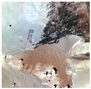
Instrument performance parameters of VIMS
Band numberB1-B4B5-B6B7-B8B9-B12
Band rangeB1: 0.44–0.51 μm
B2: 0.51–0.58 μm
B3: 0.62–0.68 μm
B4: 0.76–0.87 μm
B5: 1.54–1.70 μm
B6: 2.06–2.35 μm
B7: 3.45–3.90 μm
B8: 4.76–4.96 μm
B9: 8.05–8.45 μm
B10: 8.57–8.93 μm
B11: 10.5–11.3 μm
B12: 11.4–12.5 μm
GSD (m)20204040
SNR200150--
NEΔT (K)--0.15K@300K0.15K@300K
MTF0.20.30.150.15
Table 4. Root mean square of relative deviation between simulated and onboard TOA radiance.
Band (Central Wavelength)14 July 201921 December 2019
B1 (0.49 μm)6.94 %11.73%
B2 (0.56 μm)9.93%19.55%
B3 (0.66 μm)7.89%20.99 %
B4 (0.81 μm)15.64%30.44 %
B5 (1.66 μm)11.64%37.15%
B6 (2.21 μm)15.15%37.31%
B7 (3.68 μm)9.58%22.28%
B8 (4.86 μm)16.49%16.61%
B9 (8.19 μm)5.57%7.27%
B10 (8.66 μm)6.69%6.78%
B11 (10.89 μm)7.72 %10.19%
B12 (11.88 μm)3.35%11.47%
Table 5. Relative deviation between the restored TOA radiance of VIMS and AHSI.
Typical PointImaging TimeRelative Deviation
B1B2B3B4B5B6
P114 July 2019−3.00%0.15%2.08%−5.97%18.37%17.57%
21 December 2019−2.49%−1.27%0.46%−6.30%20.92%21.36%
P214 July 2019−4.17%−2.78%−2.70%−5.19%11.90%12.23%
21 December 2019−1.99%0.24%2.30%0.22%35.85%31.89%
P314 July 2019−2.95%−0.52%1.66%−3.07%−3.34%4.75%
21 December 2019−4.50%−9.31%−12.46%−15.90%−150.20%−156.96%
Publisher’s Note: MDPI stays neutral with regard to jurisdictional claims in published maps and institutional affiliations.

