A General Spline-Based Method for Centerline Extraction from Different Segmented Road Maps in Remote Sensing Imagery

Abstract

Road centerline extraction is the foundation for integrating the segmented road map from a remote sensing image into a geographic information system (GIS) database. Considering that existing approaches tend to have a decline in performance for centerline and junction extraction when segmented road structures are irregular, this paper proposes a novel method which models the road network as a sequence of connected spline curves. Based on this motivation, the ratio of cross operators is firstly proposed to detect direction and width features of roads. Then, road pixels are divided into different clusters by local features using three perceptual grouping principles (i.e., direction grouping, proximity grouping, and continuity grouping). After applying a polynomial curve fitting on each cluster using pixel coordinates as observation data, the internal control points are determined according to the adjacency relation between clusters. Finally, road centerlines are generated based on spline fitting with constraints. We test our approach on segmented road maps which were obtained previously by machine recognition, or manual extraction from real optical (WorldView-2) and synthetic aperture radar (TerraSAR-X, Radarsat-2) images. Depending on the accuracy of the input segmented road maps, experimental results from our test data show that both the completeness and correctness of extracted centerlines are over 84% and 68% for optical and radar images, respectively. Furthermore, experiments also demonstrate the advantages of our proposed method, in contrast to existing methods for gaining smooth centerlines and precise junctions.

1. Introduction

Road databases play an essential role in modern transportation systems. With the development of remote sensing technology, remote sensing images have become one of the main sources of road information acquisition. Starting from a remote sensing image, road centerline extraction is one of the key technologies for practical applications, such as road data updates in geographic information systems (GISs). Although manual marking of road centerline is more accurate, it is a time-consuming and labor-intensive task; therefore, automatic or semi-automatic road centerline extraction from remote sensing data has been a significant research activity during past decades [1]. Nevertheless, because of the data noise, the diversity of road types and complex backgrounds surrounding the road, extracting complete and correct centerlines automatically is still challenging.

Until now, a variety of road centerline extraction methods have been proposed from different viewpoints. In general, there are two kinds of methods for road centerline extraction. One is tracking road centerlines directly from remote sensing images. For example, Zhou et al. [2] introduced a road tracking system based on human–computer interactions and Bayesian filtering. Cheng et al. [3] proposed using a parallel particle filter to track road centerlines. Dal Poz et al. [4] presented a methodology which extracts road seeds first with local road property and then links them among road seeds. The other is the most widely utilized, which segments road areas from images first, and then detects the final centerlines. Based on this framework, road centerlines are generally extracted using one of the following: (1) traditional thinning algorithms, such as morphology thinning [1,5,6]; (2) tensor voting [7,8,9]; (3) non-maximum suppression (NMS) [8,10,11]; and (4) convolutional neural networks (CNN) [12]. Moreover, Negri et al. [13] realized the road skeleton extraction using an incremental tracking approach from SAR images. Among these methods, traditional thinning algorithms have a quick response, but may result in small spurs or loops instead of neat curves when segmented roads have no regular shapes. For tensor voting, it is time consuming, and an extra connection step to fill gaps is needed. NMS algorithms retain local maximum positions as centerlines, as it largely depends on the computation of the centerline response map. CNN is a highly effective supervision method which requires a large amount of sample data. In practical applications, time cost is often a considerable factor. Moreover, the accuracy of road junctions is of high importance when constructing road network topologies; therefore, as for road centerline extraction from remote sensing images, there is room for further research.

Regarding the data sources considered, there are mainly three types of remote sensing data used for road centerline extraction, which are optical images, synthetic aperture radar (SAR) images, and light detection and ranging (LiDAR) data. Optical imagery is most widely used because of its advantages concerning high spatial resolution and high road discrimination, but its acquisition is easily affected by cloud and rain. As for SAR images, although they are available in all weather conditions and around the clock, the difficulty for such imagery lies in solving multiplicative noise, and reducing the confusion of roads, water bodies, and shadows [14]. LiDAR is a technology that can provide three-dimensional information, and also can weaken the influence of tree obscuration on road extraction; although, for such images, the non-road impervious surfaces can easily be misidentified as roads [15]. Although the segmented road maps obtained from different sources or different segmentation methods may show different features, this paper proposes a general approach for road centerline extraction from different segmented road maps in optical (WorldView-2) and SAR (TerraSAR-X, Radarsat-2) images.

Here, we develop a road centerline extraction method from the segmented road map based on perceptual grouping and spline fitting. There are three main contributions that are worth mentioning. Firstly, a novel ratio of cross (RoC) operator is proposed to extract direction and the width feature of roads. Secondly, perceptual grouping principles and their specific implementations are presented to cluster road pixels. Thirdly, spline fitting with constraints by control points is innovatively proposed to construct the final road centerline network.

The rest of this paper is organized as follows. The proposed method with a general scheme is introduced in detail in Section 2 and Section 3. The experimental validation, parameter settings, and comparison results are shown in Section 4. Section 5 shows the parameter sensitivity evaluation results. The conclusions and suggested applications are given in Section 6.

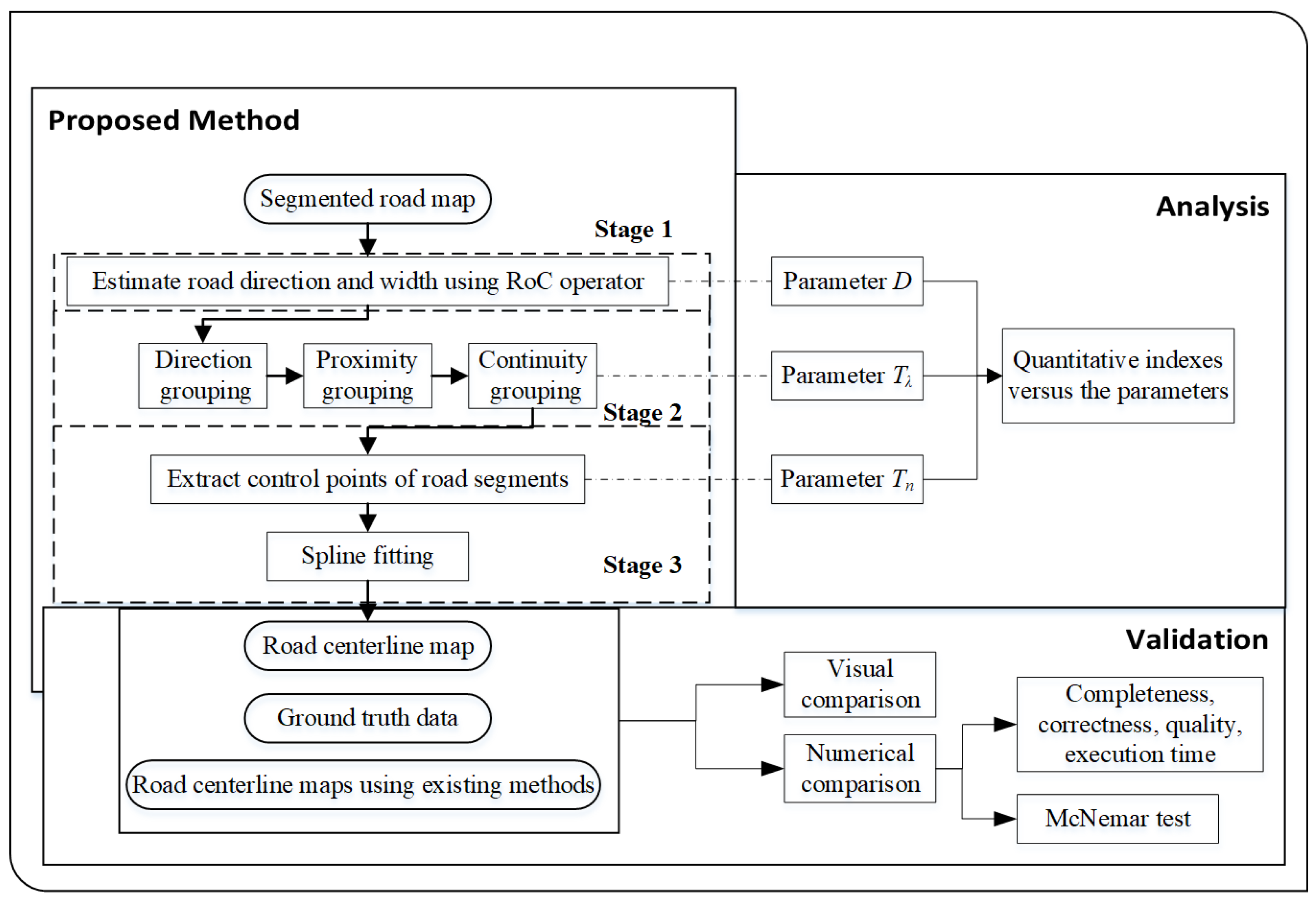
2. General Scheme of the Method

The general scheme of proposed approach is summarized in Figure 1, together with the diagrammatic sketches of the validation and analysis processes. Starting with a segmentation result of road pixels from the remote sensing images, a three-stage procedure for road centerline extraction is presented. The segmented road binary map contains information of road shape, edges, and widths. We aim to detect the road centerline automatically from the road binary map obtained by different methods. In this paper, the road segmentation method in [16] is applied for obtaining optical images, the method in [17] is used to obtain SAR images, and the hand marking method is also applied. Then, the presented centerline extraction procedure is described by means of three stages, which are (1) using a ratio of cross (RoC) operation to derive road orientation and width; (2) clustering road pixels based on three perceptual grouping principles; and (3) extracting control points and generating the road centerline map by spline fitting. It can also be observed that the proposed method is validated visually and numerically by comparing extraction results with ground truth data. Notably, the McNemar test is applied to measure the differences of extraction results using different approaches. For the analysis, the effects of three key parameters on the accuracy of the extraction results are discussed in detail.

3. Methodology

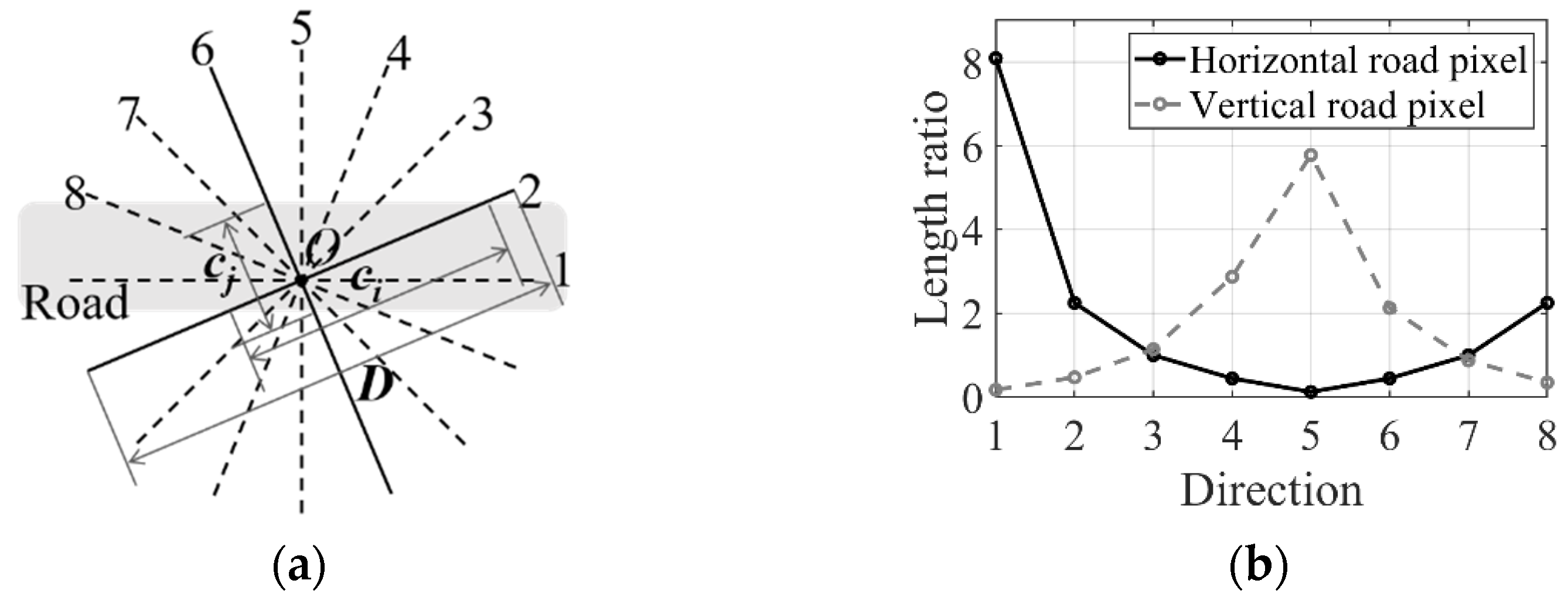
3.1. Ratio of Cross Detector for Feature Extraction

In this section, a novel detector named ratio of cross (RoC) is proposed for extracting features of road direction and width. In high-resolution remote sensing images, roads usually appear as an elongated area with a specific width. Based on these characteristics, RoC is designed for computing the length ratios in a circular window at the road pixel (See Figure 2a). Given the diameter $D$ of window and the number $N$ of the direction division, the direction $v$ of the current road pixel can be expressed as

$$v=\arg \underset{i}{\max }\left\{\frac{c_i}{c_j}\right|i\perp j;i,j=1,2,\mathrm{\dots },N\}.$$

(1)

where $c_i$ and $c_j$ denote the length of the line covered by road pixels at the direction $i$ and $j$ which are perpendicular to each other. Then, the width $w$ of the current center pixel is estimated by $w=c_u$ where $u\perp v$. In the case of $N=8$ shown in Figure 2a, it can be inferred that $c_1/c_8$ is the maximum value of $c_i/c_j$ and thus direction 1 will be the detected direction for road pixel $O$. In the implementation, the value of $c_i$ can be estimated using image convolution with a linear structuring element towards a specific direction. Figure 2b presents the length ratios at a different direction for two test road pixels which belong to horizontal and vertical road segments, respectively. It has been proven that the maximum length ratio is able to highlight the orientation of sampled road pixels. Furthermore, Figure 3 shows an example of the application of the RoC detector. The colored areas in (a), (b), and (c) of Figure 3 correspond to road regions. Different directions and width values derived from RoC detectors are labelled with different colors. Considering that a pixel belonging to a direction $i$ is likely to have neighboring pixels belonging to the same direction, a Markov random fields (MRF) [18] framework is applied to the original direction map for de-noising (i.e., obtaining a “cleaner” road direction map). Figure 3b presents the de-noising result which uses Figure 3a as an initialization.

3.2. Object-Based Perceptual Grouping for Clustering

The concept of perceptual grouping is proposed based on the phenomenon that human observers often show a capability to perceptually put parts together into a whole [19]. In this paper, road pixels with a similar direction and width are expected to be grouped into clusters, which will be the base unit for spline fitting to construct the final road centerlines. To this end, three perceptual grouping rules are proposed in detail in the following sections.

3.2.1. Direction Grouping

According to the detected orientation feature on the road direction map, it is easy to notice that road regions have been separated piece by piece. When describing roads, from pixels to segments, the connected–component (CC) labeling [20] method is firstly applied on a road map at each direction feature. In other words, connected road pixels with the same direction feature are combined into one cluster. We call this step direction grouping. For illustrative purposes, let us denote by $S=\left\{s\right\}$ the set of clusters where $s$ is a set of pixel points in CC. According to the adjacency relation, we define a set of neighbors for each cluster and denote this by $\delta (s)$. That is, $\delta (s)=\left\{t\right|t\in S,t\leftrightarrow s\}$ where $t\leftrightarrow s$ represents the two clusters bordering each other in the image. Moreover, $v(s)$ denotes the direction feature of $s$ and $w(s)$ is the mean value of the width feature for pixels in $s$ using the width map derived from Section 3.1. To combine these clusters further, proximity grouping and continuity grouping are successively introduced.

3.2.2. Proximity Grouping

Proximity grouping aims to merge two clusters if one is surrounded by the other and they visually belong to a same road segment. To achieve this purpose, the Hausdorff distance is introduced, which is a dissimilarity measure for two sets of points in a metric space [21]. Given two sets of points $A$ and $B$, the Hausdorff distance from $A$ to $B$ is defined as:

$$H(A,B)=\underset{a\in A}{\max }\left\{\underset{b\in B}{\min }\right\{d(a,b)\left\}\right\}.$$

(2)

where $d(a,b)$ is a Euclidean distance between point $a$ and $b$. Based on the Hausdorff distance, the proposed proximity grouping algorithm is summarized in Algorithm 1. We begin by sorting $S$ and traversing all clusters by area from the largest one to the smallest one. If one cluster and its neighbor meet the threshold condition of the Hausdorff distance, they will be assigned with a same label. Figure 4 presents a sketch map of the Hausdorff distances between adjacent road clusters. It is noted that the threshold $T_H$ is set automatically to $w(s)$ (i.e., the mean width for all pixels in $s$). Moreover, in order to continue cleaning up small clusters, those clusters whose areas are less than $T_A$ are merged by relabeling them with the label of the largest neighboring cluster. To this end, $T_A$ is fixed to 20 pixels in this paper. Finally, a new set $S_P$ is obtained by combining clusters which have the same new label.

Algorithm 1. Proximity grouping

1: Initialize flag $F(s)=false$, new label $L(s)=0$ for all $s\in S$, counter $l=0$.

2: Sort $S$ in descending order according to areas of clusters.

3: For each $s$ in sorted $S$, do

4:  if $F(s)$ is false, do

5:    $l=l+1$; $L\left(s\right) = 1$; $F(s)=true$;

6:  end if

7:  for each $t\in \delta (s)$, do

8:    If $F(t)$ is false and $H(t,s)<T_H$, assign $L(t)=L(s)$, $F(t)=true$.

9:  end for

10: end for

3.2.3. Continuity Grouping

However, it is often not the optimal grouping result if the proximity principle is the only one considered. It is rational that clusters which are colinear, and have similar directional and width features, should be merged into a whole. In order to measure continuity between two clusters, degree of collinearity [22], and the difference between direction and width, are proposed for examination. More specifically, the analysis of the eigenvalue matrix is conducted to find collinear point sets of roads. Let $P$ be the matrix that contains all pixel coordinates in a given point set $A$ where the first column represents pixel rows and the second represents pixel columns. The covariance matrix $\mathsf{\Sigma }$ of $P$ is $\mathsf{\Sigma }=\mathrm{cov}(P)=Q\mathsf{\Lambda }{Q}^T$ where $Q$ is the eigenvector and $\mathsf{\Lambda }=diag({\lambda }_1,{\lambda }_2)$ is the eigenvalue matrix. Then, the contribution rate of the principle component can be obtained by $\lambda (A)={\lambda }_1/({\lambda }_1+{\lambda }_2)$ where ${\lambda }_1>{\lambda }_2$. If ${\lambda }_1\gg {\lambda }_2$, and thus, it can be concluded that $A$ has a linear shape. For the case of two adjacent clusters, $A$ and $B$, the differences between the contribution rates before and after being combined is given by $\mathsf{\Delta }\lambda =\left|\lambda (A\cup B)-\lambda (A)\right|$. If $\mathsf{\Delta }\lambda$ is close to zero, it indicates that the combination of $A$ and $B$ has little effect on the principle component characteristics of $A$; thus, the smaller the value of $\mathsf{\Delta }\lambda$, the more likely it is that $A$ and $B$ will be grouped together. For the specific implementation of this continuity grouping, Algorithm 1 is still adapted by using $S_P$ as input and replacing the condition $H(t,s)<T_H$ with the following three conditions:

$$\{\begin{array}{l}\mathsf{\Delta }\lambda =\left|\lambda (s\cup t)-\lambda (s)\right|<T_{\lambda }\\ \mathsf{\Delta }w=\left|w(s)-w(t)\right|<T_w\\ \mathsf{\Delta }v=\left|v(s)-v(t)\right|\in \{0,1,N-1\}\end{array}.$$

(3)

where $s\cup t$ denotes the union of points in $s$ and $t(t\in \delta (s))$, $T_{\lambda }$ is the threshold of the contribution rate difference before and after combination, $T_w$ is the threshold of the width difference which is set to 10 pixels, and $N$ is the number of the direction division which is set to 8 in this paper. A new set $S_C$ is finally achieved by repeating Algorithm 1 and merging clusters with the same new label until there are no two adjacent clusters that satisfy conditions in (3).

In order to illustrate the proposed coherent process of perceptual grouping, Figure 5 presents an example. Taking the direction map in Figure 5a as an input, Figure 5b shows the direction grouping result where different clusters are divided by black edges. Furthermore, the proposed proximity grouping is applied to Figure 5b, and Figure 5c is the grouping result. In Figure 5c, it is noticeable that the marked cluster B is collinear and adjacent to the marked cluster A, which satisfies the proposed continuity rules. Figure 5d gives a visual result of continuity grouping for Figure 5c. It can be seen that the clusters marked A and B in Figure 5c have been combined into one cluster after continuity grouping.

3.3. Road Centerline Extraction

After segmenting and grouping the road regions, centerlines are extracted based on each cluster to form the road network. In this paper, the road centerline network is modeled as a sequence of connected spline curves. This is done in two steps. The first step involves searching internal control points (i.e., nodes of splines). The second step involves applying a spline fitting according to the nodes on each road cluster.

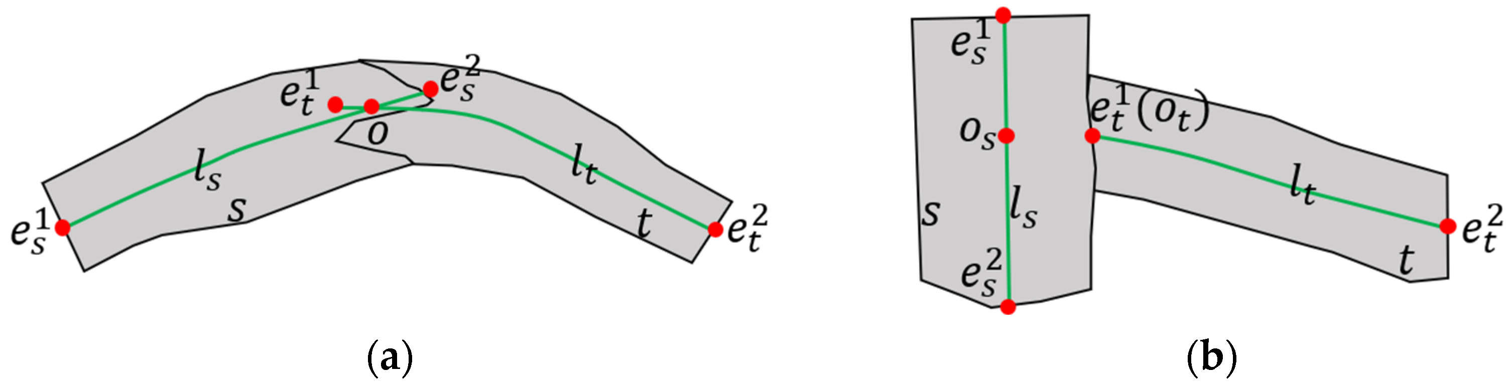
3.3.1. Control Point Searching

Starting from a set $S_C$ which contains all the clusters obtained after applying the perceptual grouping process in Section 3.2, the polynomial curve fitting [17] method is applied to each cluster $s(s\in S_C)$ using pixel coordinates in $s$ as observation data, and then, a thinning curve $l_s$ can be drawn. Let $E_s=\{e_s^1,e_s^2\}$ be the set of two endpoints of $l_s$, and $N_s$ be the needed set of nodes related to $s$. Due to the fact that endpoints are undoubtedly one of the used nodes for the spline model, $N_s$ is initialized by $N_s=E_s$. If $s$ has no neighboring cluster, it is certain that $l_s$ is the final extracted centerline. In the case that neighboring clusters exist, Figure 6 presents a schematic diagram for extracting the nodes. More specifically, the connection nodes for two adjacent clusters ($s$ and $t$) are further determined by the following two rules:

(1)

In the case that $l_s$ and $l_t$ have intersection points, the midpoint $o$ of intersections is added to the sets $N_s$ and $N_t$.

(2)

In the case that $l_s$ and $l_t$ have no intersection points, determine the two closest points $\{o_s,o_t\}$ between $s$ and $t$ first. If $o_s\in E_s$ and $o_t\notin E_t$, add the point $o_t$ to the set $N_s$ and $N_t$. Conversely, if $o_s\notin E_s$ and $o_t\in E_t$, put the point $o_s$ into the set $N_s$ and $N_t$. For all other cases, the midpoint between $o_s$ and $o_t$ is the determined connection node and is added to the sets $N_s$ and $N_t$.

By checking all the road clusters and their neighbors in the map, a set of nodes can be achieved with $N={\displaystyle {\cup }_{s\in S_c}{N}_s}$. To merge nodes that are close to each other in $N$, agglomerative hierarchical clustering [23] is then applied. That method starts by treating each node as a singleton cluster. Next, pairs of clusters are successively merged until all their Euclidean distances are smaller than a threshold of $T_n$ pixels.

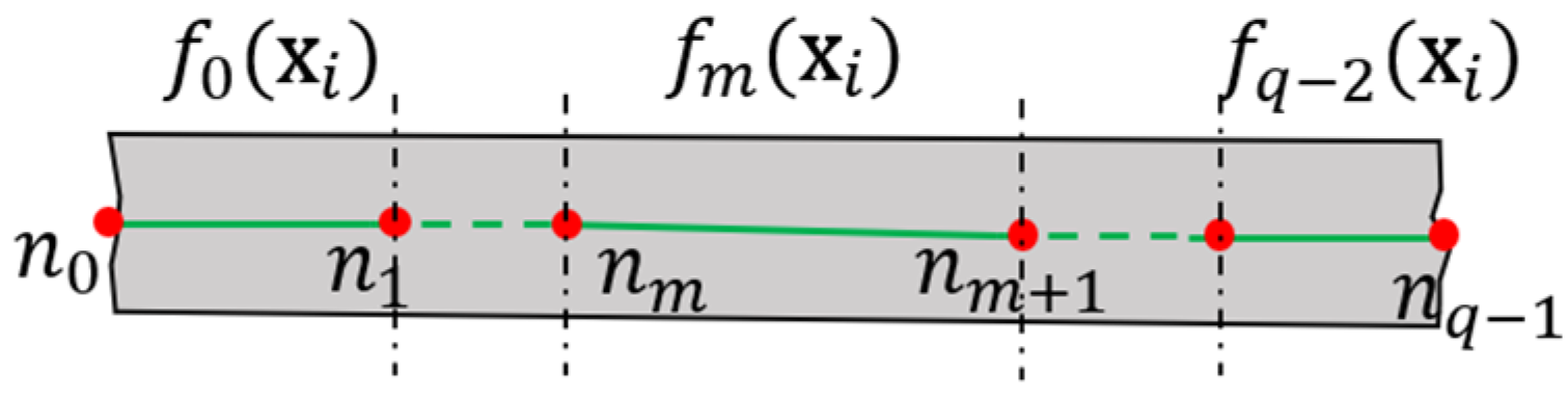
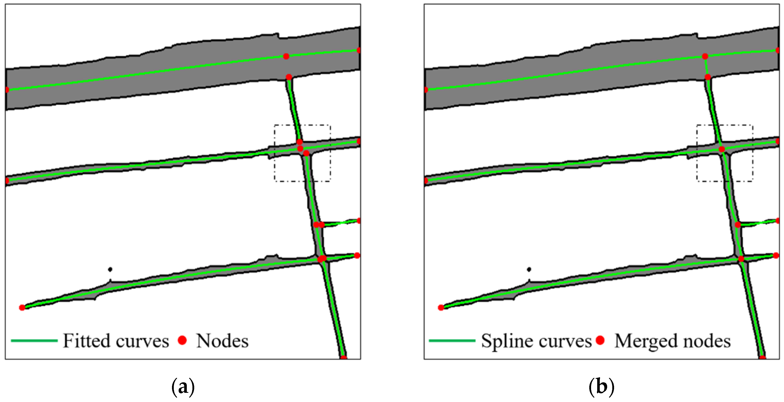
3.3.2. Spline Fitting

Once the final nodes are achieved, road centerlines are extracted based on the spline fitting. Let ${{\rm N}}_s=\{n_0,n_1,\mathrm{\dots },n_{q-1}\}$ represent $q$ sorted nodes in a cluster $s(s\in S_C)$ according to pixel rows or columns. Supposing that $f_m(x_i)={\displaystyle {\sum }_{j=0}^{\beta }{\omega }_j{x}_i^j}={\omega }^T{x}_i$ where $x_i=(x_i^0,x_i^1,\mathrm{\dots },x_i^{\beta })$ is the polynomial function denoting the curve between nodes $n_m$ and $n_{m+1}(m=0,1,\mathrm{\dots },q-2)$, each curve must be made to pass through its nodes and minimize the residual sum of squares (RSS), i.e.,

$$\begin{array}{l}\underset{\omega }{\min }{{\displaystyle {\sum }_{i=1}^k\left[y_i-f_m(x_i)\right]}}^2\\ s.t.f_m(x_{n_m})=y_{n_m},f_m(x_{n_{m+1}})=y_{n_{m+1}}\end{array}$$

(4)

where $x_i$ and $y_i$ denote coordinates of pixels between nodes $n_m$ and $n_{m+1}$ in $s$, $k$ is the number of pixels, and $\beta$ is the polynomial order which is set to 3. This is an optimization problem with equality constraints, and thus, can be solved using the general Lagrange multiplier method [24]. In order to illustrate the proposed centerline extraction method, Figure 7 presents a schematic diagram for spline fitting on a road cluster. It is worth mentioning that two nodes will be connected with a straight line if there are no pixels for fitting between these two nodes in a cluster, or the root-mean-square error (RMSE) of fitting is larger than the mean road width $w(s)$ of the cluster.

Figure 8 presents an example for the proposed centerline extraction method. In Figure 8a, the fitted polynomial curves on each road cluster are labelled as green lines and the extracted nodes are marked with red dots. As shown in Figure 8b, nodes in the dashed box are merged into one node using the agglomerative hierarchical clustering method. Figure 8b also shows the final centerlines passing through merged nodes in the image based on the proposed spline fitting method.

4. Experimental Results

4.1. Dataset Description and Result Evaluation

In order to access the effectiveness of the proposed methodology, six different segmented road maps from real satellite images were tested. More specifically, in our work, test images 1 and 2 were optical images from Worldview-2, and a method from [16] was used to obtain the segmented road binary map. In [16], a road segmentation model is proposed which combines the adversarial networks with multiscale context aggregation. Furthermore, test images 3 and 4 were TerraSAR-X and Radarsat-2 images, and roads are first segmented by the method in [17], which are based on multiplicative Duda operation and morphological profiles of path openings. Test images 5 and 6 were selected from the DeepGlobe road dataset [25] where roads were labelled manually.

To evaluate the proposed method, the results achieved in this paper are analyzed visually and numerically. For the visual analysis, the centerline extraction results are roughly evaluated by comparing the length, shape, junction, and connectedness of roads with the reference road centerlines. The reference centerlines were ground truth data generated manually from the original satellite images.

For the numerical comparison analysis, completeness (CP), correctness (CR), and quality (QL) are computed using the reference data based on the evaluation method in [26]. According to the principles in [26], a buffer is set to determine which parts of one road network are considered to be matched with the other. In this paper, the buffer is set to 5 pixels. In detail, the aforementioned evaluation indexes are given by

$$\{\begin{array}{l}CP = \frac{TP}{TP + FN}\\ CR = \frac{TP}{TP + FP}\\ QL = \frac{TP}{TP + FP + FN} = \frac{CP \times CR}{CP + CR - CP \times CR}\end{array}.$$

(5)

where TP is the length of the extracted centerlines that matched with the reference data, FP is the length of extracted centerlines that do not match reference data, and FN denotes the length of reference centerlines that do not match extracted centerlines. The QL index can be treated as a general index which combines CP and CR. It can be also inferred that the values of all the three indexes range from 0 to 1. A larger value means that the extraction result is closer to the reference data.

Considering that the input segmented road map may have false and missing parts, its three quantitative indexes, mentioned above, can also be computed using the evaluation method in [26] by matching the ground truth data with the manually labelled centerlines of the input segmented road map. That is to say, a centerline is manually generated for each road segment of the input road map, and then the CP, CR, and QL values are calculated by comparing them with ground truth data. The accuracy for six input segmented road maps can be found in tables in Section 4.2.

In terms of computational efficiency, the total execution time (ET) of centerline extraction using different methods is also proposed in this paper. All the experiments were conducted on a computer with an AMD R7-4800H processor and 16GB RAM using MATLAB codes.

4.2. Experimental Results and Comparisons

This section shows the results achieved by the proposed method and four existing methods. The parameter setting used for the proposed method is also presented. In this section, the experimental results for segmented road maps from optical images are presented in Section 4.2.1. Section 4.2.2 proposes the results obtained using the segmented road map from SAR images. Next, the results obtained from labelled road images are shown in Section 4.2.3. Finally, Section 4.2.4 presents the comparison results of different methods based on a McNemar test.

To verify the performance, the proposed method is compared with four state-of-the-art methods. The first one is the classic morphological thinning (MT) algorithm [5]. The second is based on the Zhang–Suen thinning (ZST) algorithm [27]. Miao et al. [7] introduced a method using tensor voting and multivariate adaptive regression splines (MARS), which is the third one for comparison. The last one is the method presented by Cheng et al. [8] which utilized approaches of tensor voting and non-maximum suppression (NMS).

For the parameter setting, the proposed method mainly depends on three parameters, namely: diameter $D$ of the window in Section 3.1; threshold $T_{\lambda }$ of the collinearity degree in Section 3.2.3; threshold $T_n$ for clustering nodes in Section 3.3.1. The parameters used in the 6 test images have been listed in

Table 1. Parameters used in the test images.

Test Images	$\mathit{D}$ (pixels)	${\mathit{T}}_{\mathit{\lambda }}$	${\mathit{T}}_{\mathit{n}}\left(\mathbf{pixels}\right)$
1	101	0.01	10
2	101	0.001	30
3	61	0.001	20
4	61	0.005	10
5	51	0.001	10
6	51	0.005	20

. In conclusion, it is suggested that $D$ should be slightly larger than the maximum width of the road in the image. Parameter $T_{\lambda }$ is usually a small number near zero. The continuity grouping step can be ignored when $T_{\lambda }$ is set to zero. $T_n$ is determined empirically to merge close nodes. More details for the analysis of these parameters can be found in Section 5.

4.2.1. Cases for Optical Images

For the experiments on optical data, two TrueColor images, also known as RGB images, with 0.5 m spatial resolution collected from the Worldview-2 sensor, are used. The two regions are located in Wuzhen, Zhejiang, China. It is important to note that both test images 1 and 2 are shown in Figure 9a and Figure 10a, and contain different road segments with large differences in width. The segmented road maps from test images 1 and 2 are presented in Figure 9b and Figure 10b along with their reference centerline data in Figure 9c and Figure 10c. The centerline extraction results using the proposed method and four existing methods are also displayed in Figure 9 and Figure 10.

Table 2. Quantitative indexes of centerline extraction in test images 1 and 2 with different methods.

Test Images (Size)	Quantitative Indexes	Accuracy of Input Road Map	MT	ZST	MARS	NMS	Proposed Method
1 (650 × 650)	CP (%)	86.94	80.22	83.36	82.67	79.61	84.78
	CR (%)	98.82	89.36	87.73	91.84	87.42	94.73
	QL (%)	86.05	73.22	74.66	77.01	71.43	80.97
	ET (s)	-	0.01	1.87	98.79	223.01	4.55
2 (2500 × 2500)	CP (%)	92.63	87.46	86.78	82.49	83.85	84.84
	CR (%)	96.03	84.36	83.64	81.39	87.33	87.23
	QL (%)	89.21	75.26	74.19	69.40	74.76	75.47
	ET (s)	-	0.16	39.07	745.63	834.17	25.03

presents the quantitative indexes of evaluation for the two test images.

As can be observed from the results in Figure 9, the proposed method has the best performance for the marked junction area. The other four existing methods fail to extract an accurate junction, which leads to lower values in terms of quantitative indexes compared with the proposed method. In Figure 10, for test image 2, it can be also seen that the approaches of MT, ZST, and MARS bring loops when the irregular edges and holes exist on the segmented road region. The NMS method achieves the best result in terms of CR, although it fails to link the centerlines well in some intersection areas. In addition, one can also notice that the execution time of MARS and NMS is much longer than the other methods. This happens because tensor voting is a time-consuming process, especially when the road width of the image is large, and the large value should be set for the parameter of the voting scale. Overall, our proposed method provides results with better QL and acceptable ET.

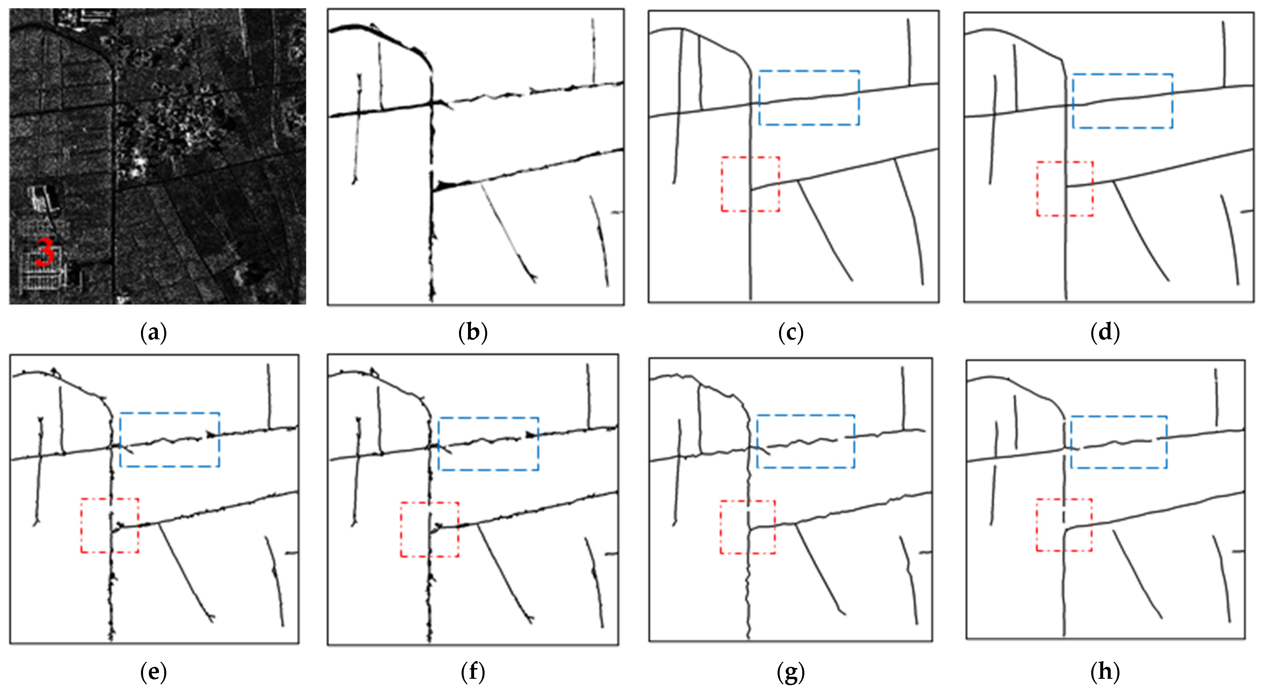
4.2.2. Cases for SAR Images

In the case of using SAR data, test image 3 with 1 m spatial resolution obtained from the TerraSAR-X senor, and test image 4 with 2 m resolution obtained from Radarsat-2 sensor, are used. The original SAR images and the segmented road map are presented in Figure 11 and Figure 12. As before, extracted road centerlines using different methods are marked with black lines in the experimental results. The corresponding evaluation indexes for test images 3 and 4 are shown in

Table 3. Quantitative indexes of centerline extraction in test images 3 and 4 with different methods.

Test Images (Size)	Quantitative Indexes	Accuracy of Input Road Map	MT	ZST	MARS	NMS	Proposed Method
3 (860 × 860)	CP (%)	92.12	90.46	90.23	78.92	86.53	89.37
	CR (%)	99.05	77.45	76.83	82.05	94.96	94.47
	QL (%)	91.31	71.60	70.93	67.30	82.73	84.93
	ET (s)	-	0.01	1.36	86.07	128.76	12.38
4 (1941 × 1585)	CP (%)	70.45	68.33	67.30	64.28	65.89	68.02
	CR (%)	77.76	64.06	65.54	67.78	76.22	74.73
	QL (%)	58.63	49.39	49.71	49.24	54.65	55.30
	ET (s)	-	0.03	6.15	247.85	397.56	43.18

.

Due to the effect of multiplicative speckle noise, the segmented road map from SAR images may contain more false and missing road parts, together with irregular edges, compared with those from optical data, as shown in Figure 11b and Figure 12b. These irregular edges result in burrs when the MT method is applied. It can be explained by the topological equivalence principle during MT operation, which leads to better results for regular road segments, but is not good for irregular ones. It can be also noticed that a similar problem exists in the case of using the ZST method, which leads to a low value in the CR index. Although the NMS method shows the best performance in terms of CR among these methods, experiments still demonstrate the advantages of the proposed method when both QL and ET are considered. Moreover, the proposed method also shows the ability to connect small gaps, according to the blue box area in Figure 11. This is done by adjusting the parameter $T_n$ when merging close nodes in Section 3.3.1. For test image 4, although the extraction quality of the input road map is not high, the centerline extraction using the proposed method only brings about 3.3% quality loss.

4.2.3. Cases for Labelled Road Images

For the experiments using manually labelled road maps, two test images selected from the labelled training data of the DeepGlobe road dataset [25] are used. The accuracy of input maps can be considered as 100%. As can be seen in Figure 13b and Figure 14b, road segments are much more regular and smoother than that in the previous test images. Test image 5 is selected for testing the centerline extraction performance in mountainous areas where roads have a large curvature. As for test image 6, it includes complex road networks where many junctions exist, and the width of the road has a large change.

For test image 5, it is clear to note that the proposed method, and all the other four methods, demonstrate a good performance according to the experimental results in

Table 4. Quantitative indexes of centerline extraction in test images 5 and 6 with different methods.

Test Images (Size)	Quantitative Indexes	Accuracy of Input Road Map	MT	ZST	MARS	NMS	Proposed Method
5 (1024 × 1024)	CP (%)	100	99.52	99.60	93.83	99.21	97.30
	CR (%)	100	99.07	98.87	94.89	98.76	96.77
	QL (%)	100	98.61	98.48	89.31	97.99	94.24
	ET (s)	-	0.01	1.49	91.71	75.73	7.60
6 (1024 × 1024)	CP (%)	100	95.34	91.97	70.45	80.54	95.29
	CR (%)	100	95.28	89.10	72.27	81.26	94.90
	QL (%)	100	91.03	82.67	55.46	67.93	90.64
	ET (s)	-	0.04	5.52	1849.60	2125.40	10.99

and Figure 13. Nevertheless, the MT approach has the shortest execution time and highest QL value. That indicates that MT should be the best choice for centerline extraction, on the condition that the road network is simple, and the road width is small. In the case of test image 6, the MT method still shows the best results and fastest speed for the quantitative indexes compared with other methods; however, it can be found that our proposed method provides more precise road junctions by comparing the experimental results with the reference data. Taking the intersections that are perpendicular to each other as an example, the extraction results of the proposed method can better ensure the vertical relationship between road centerlines, whereas the MT method and other methods cannot. To sum up, experiments show that the MT method should take priority over other approaches when the segmented roads are smooth and narrow, whereas the proposed method has advantages in constructing accurate road junctions when roads are complex and wide. Combined with the previous four test images, the experiments also emphasize the stability and flexibility of the proposed method. Thus, regardless of whether the segmented road map is disturbed by noise or not, our proposed method demonstrates a good performance in centerline extraction.

4.2.4. Comparisons of Different Methods

In order to statistically test whether there is any significant difference between the extraction results of the proposed method and other four existing methods, a McNemar test [28] is performed. The McNemar test is a nonparametric test which focuses on the binary distinction between correct and incorrect class assignments. This test is conducted using the standardized normal test statistic

$$z=\frac{f_{12}-f_{21}}{\sqrt{f_{12}+f_{21}}}.$$

(6)

where $f_{12}$ and $f_{21}$ denote the number of sampled pixels that are correctly classified with one method, and are incorrectly classified with the other method. Based on [28], the square of $z$ follows a chi-squared (${\chi }^2$) distribution with one degree of freedom. Thus, it can be concluded that the difference between the extraction results of the two approaches is statistically significant ($p<0.05$) if $\left|z\right|$ is greater than 1.96.

In this paper, the sampled pixels for statistical analysis are composed of road pixels and non-road pixels. The sampled road pixels are selected from road segments in the ground truth data. Since non-road pixels occupy a large proportion of the image, and most of the non-road pixels are correctly classified as non-road pixels, it is only necessary to combine the wrongly extracted parts of the extraction results, using the two methods, to be compared against the sampled non-road pixels. More specifically, according to the matching rules in [26], the extracted centerlines that do not match reference data are treated as the wrongly extracted parts in an extraction result. Through analyzing the sampled pixels in the six test images,

Table 5. Results of the statistical comparison ($z$ values) between the proposed method and the four existing methods using the McNemar tests. The positive values represent the former method having a higher extraction quality than the latter.

Test Images	Proposed Method vs. MT	Proposed Method vs. ZST	Proposed Method vs. MARS	Proposed Method vs. NMS	MT vs. ZST	MT vs. MARS	MT vs. NMS	ZST vs. MARS	ZST vs. NMS	MARS vs. NMS
1	10.22	9.72	7.11	11.97	−1.66	−2.80	2.18	−3.27	4.49	5.96
2	3.92	8.80	25.58	0.71	9.03	28.18	4.42	20.93	−10.52	−28.50
3	21.57	24.09	23.93	2.84	2.11	2.60	−18.84	1.14	−21.06	−20.26
4	20.47	22.39	21.13	8.34	−2.21	2.78	−32.13	4.01	−33.38	−32.17
5	−11.82	−10.75	8.51	−10.45	2.29	19.41	4.04	18.36	1.09	−18.81
6	−0.20	20.08	61.02	40.93	21.07	62.82	42.94	46.82	24.00	−28.78

presents the $z$ values of the McNemar tests between every two mentioned centerline extraction methods in this paper.

According to the McNemar tests, the results of the proposed method are significantly more accurate than those derived from the other four state-of-the-art methods in test images 1, 3, and 4 ($p<0.05$). There is an exception in test image 2 where it indicates that the difference in the accuracy of the extractions derived from the proposed method and the NMS method are not statistically significant ($p<0.05$). For the labelled road maps of test images 5 and 6, there are significant differences ($\left|z\right|>1.96$) at a 95% confidence level when the MT method is compared with the other four methods, except for the case of the proposed method vs. the MT method in test image 6. In conclusion, the proposed method significantly outperforms the other four existing methods for mapping road centerlines from noise-disturbed images, such as SAR images. Although the method in this paper may not have had the best extraction quality for regular segmented road maps, it has advantages in constructing more precise junctions, while maintaining a high extraction quality, by visually comparing junction shapes in the experimental results.

5. Discussion

This section presents the parameter sensitivity analysis of the proposed method using the test images. These parameters include the diameter $D$ in the stage of the RoC operation, threshold $T_{\lambda }$ in the stage of perceptual grouping, and threshold $T_n$ in the stage of spline fitting.

5.1. Analysis for RoC Detector

Concerning the RoC detector, the diameter $D$ of the sliding window is a key parameter. Undoubtedly, the chosen value of $D$ should ensure the accuracy of the road direction and width feature extraction as much as possible. In order to present the effects of parameter $D$, the quantitative indexes of results using the proposed method with different values of $D$ in test images 2 and 6 are computed and compared. As illustrated in Figure 15, for the two test images, all the three indexes are at low values when $D$ is small. As $D$ increases, the quantitative indexes also tend to increase and then reach stable values. Empirically, the turning point to reach a plateau is on the condition that $D$ reaches the maximum width of the road in the image. Thus, it is suggested that $D$ should be set based on prior knowledge of the maximum road width; however, parameter $D$ should not be too large. If the value of $D$ is too large, it may lead to poor detection performance because the sliding window may pass through two or more parallel road segments.

Additionally, the influence of the MRF method mentioned in Section 3.1 is introduced. Using the proposed RoC detector, roads are originally segmented into several classes according to the orientation feature. The application of MRF aims to merge isolated road pixels, which have different direction features, from surround pixels using the local spatial relationship.

Table 6. Quantitative indexes of centerline extraction in test images 2, 4, and 6, using the proposed method with and without the MRF procedure.

Test Images (Size)	Proposed Method	Quantitative Indexes
		CP (%)	CR (%)	QL (%)	ET (s)
2 (2500 × 2500)	with MRF	84.84	87.23	75.47	25.03
	without MRF	84.03	85.73	73.72	25.98
4 (1941 × 1585)	with MRF	68.02	74.73	55.30	43.18
	without MRF	64.59	70.09	50.64	74.98
6 (1024 × 1024)	with MRF	95.29	94.90	90.64	10.99
	without MRF	95.07	94.12	89.74	10.69

presents the comparison results in the case of using the proposed method with and without the MRF procedure in test images 2, 4, and 6. It can be seen that the usage of MRF is able to slightly improve the centerline extraction results in terms of the indexes of CP, CR, and QL. By comparing the ET for test images 2 and 6, it is noted that the time cost of MRF is almost negligible; however, the case for test image 4 is an exception, where the ET of using the proposed method without MRF is significantly longer. This can be explained by the fact that the roads in test image 4 are noticeably irregular, and thus, the number of road clusters in $S$, after direction grouping, is quite large if the MRF step is not included. The computational complexity of Algorithm 1 for perceptual grouping in Section 3.2 is proportional to the number of road clusters in the input $S$. The application of MRF is beneficial to reduce the number of road clusters in advance.

5.2. Analysis for Perceptual Grouping

With regard to the stage of perceptual grouping for the proposed method, three parameters are mainly involved including $T_H$ for proximity grouping, along with $T_{\lambda }$ and $T_w$, for continuity grouping. Threshold $T_H$ can be set adaptively using the corresponding road width value detected by the RoC operation. Threshold $T_w$ is recommended to be set to a single lane width; therefore, threshold $T_{\lambda }$ is the one that remains to be determined manually in practical application. In order to evaluate the parameter sensitivity, experiments with a different threshold $T_{\lambda }$ is conducted. Test images 2 and 6 are used, and the results are shown in Figure 16. When threshold $T_{\lambda }$ is 0, Equation (3) cannot be satisfied and that means the continuity grouping step will not be executed. It can be observed that a very small number greater than 0 can slightly improve the centerline extraction accuracy; however, when the value of $T_{\lambda }$ increases, the inflection point will appear, and the performance of the method will deteriorate sharply. It is clear that the location of the inflection point is not fixed, and it may vary from image to image. As a consequence, it is suggested to set $T_{\lambda }$ to zero or to try using a very small number empirically, in practice.

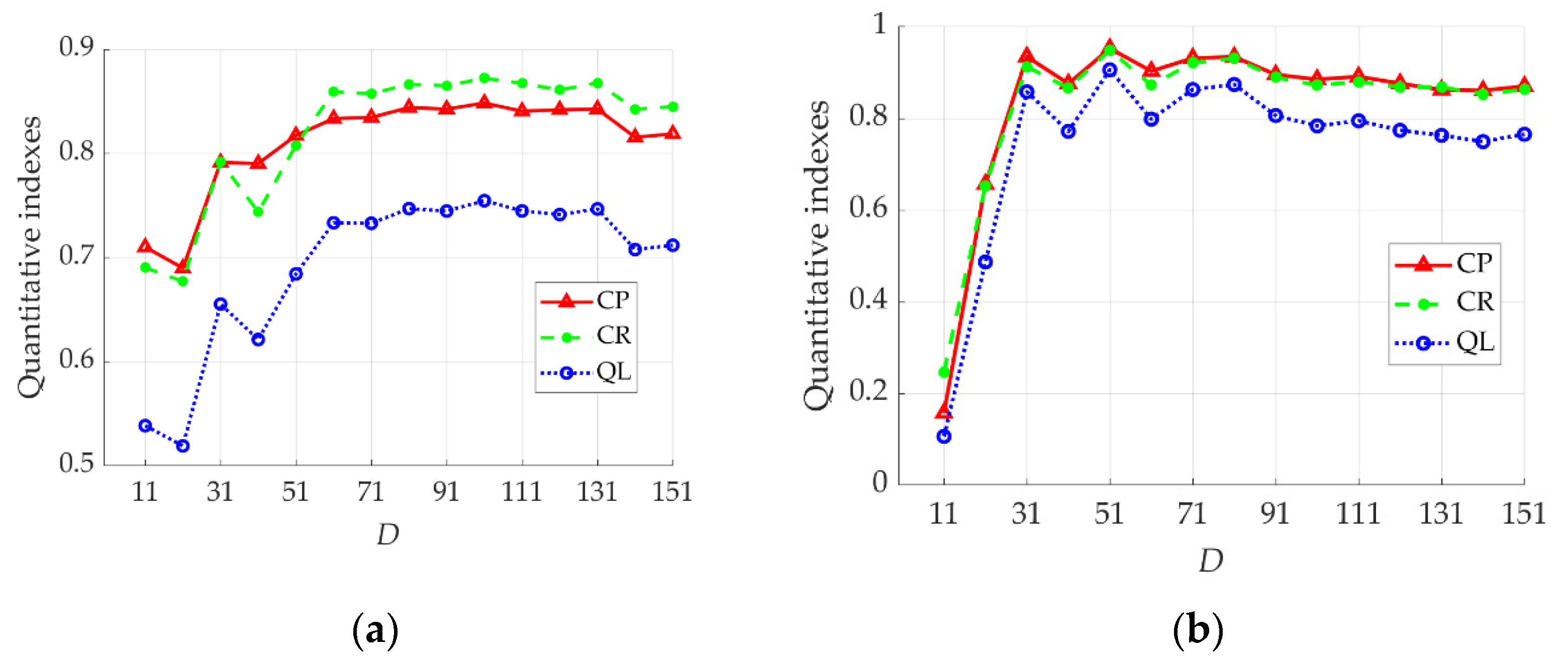
5.3. Analysis for Spline Fitting

For the spline fitting stage of the proposed method, threshold $T_n$ determines the minimum distance between nodes. If the Euclidean distances between two nodes is smaller than $T_n$, they will be replaced by the midpoint of the two nodes. Generally, a $T_n$ value that is too small may lead to the generation of small burrs at the spline junctions. When threshold $T_n$ is too large, nodes may deviate from the centerline position and further cause an inaccurate centerline extraction. The experimental results in Figure 17 illustrate the effects of parameter $T_n$. Taking Figure 17a as an example, when $T_n$ is in the range of 0 to 40, QL is able to stabilize at around 75%; however, as the value of $T_n$ is greater than 40, there is a significant drop in QL. Experimental results show that $T_n$ should not be set to a large number. Empirically, it should not exceed the maximum road width in the image.

6. Conclusions

In this paper, a general method for road centerline extraction from remote sensing images is proposed based on perceptual grouping and spline fitting. The proposed method is suitable for noisy data and is competitive in computational efficiency. Furthermore, experiments presented the merits of the proposed method in junction construction, gap connection, and the adaptability for road segmentation resulting from different sources. From the results of the quantitative analysis, the following conclusions can be drawn. Firstly, the completeness and correctness of extracted centerlines using the proposed method can be over 84% and 68%, respectively, on the test images. Secondly, for the segmented road maps obtained by machine recognition, the proposed method has the best QL indexes. Moreover, the McNemar tests demonstrate that there are significant differences at a 95% confidence level when the proposed method is compared with the methods of MT, ZST, MARS, and NMS, except for the case of the proposed method vs. NMS in test image 2. Thirdly, for the manually labelled road maps, the MT method shows the best performances in terms of both accuracy and execution time. The advantage of our method is that it can provide a more precise road junction shape, and is not too different from the MT method in terms of accuracy.

However, it can also be noted that some algorithm parameters of the proposed method have to be determined manually according to the available prior knowledge of image resolution, and the maximum road width based on practical applications. Thus, it is desirable to develop an automatic threshold determination approach for parameter setting in the future. Nevertheless, experimental results indicate that the proposed method has excellent application potentials, such as road data update, the fusion of road networks, and the road vectorization and generalization in GISs.

References

1. Bulatov, D.; Häufel, G.; Pohl, M. Vectorization of road data extracted from aerial and uav imagery. Int. Arch. Photogramm. Remote Sens. Spat. Inf. Sci. 2016, 41, 567–574. [Google Scholar] [CrossRef] [Green Version]
2. Zhou, J.; Bischof, W.F.; Caelli, T. Road tracking in aerial images based on human-computer interaction and Bayesian filtering. Isprs J. Photogramm. Remote Sens. 2006, 61, 108–124. [Google Scholar] [CrossRef] [Green Version]
3. Cheng, J.; Gao, G. Parallel particle filter for tracking road centrelines from high-resolution SAR images using detected road junctions as initial seed points. Int. J. Remote Sens. 2016, 37, 4979–5000. [Google Scholar] [CrossRef]
4. Dal Poz, A.P.; Zanin, R.B.; do Vale, G.M. Automated Extraction of Road Network from Medium- and High-Resolution Images. Pattern Recognit. Image Anal. Adv. Math. Theory Appl. 2006, 16, 239–248. [Google Scholar] [CrossRef]
5. Wei, Y.; Zhang, K.; Ji, S. Simultaneous Road Surface and Centerline Extraction from Large-Scale Remote Sensing Images Using CNN-Based Segmentation and Tracing. IEEE Trans. Geosci. Remote Sens. 2020, 58, 8919–8931. [Google Scholar] [CrossRef]
6. Sujatha, C.; Selvathi, D. Connected component-based technique for automatic extraction of road centerline in high resolution satellite images. Eurasip J. Image Video Process. 2015, 2015, 8. [Google Scholar] [CrossRef] [Green Version]
7. Miao, Z.; Shi, W.; Zhang, H.; Wang, X. Road Centerline Extraction from High-Resolution Imagery Based on Shape Features and Multivariate Adaptive Regression Splines. IEEE Geosci. Remote Sens. Lett. 2013, 10, 583–587. [Google Scholar] [CrossRef]
8. Cheng, G.; Zhu, F.; Xiang, S.; Wang, Y.; Pan, C. Accurate urban road centerline extraction from VHR imagery via multiscale segmentation and tensor voting. Neurocomputing 2016, 205, 407–420. [Google Scholar] [CrossRef] [Green Version]
9. Zhou, T.; Sun, C.; Fu, H. Road Information Extraction from High-Resolution Remote Sensing Images Based on Road Reconstruction. Remote Sens. 2019, 11, 79. [Google Scholar] [CrossRef] [Green Version]
10. Sironi, A.; Turetken, E.; Lepetit, V.; Fua, P. Multiscale Centerline Detection. IEEE Trans. Pattern Anal. Mach. Intell. 2016, 38, 1327–1341. [Google Scholar] [CrossRef] [Green Version]
11. Wei, Y.; Hu, X.; Gong, J. End-to-End road centerline extraction via learning a confidence map. In Proceedings of the 2018 10th IAPR Workshop on Pattern Recognition in Remote Sensing, Beijing, China, 19–20 August 2018. [Google Scholar]
12. Yang, X.; Li, X.; Ye, Y.; Lau, R.Y.K.; Zhang, X.; Huang, X. Road Detection and Centerline Extraction Via Deep Recurrent Convolutional Neural Network U-Net. IEEE Trans. Geosci. Remote Sens. 2019, 57, 7209–7220. [Google Scholar] [CrossRef]
13. Negri, M.; Gamba, P.; Lisini, G.; Tupin, F. Junction-aware extraction and regularization of urban road networks in high-resolution, SAR images. IEEE Trans. Geosci. Remote Sens. 2006, 44, 2962–2971. [Google Scholar] [CrossRef]
14. Xiao, F.; Chen, Y.; Tong, L.; Yang, X. Coherence estimation in the low-backscattering area using multitemporal TerraSAR-X images and its application on road detection. In Proceedings of the 2017 IEEE International Geoscience and Remote Sensing Symposium (IGARSS), Fort Worth, TX, USA, 23–28 July 2017; pp. 898–901. [Google Scholar]
15. Zhang, Z.; Zhang, X.; Sun, Y.; Zhang, P. Road Centerline Extraction from Very-High-Resolution Aerial Image and LiDAR Data Based on Road Connectivity. Remote Sens. 2018, 10, 1284. [Google Scholar] [CrossRef] [Green Version]
16. Li, Y.; Peng, B.; He, L.; Fan, K.; Tong, L. Road Segmentation of Unmanned Aerial Vehicle Remote Sensing Images Using Adversarial Network with Multiscale Context Aggregation. IEEE J.-Stars 2019, 12, 2279–2287. [Google Scholar] [CrossRef]
17. Xiao, F.; Tong, L.; Luo, S. A Method for Road Network Extraction from High-Resolution SAR Imagery Using Direction Grouping and Curve Fitting. Remote Sens. 2019, 11, 2733. [Google Scholar] [CrossRef] [Green Version]
18. Tarabalka, Y.; Fauvel, M.; Chanussot, J.; Benediktsson, J.A. SVM- and MRF-Based Method for Accurate Classification of Hyperspectral Images. IEEE Geosci. Remote Sens. Lett. 2010, 7, 736–740. [Google Scholar] [CrossRef] [Green Version]
19. Stilla, U.; Michaelsen, E.; Soergel, U.; Schulz, K. Perceptual grouping of regular structures for automatic detection of man-made objects. In Proceedings of the 23rd International Geoscience and Remote Sensing Symposium (IGARSS 2003), Toulouse, France, 21–25 July 2003; pp. 3525–3527. [Google Scholar]
20. He, L.; Chao, Y.; Suzuki, K. A Run-Based Two-Scan Labeling Algorithm. IEEE T Image Process. 2008, 17, 749–756. [Google Scholar]
21. Avbelj, J.; Müller, R.; Bamler, R. A Metric for Polygon Comparison and Building Extraction Evaluation. IEEE Geosci. Remote Sens. Lett. 2015, 12, 170–174. [Google Scholar] [CrossRef] [Green Version]
22. Jiang, M.; Miao, Z.; Gamba, P.; Yong, B. Application of Multitemporal InSAR Covariance and Information Fusion to Robust Road Extraction. IEEE Trans. Geosci. Remote 2017, 55, 3611–3622. [Google Scholar] [CrossRef]
23. Marcal, A.R.S.; Castro, L. Hierarchical clustering of multispectral images using combined spectral and spatial criteria. IEEE Geosci. Remote Sens. Lett. 2005, 2, 59–63. [Google Scholar] [CrossRef]
24. Yang, X. Nature-Inspired Optimization Algorithms; Academic Press: Cambridge, MA, USA, 2020. [Google Scholar]
25. Demir, I.; Koperski, K.; Lindenbaum, D.; Pang, G.; Huang, J.; Basu, S.; Hughes, F.; Tuia, D.; Raskar, R. DeepGlobe 2018: A Challenge to Parse the Earth through Satellite Images. In Proceedings of the 2018 IEEE/CVF Conference on Computer Vision and Pattern Recognition Workshops (CVPRW), Salt Lake City, UT, USA, 18–22 June 2018; pp. 172–181. [Google Scholar]
26. Wiedemann, C.; Heipke, C.; Mayer, H.; Jamet, O. Empirical Evaluation Of Automatically Extracted Road Axes. Empir. Eval. Tech. Comput. Vis. 1998, 12, 172–187. [Google Scholar]
27. Chen, B.; Ding, C.; Ren, W.; Xu, G. Extended Classification Course Improves Road Intersection Detection from Low-Frequency GPS Trajectory Data. ISPRS Int. J. Geo-Inf. 2020, 9, 181. [Google Scholar] [CrossRef] [Green Version]
28. Foody, G.M. Thematic map comparison. Photogramm. Eng. Remote Sens. 2004, 70, 627–633. [Google Scholar] [CrossRef]
Figure 1. Diagrammatic sketches of the proposed method, validation, and analysis processes.
Remotesensing 14 02074 g001
Figure 2. RoC detector. (a) Sketch map of RoC detector (N = 8). (b) Length ratios for sampled horizontal and vertical road pixels at different directions.
Remotesensing 14 02074 g002
Figure 3. Detected feature maps from a sample road binary map. (a) Detected direction map (N = 8). (b) Refined direction map using MRF. (c) Detected width map.
Remotesensing 14 02074 g003
Figure 4. A sketch map for the Hausdorff distance where A, B, and C represent three different road clusters, and w(B) is the mean value of width feature for all pixels in B.
Remotesensing 14 02074 g004
Figure 5. An example for object-based perceptual grouping. (a) A detected direction map. (b) Direction grouping result obtained from (a) different clusters divided by edges, and (c) proximity grouping result using (b) as an input. Red cluster A and blue cluster B are two adjacent clusters that satisfy continuity rules. (d) Continuity grouping result using (c) as an input.
Remotesensing 14 02074 g005
Figure 6. A schematic diagram for extracting the nodes from adjacent clusters. (a) A case when l s and l t have intersection points. (b) A case when l s and l t do not have intersection points.
Remotesensing 14 02074 g006
Figure 7. A schematic diagram for spline fitting using extracted control points on a road cluster.
Remotesensing 14 02074 g007
Figure 8. An example for spline fitting. (a) Fitted polynomial curves and detected nodes on each cluster. (b) Spline fitting based on merged nodes.
Remotesensing 14 02074 g008
Figure 9. Experimental results for test image 1. (a) Original optical image. (b) Segmented road map. (c) Reference of the centerline map. (d) Result of the proposed method. (e) Result of the MT method. (f) Result of the ZST method. (g) Result of the MARS method. (h) Result of the NMS method.
Remotesensing 14 02074 g009
Figure 10. Experimental results for test image 2. (a) Original optical image. (b) Segmented road map. (c) Reference centerline map. (d) Result of the proposed method. (e) Result of the MT method. (f) Result of the ZST method. (g) Result of the MARS method. (h) Result of the NMS method.
Remotesensing 14 02074 g010
Figure 11. Experimental results for test image 3. (a) Original SAR image. (b) Segmented road map. (c) Reference centerline map. (d) Result of the proposed method. (e) Result of the MT method. (f) Result of the ZST method. (g) Result of the MARS method. (h) Result of the NMS method.
Remotesensing 14 02074 g011
Figure 12. Experimental results for test image 4. (a) Original SAR image. (b) Segmented road map. (c) Reference centerline map. (d) Result of the proposed method. (e) Result of the MT method. (f) Result of the ZST method. (g) Result of the MARS method. (h) Result of the NMS method.
Remotesensing 14 02074 g012
Figure 13. Experimental results for test image 5. (a) Original optical image. (b) Labelled road map. (c) Reference centerline map. (d) Result of the proposed method. (e) Result of the MT method. (f) Result of the ZST method. (g) Result of the MARS method. (h) Result of the NMS method.
Remotesensing 14 02074 g013
Figure 14. Experimental results for test image 6. (a) Original optical image. (b) Labelled road map. (c) Reference centerline map. (d) Result of the proposed method. (e) Result of the MT method. (f) Result of the ZST method. (g) Result of the MARS method. (h) Result of the NMS method.
Remotesensing 14 02074 g014
Figure 15. The quantitative indexes (CP, CR, QL) versus the diameter D of the sliding window. (a) Results for test image 2. (b) Results for test image 6.
Remotesensing 14 02074 g015
Figure 16. The quantitative indexes (CP, CR, QL) versus the threshold T λ in the experiments. (a) Results for test image 2. (b) Results for test image 6.
Remotesensing 14 02074 g016
Figure 17. The quantitative indexes (CP, CR, QL) versus the threshold T n in the experiments. (a) Results for test image 2. (b) Results for test image 6.
Remotesensing 14 02074 g017