Article

Comparison of CNNs and Vision Transformers-Based Hybrid Models Using Gradient Profile Loss for Classification of Oil Spills in SAR Images

by
Abdul Basit
1,*,
Muhammad Adnan Siddique
1,
Muhammad Khurram Bhatti
1 and
Muhammad Saquib Sarfraz
2
1
Remote Sensing and Spatial Analytics Lab, Information Technology University of the Punjab (ITU), Lahore 54000, Pakistan
2
Institute for Anthropomatics and Robotics, Karlsruhe Institute of Technology (KIT), 76131 Karlsruhe, Germany
*
Author to whom correspondence should be addressed.
Remote Sens. 2022, 14(9), 2085; https://doi.org/10.3390/rs14092085
Submission received: 16 February 2022 / Revised: 14 March 2022 / Accepted: 17 March 2022 / Published: 26 April 2022

Abstract

:
Oil spillage over a sea or ocean surface is a threat to marine and coastal ecosystems. Spaceborne synthetic aperture radar (SAR) data have been used efficiently for the detection of oil spills due to their operational capability in all-day all-weather conditions. The problem is often modeled as a semantic segmentation task. The images need to be segmented into multiple regions of interest such as sea surface, oil spill, lookalikes, ships, and land. Training of a classifier for this task is particularly challenging since there is an inherent class imbalance. In this work, we train a convolutional neural network (CNN) with multiple feature extractors for pixel-wise classification and introduce a new loss function, namely, “gradient profile” (GP) loss, which is in fact the constituent of the more generic spatial profile loss proposed for image translation problems. For the purpose of training, testing, and performance evaluation, we use a publicly available dataset with selected oil spill events verified by the European Maritime Safety Agency (EMSA). The results obtained show that the proposed CNN trained with a combination of GP, Jaccard, and focal loss functions can detect oil spills with an intersection over union (IoU) value of 63.95%. The IoU value for sea surface, lookalikes, ships, and land class is 96.00%, 60.87%, 74.61%, and 96.80%, respectively. The mean intersection over union (mIoU) value for all the classes is 78.45%, which accounts for a 13% improvement over the state of the art for this dataset. Moreover, we provide extensive ablation on different convolutional neural networks (CNNs) and vision transformers (ViTs)-based hybrid models to demonstrate the effectiveness of adding GP loss as an additional loss function for training. Results show that GP loss significantly improves the mIoU and F 1 scores for CNNs as well as ViTs-based hybrid models. GP loss turns out to be a promising loss function in the context of deep learning with SAR images.

1. Introduction

Oil spills are one of the major causes of sea oil pollution and they pose a significant threat to the marine and coastal ecosystems. Ship accidents, bilge dumping, and offshore oil platforms are the main sources of sea oil pollution [1]. Over the last few decades, spaceborne synthetic aperture radar (SAR) has been widely used for the detection and classification of oil spills and lookalikes. Oil on a sea surface can generally be seen as a dark stretch in SAR images because it dampens the capillary waves and reduces the backscatter [2]. Nevertheless, dark stretches can also occur as a result of natural phenomena such as low wind areas, algae blooms, grease ice, etc. [1,3]. They are generally called lookalikes. These lookalikes add to the complexity of the classification problem. Even a visual inspection may not suffice to separate an oil spill from a lookalike, and an automated algorithm can similarly mistake a lookalike for an oil spill and vice versa.
In this context, deep learning may prove useful. For example, semantic segmentation with deep convolutional neural networks (DCNNs) can be used to assign a class label to every pixel in the remotely sensed images. DCNNs are inspired by the functioning of the human brain, which learns the complex feature from a large amount of data and extracts information in a hierarchical manner, resulting in striking successes in the field of remote sensing and geospatial analysis [4]. Unlike object-based detection methods, semantic segmentation can delimit the boundaries and position of the target of interest accurately, which renders it suitable for processing remotely sensed data [5,6]. The swath of typical SAR images over a sea may include contextual information, such as part of the coastline (land), ship(s), natural sea surface, and lookalike(s), besides oil spill itself [5]. Therefore, in the context of identification of oil spills, a multi-class classification framework is needed. There are numerous classification models based on semantic segmentation, including UNet [7,8,9,10] and DeepLab series [11], which have been used for the detection and classification of oil spills. In spite of this, oil spill detection and its discrimination from lookalikes remains a challenging problem, especially when multiple classes have to be trained and tested.
Recently, the authors in [12] proposed a family of Convolutional Neural Networks (CNNs), termed as EfficientNetV2. Usually, the training of CNNs require high powered computational resources such as GPUs. EfficientNetV2 family has fewer trainable parameters which significantly reduces the training time. We intend to use EfficientNetV2 for semantic segmentation based multiclass classification of SAR images and to highlight the choice of GP loss as a promising loss function for training CNNs. In addition, the authors in [13] proposed self-attention models, i.e., Transformers for language processing applications [14,15]. As compared to CNNs, the Transformers have a large model capacity. However, their generalization capability is worse. After the development of Transformers, several attempts have been made to use the power of self-attention for different computer vision tasks [16,17,18]. With increasing interest in Vision Transformers (ViTs), the authors in [19] considered the advantages of both CNNs and ViTs to propose a new family of hybrid models. These models are termed as CMTs: Convolutional Neural Networks Meet Vision Transformers. CMTs obtained state of the art performance on various benchmark datasets. The authors in [20] utilized the generalization capability of CNNs and model capacity of Transformers to propose a new family of hybrid architectures referred to as CoAtNets. We intend to do ablation studies on these hybrid models to show the effectiveness of using GP loss for training hybrid models for oil spill classification problem. Our training dataset is small and hybrid models may not prove useful for this case, nonetheless it allows us to show the advantage of adding GP loss as an additional loss along with the focal and Jaccard loss functions.

Related Work

The advantage of utilizing CNNs over traditional approaches is that they can be trained end-to-end and learn the input-output mapping from examples [21]. This end-to-end training will simplify the task and reduce the human effort to define critical thresholds and parameters. Topouzelis et al. [22] utilized two neural networks (shallow and deep) for classification of potential oil spills from lookalikes. Same framework has been utilized in various later studies with SAR imagery [23,24]. The authors in [25] proposed a method for oil spill detection and classification based on SegNet [26], which is a deep convolutional neural network for semantic segmentation. The model is applied to SAR images with pre-confirmed oil spill. The model performs well under high clutter conditions. However, the model is also based on and limited to classification of SAR images into two classess i.e., oil spill and lookalikes. The authors in [27] proposed a deep DCNN for semantic segmentation of SAR images into multiple regions of interest. The deployed model was trained on a publicly available oil spill dataset [28]. An instance-based segmentation model, namely mask region-based convolutional neural network (Mask R-CNN) is proposed for the detection and segmentation of oil spills and lookalikes in [29]. The results conclude that the instance-based segmentation model outperforms traditional deep learning models. Krestenitis et al. [30] proposed a deep DCNN based on architecture of DeepLab [11] for semantic segmentation of SAR images into regions of interest such as sea surface, oil spills, lookalikes, ships and land. The deep learning model was trained on manually annotated SAR images. The authors in [28] provided a comparison of existing CNNs based on semantic segmentation for detection of oil spills and lookalikes.
Recently, the oil spill detection dataset developed by authors in [28] has been used in several studies regarding oil spill classification. The authors in [31] developed a two-stage deep learning framework for classification of potential oil spills. The first stage is a 23 layer CNN that classifies the patches based on the percentage of oil spill class pixels. The second stage is a UNet CNN for semantic segmentation of SAR images. Moreover, they used generalized Dice loss for training and evaluated their results on test dataset using Dice score. The authors in [32] proposed a feature merge network (FMNet) for semantic segmentation of SAR images. Initially, they utilized a threshold method to extract global features from SAR images. After that, the results from the initial step are used to extract high dimensional features. In the final step, the extracted features are combined with the high dimensional features of the original SAR image. In [33], the authors proposed a CNN based on UNet for semantic segmentation of SAR images into multiple regions of interest, i.e., sea surface, oil spill, lookalikes, ship and land. However, the training is performed with standard cross-entropy loss function which does not cater for the high class imbalance. The authors in [34] proposed a two-stage framework for detection of oil spills and ships using side-looking airborne radar (SLAR) images. It consists of three pairs of CNNs with each pair trained to detect a specific class, i.e., ships, oil spills, and coast. However, the authors used their own oil spill detection dataset based on SLAR images to compute different performance metrics, i.e., precision, recall, and F 1 scores. In [35], the authors proposed an oil spill convolutional network (OSCNet) for feature extraction and target classification in SAR images. They used an oil spill detection dataset that consists of 20,000 SAR dark patches based on Envisat, ERS-1, ERS-2, and COSMO Sky-Med data. The dataset is developed by Ocean Remote Sensing Institute (ORSI), Ocean University of China (OUC). The authors stated that the proposed CNN performs better than the hand-crafted features needed by traditional machine learning algorithms.
The training of neural networks naturally necessitates the choice of one or more loss functions. At times, combination of multiple loss functions yields better performance. Commonly used loss functions for CNNs in the context of semantic segmentation include cross-entropy (CE) and focal loss. Since CE loss treats all samples and classes equally, it is not suitable when there is a large class imbalance [36]. Typically for oil spill problems, and remote sensing applications in general, the desired class may have fewer samples by several orders of magnitude than other class(es). To address this concern, CE loss can be tailored to give priority to class(es) with fewer samples. However, it can result in noise amplification [37]. Focal loss can be considered an extension of CE loss, with an addition of a modulating factor to facilitate differentiation between false positives and negatives. A common denominator among these loss functions is that they classify each pixel individually irrespective of the spatial relationship over semantically constant regions.
Until the present time, several methods have been proposed for detection and classification of oil spills and lookalikes. Most of these are based on classification of SAR images into just two classes of interest, i.e., oil spills and lookalikes. Oil spill events resulting from ship accidents and illegal ship discharge (bilge dumping) are more common, creating a need for detection of accurate position of ships besides the spillage. The detection and classification algorithms based on multiple regions of interest such as sea surface, oil spills, lookalikes, ships, and land areas are currently lacking. Moreover, for training CNNs, the loss function that considers spatial relationship over semantically constant regions is not studied to the best of our knowledge.
In this paper, we investigate the performance of different CNNs and ViTs-based hybrid architectures for semantic segmentation of SAR images into multiple relevant classes, i.e., sea surface, oil spill, lookalikes, ship, and land. Moreover, we introduce the use of a new loss function termed as GP loss, which is in fact the constituent of the more generic spatial profile loss proposed for image translation problems [38]. It computes similarity in gradient space between ground truth and predicted class labels by considering rows and columns as spatial profiles, respectively. Despite a small oil spill detection dataset of 1112 SAR images, the use of GP loss as an additional loss, along with the focal and Jaccard loss functions for training CNNs and hybrid models, results in significant performance improvement in terms of mean intersection over union (mIoU) and F 1 scores.

2. Dataset

The detection of oil spills remains a challenging problem for the research community. Due to the absence of a common benchmark dataset, earlier work on oil spill detection and classification [27,39,40] utilized different custom datasets corresponding to the specific approaches used at the time. Until recently, to the best of our knowledge, there has been no common baseline available in the literature for comparison of different deep-learning-based semantic segmentation approaches. Krestenitis et al. [28] recently developed a labeled dataset of several oil spill events, and it is publicly available through their website (https://mklab.iti.gr/, accessed on 23 September 2020). The dataset contains spaceborne SAR acquisitions containing oil spill events verified by the European Maritime Safety Agency (EMSA) through the CleanSeaNet service. These SAR images are from the Sentinel 1 constellation operated by the European Space Agency (ESA). The images cover a ground range of approximately 250 km in interferometric wide swath (IW) mode with a resolution of 10 m. The images are dual-polarized, i.e., VV and VH, but only VV polarized images were retained for developing the dataset. After a series of preprocessing steps, the authors in [28] retained 1112 SAR images, which were split into training and test data subsets comprising 1002 and 110 images, respectively. The dataset contains manually annotated ground truth masks with a distinct RGB color assigned to each of the classes, viz., sea surface, land area, oil spill, lookalikes, and ships. Two example training SAR images along with their ground truth masks and class labels are shown in Figure 1. We use this dataset not only for training the classifiers, but also as a benchmark to compare our results against those published by the developers in [28].

3. Methodology

The proposed methodology for oil spill detection is based on semantic segmentation of SAR images. Due to irregularity in oil slick shape and texture, a single label for the entire image is not sufficient to detect potential oil spills. Similarly, other approaches, such as object-based detection [41] and assigning multiple labels to single image [42], do not perform well in an oil spill detection case. In contrast, semantic segmentation classifies the multiple classes of interest in a single image at pixel-level, making it suitable for complex problems such as oil spill detection and classification [5,6].

3.1. UNet

UNet [7] is a popular CNN, originally proposed for biomedical image segmentation and is also used in many remote sensing applications [8,9,10]. It consists of an encoder (contracting path) and decoder (expansive path) part, as shown in Figure 2. The encoder has a similar structure to a typical CNN. It consists of two 3 × 3 convolutional layers, each followed by a rectified linear unit (ReLU) and a maximum pooling layer with kernel size 2 × 2 and stride 2. At the end of each encoder block, the number of feature channels are doubled to learn complex low-level features. The decoder consists of upsampling and concatenate layers, followed by two 3 × 3 convolutional layers, rectified linear unit (ReLU), and a maximum pooling layer with kernel size 2 × 2 and stride 2. Finally, a 1 × 1 convolution is used to map the feature channels to the desired number of classes. The encoder part reduces the spatial dimensions of input SAR image and increases the number of overall filters to extract complex low-level feature maps. On the contrary, the decoder part transforms high-level features by combining the feature information from the encoder part using skip connections. Finally, the decoder maps the high-level features to output, which is a semantic segmentation mask containing five classes of interest, i.e., sea surface, oil spills, lookalikes, ships, and land areas.

3.2. EfficientNetV2

EfficientNetV2 is a new family of CNNs proposed by Tan et al. [12]. These CNNs have better training efficiency in terms of less trainable parameters, which reduces the training time. These models are developed by jointly optimizing the training speed and parameter efficiency using training aware neural architecture search (NAS) and scaling. The major differences between the standard EfficientNet backbones and EfficientNetV2 CNNs are as follows:
  • In initial layers, the EfficientNetV2 extensively utilizes MBConv and fused-MBConv structures, as shown in Figure 3.
  • During training, EfficientNetV2 uses a small expansion ratio for MBConv modules. It reduces the memory overhead and results in faster training.
  • EfficientNet uses a small kernel size of 3 × 3. It reduces the receptive field during training, which can be compensated by adding some additional layers.
  • The original EfficientNet has a last stride 1 × 1 stage with large number of trainable parameters. EfficientNetV2 does not utilize it to reduce memory usage and increase the training speed.
We implement the EfficientNetV2S, EfficientNetV2B0, EfficientNetV2B1, EfficientNetV2B2 and EfficientNetV2B3 architectures for semantic segmentation of SAR images into five classes, viz., sea surface, oil spill, lookalikes, ship, and land. We train all the variants with and without the addition of GP loss to check its effectiveness in a semantic segmentation based setting.

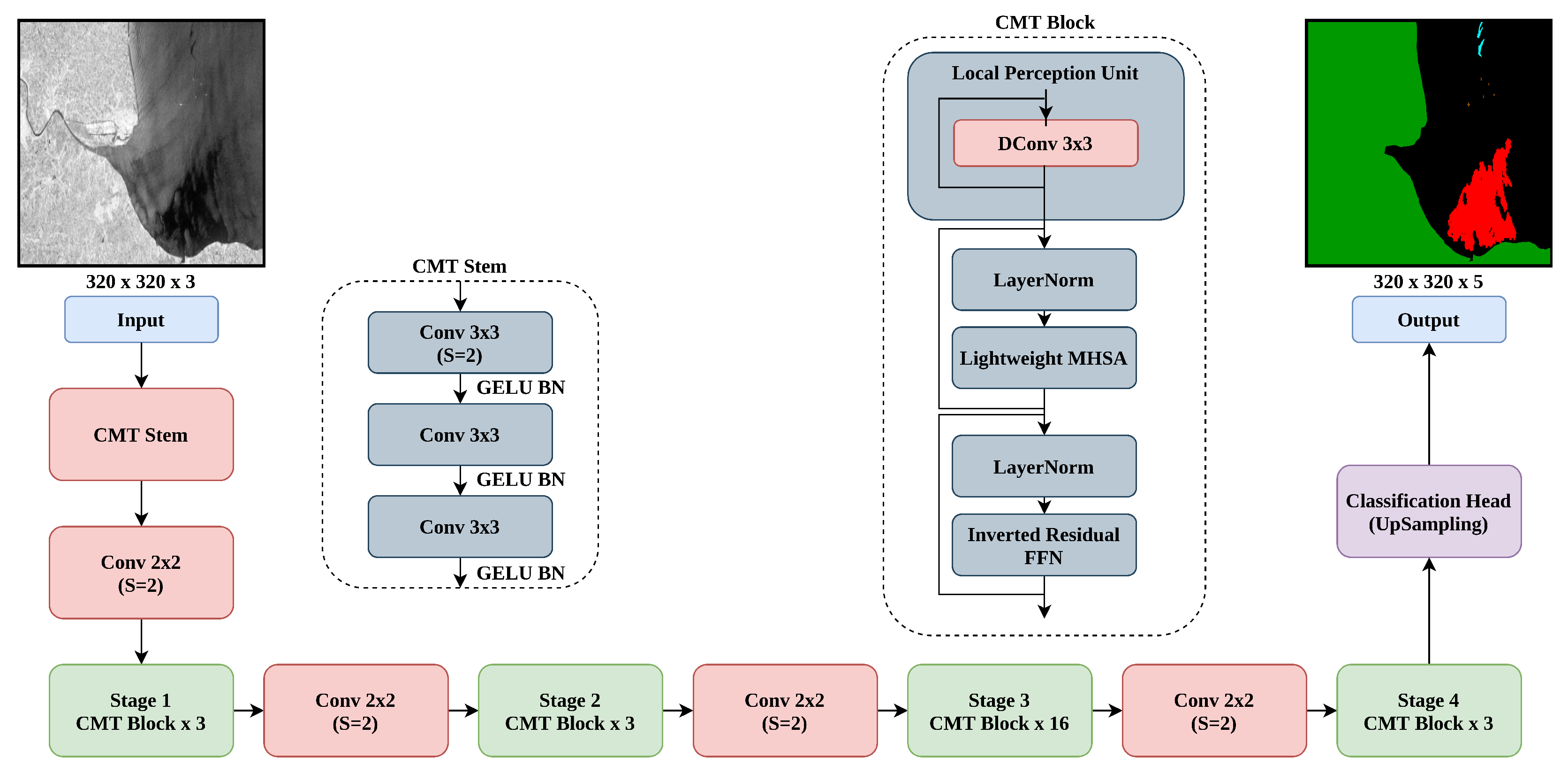
3.3. Convolutional Neural Networks Meet Vision Transformers (CMTs)

CMTs are a new family of hybrid models proposed by Guo et al. [19]. It has a CMT stem which consists of a single 3 × 3 convolutional layer with stride 2 × 2 and two 3 × 3 convolutional layers with stride 1 × 1. The rest of the network is made of alternate 3 × 3 convolutional layers with stride 2 × 2 and CMT blocks, as shown in Figure 4. Each CMT block consists of a local perception unit (LPU), lightweight multi-head self-attention (LMHSA) module, and an inverted residual feed-forward network (IRFFN). LPU extracts the local information and is defined as follows:
LPU ( X ) = DWConv ( X ) + X
where X R H × W × d , H × W represents the dimensions of the input image at current stage, and d represents the dimensions of the features. DWConv(.) is depthwise convolution. For details about LMHSA and IRFNN modules, the readers are referred to [19]. Combining the aforementioned modules, the CMT block can be defined as follows:
X i = LPU ( X i 1 ) , X i = LMHSA ( LN ( X i ) ) + X i , X i = IRFNN ( LN ( X i ) ) + X i .
where X i and X i are outputs from the LPU and LHMSA modules for block i, respectively. LN(.) represents layer normalization. We implement different variants of CMTs, viz., convolutional neural networks meet vision transformer (CMT) tiny, CMTExtraSmall, and CMTSmall, and add a classification head at the end of each architecture for semantic segmentation of SAR images. The classification head upsamples the features extracted by each CMT architecture and maps the high-level features to output, which is a semantic segmentation mask containing five classes of interest, i.e., sea surface, oil spill, lookalikes, ship, and land.

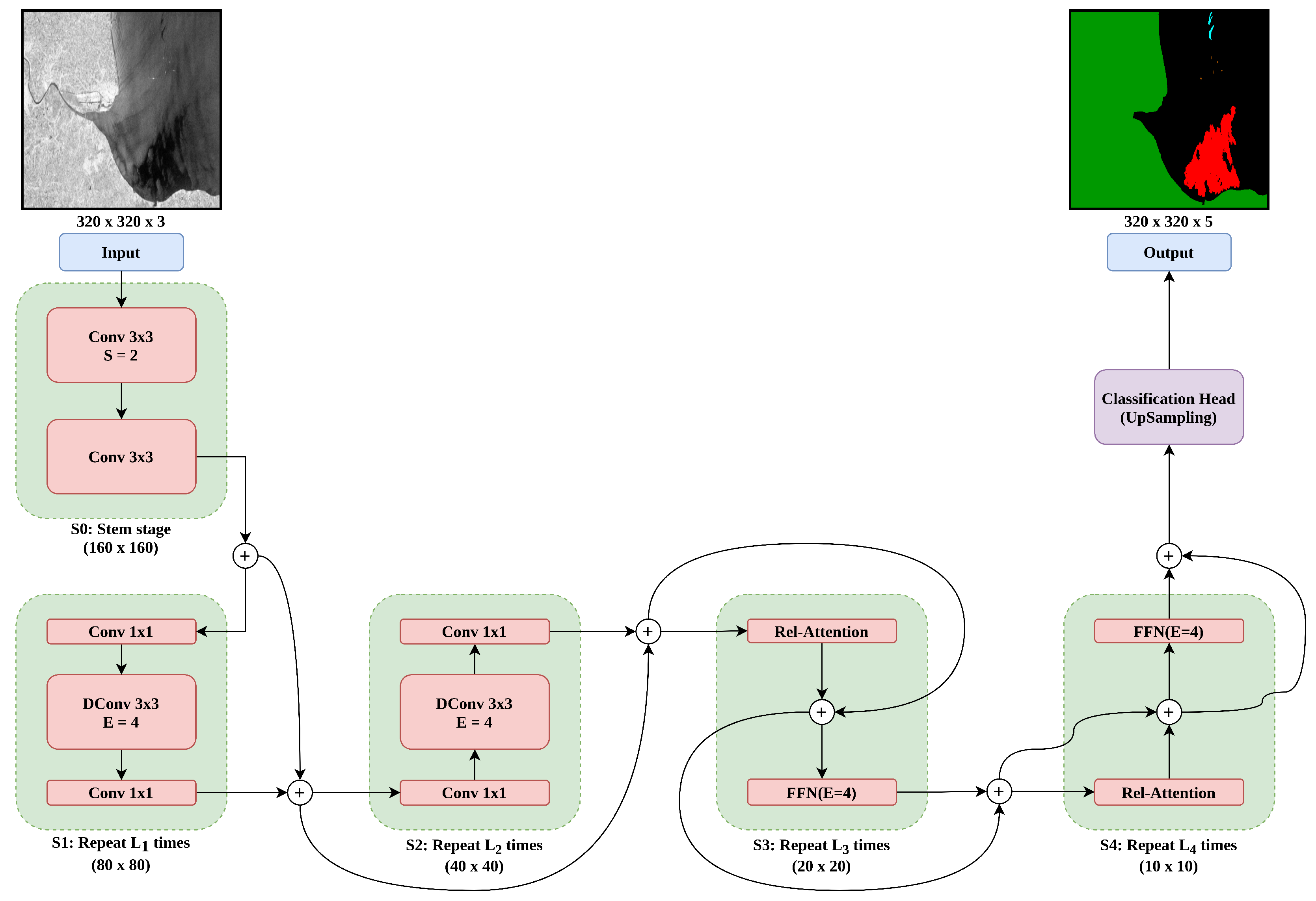
3.4. Convolution and Self-Attention Networks (CoAtNets)

CoAtNets are a family of hybrid models, recently proposed by authors in [20]. CoAtNets are built with two key insights which are as follows:
  • The advantages of both depthwise convolution and self-attention can be achieved by unifying them using simple relative attention.
  • Vertical stacking of convolution and attention layers can improve the generalization, efficiency, and capacity of the models.
The CoAtNet models are composed of five stages, i.e., S0–S4, as shown in Figure 5. The first stage consists of two 3 × 3 convolutional layers with stride 2 × 2 and 1 × 1, respectively. The second and third stages perform downsampling with depthwise convolution. Each stage consist of two 1 × 1 convolutional layers and one 3 × 3 depthwise convolution layer. The fourth and fifth stages consist of relative attention and feed-forward network (FFN) modules. For details about relative attention and FFN modules, the readers are referred to [20]. We implement the CoAtNet-0 variant of this family and add a classification head to upsample the low-level features and map the high-level features to the output, which is a semantic segmentation mask containing all the relevant classes, i.e., five in our case.

3.5. Experimental Setup

We implement the UNet CNN with different encoder backbones from the resnet series to extract complex low-level features. These features are then upsampled by simple decoder module of UNet CNN. Moreover, we implement the EfficientNetV2 family of CNNs, CMTs, and CoAtNet families of hybrid models. Apart from UNet CNN, we add a classification head to each architecture for upsampling the complex low-level features, and map the high-level features to output for semantic segmentation of SAR images. All the models are trained on the benchmark dataset introduced in Section 2. The models are trained with imagenet pretrained weights for an input shape of 320 × 320 with batch size of 12. A stochastic optimization method, namely Adam, is used. This is an efficient method for stochastic optimization with low memory requirements [43]. We are applying data augmentation on the fly. Random data augmentation generally improves the performance in various computer vision and remote sensing applications [44]. More specifically, we apply a series of random transformations including zoom range, width shift range, and height shift range of 0.3, rotation of 90°, and random vertical and horizontal flips. These random transformations are applied to SAR images as well as the ground truth masks during the training phase.

3.6. Commonly Used Semantic Segmentation Loss Functions

This subsection briefly discusses the different loss functions used for training the semantic segmentation networks.

3.6.1. Categorical Cross-Entropy Loss

The cross entropy is a measure of the difference between two probability distributions. Considering the case of binary classification, the cross-entropy loss is expressed as follows [45]:    
L CE y , p = log p , y = 1 log 1 p , otherwise .
where y { ± 1 } is the ground truth class and p [ 0 , 1 ] is the probability of predicted true class, respectively. In the context of multi-class classifications, this loss is referred to as the categorical cross-entropy loss. It measures the performance of a classification model by comparing probability distributions of ground truths and predicted class labels. If we define a new variable p t :
p t = p , y = 1 1 p , otherwise . ,
then Equation (3) can be rewritten as CE ( p t ) = log ( p t ) .

3.6.2. Categorical Focal Loss

This loss function helps in addressing the data imbalance problem. The hard examples tend to increase the classification error. Training a CNN with categorical focal loss encourages the model to pay more attention to these examples, resulting in improved classification performance. It prevents a large number of false negatives from saturating the CNN during the training phase. Mathematically, the focal loss is defined by adding the modulating factor ( 1 p t ) γ to the cross-entropy loss [45]:
L FL ( p t ) = α t ( 1 p t ) γ log ( p t )
where α and γ are the hyperparameters of focal loss.

3.6.3. Jaccard Loss

Jaccard index is one of the most commonly used metrics for semantic-segmentation-based classification problems. It measures the similarity between ground truth mask and predicted class labels. Considering y to be the ground truth mask and y ^ as the predicted class labels, the Jaccard loss function can be computed as follows [46]:
L jac ( y , y ^ ) = 1 ( y . y ^ ) + ϵ ( y + y ^ y . y ^ ) + ϵ
where ϵ is used to prevent division by zero. The subtrahend is equivalent to the intersection over union (IoU) value. Therefore, the use of Jaccard loss for the training aims to directly increase the IoU (which itself is a commonly used figure of merit for classification performance).

3.7. Gradient Profile Loss

Common cross-entropy-based losses used in semantic segmentation focus on classifying each pixel individually and do not take into account the spatial relationship over semantically constant regions. To some extent, the use of IoU-based loss (Jaccard) caters for this since it tries to increase the intersection over union of final predictions over a region. In order to illustrate this point, Figure 6 shows three images, i.e., source A (left), target B (center), and C (right). The targets B and C have the same number of white pixels but their spatial structure is different. First, we compute the mean absolute difference ( D p i x e l ) between source A and each of the target B and C by considering each pixel independently. As a result, we obtain the same value of 0.3750 for both targets. This method does not capture the different spatial patterns of target B and C. Towards this end, the complex spatial patterns in an image can be better captured by considering pixel variations along a given direction. To demonstrate this, we consider the columns of an image as vectors and compute the Euclidean distance between source A and each of the targets B and C. The mean of these distances ( D G P ) between A and B is 10.9545. Similarly, the mean of distances between A and C is 6.7082. By considering columns or rows of an image as spatial profiles, we can accurately capture the complex spatial patterns.
D p i x e l ( A , B ) = 0.3750 , D p i x e l ( A , C ) = 0.3750 , D G P ( A , B ) = 10.9545 , D G P ( A , C ) = 6.7082 .
With this motivation, we introduce the use of an additional loss that is computed in a way which preserves the spatial structure of the target label map over the entire image, in contrast to over regions or pixels. This is achieved by matching prediction probabilities along horizontal and vertical directions in the output segmentation maps. The whole row or column, a.k.a. profile, of the output prediction map is considered as a vector and matched in vector space by computing cosine similarity. This is inspired from the recently proposed spatial profile loss (SPL) [38] for use in image translation tasks. SPL computes such similarities on different color spaces and gradient spaces of the image. Our contribution is to incorporate such a matching on prediction probabilities in a semantic segmentation task. Since we are matching probability distribution along profiles, we compute this similarity over the gradients of prediction class maps. Formally, the similarity over each image channel is measured as follows:
S ( y , y ^ ) = c 1 H t r ( y c . y ^ c τ ) + 1 W t r ( y c τ . y ^ c )
where y represents the ground truth mask of size H × W , y ^ represents the predicted class labels of the same dimension, t r ( . ) represents trace of a matrix and ( . ) τ represents transpose of a matrix, and the subscript c represents each image channel. The first and second terms compute similarity between row and column profiles of ground truth mask and the predicated class labels, respectively. We compute the loss given in Equation (8) in the image gradients’ space, and call it the gradient profile (GP) loss [38]:
L GP ( y , y ^ ) = S ( y , y ^ ) .
The image gradients for each channel of an image can be easily computed by measuring image difference between an image and its one-pixel shifted version.

4. Results

The training of UNet CNN is conducted with different backbones. In particular, we used resnet50, resnet101, and resnet152 backbones. Moreover, we provide extensive ablation results on EfficientNetV2 CNNs, CMTs, and CoAtNet hybrid models. Among the different loss functions, we used categorical focal loss and Jaccard loss, as well as the GP loss. All models were trained for 62 epochs.

4.1. Comparison against State of the Art

We evaluate the performance of the classification in terms of the IoU values. The results are compared against those from the earlier work [28] as reproduced in Table 1 (row # 1 & 2). The table provides both classwise IoU and the mIoU values. Our result (row # 4, Table 1) with resnet101 backbone offers a significant improvement in terms of mIoU, which has increased by 13.5%, as well as the classwise IoU scores for all classes. The best results reported in the earlier work are achieved for the mobilenetv2 backbone; we have also outperformed those results by a significant margin for all classes except the sea surface class. For the oil spill and lookalike classes, we improve by 10.6% and 5.47%, respectively. Moreover, we carried out an ablation study by training DeepLabv3+ and UNet with mobilenetv2 backbone and a combination of GP, Jaccard, and focal loss functions. The results (row # 3 & 5, Table 1) show an improvement with mIoU score of 75.44% and 74.84%, which accounts for a 10% and 9% improvement over state of the art for this dataset, respectively. These results emphasize the advantage of adding GP loss as an additional loss function for training different backbones.
Additionally, we compare the results of our classification framework with results from earlier works on classification of oil spills [28,31,32,34,35]. Table 2 illustrates the comparison in terms of mIoU, F 1 scores, datasets used for oil spills detection, and number of classes considered for classification. Our proposed classification framework (row # 6, Table 2) provides improved results with an mIoU score of 78.45% on the oil spill detection dataset developed by MKLab ITI-CERTH, Greece, with five classes of interest, viz., sea surface, oil spills, lookalikes, ship, and land (row # 2 & 3, Table 2). We also compare our results in terms of F 1 score against those published in [31] for the same dataset (row # 1, Table 2). We achieved an F 1 score of 82.47%, which accounts for a 2.47% improvement. This highlights the significance of our proposed methodology for multi-class classification of oil spills from lookalikes, sea surface, ship, and land. For the sake of completeness and the reader’s interest, we are stating performance metrics reported by other studies on different datasets (row # 4 & 5, Table 2) with fewer classes. A direct comparison of our results with those is not possible due to difference in dataset characteristics and number of classes.

4.2. Ablation on ResNet Series

For our ablation study, we experiment with different resnet backbones trained with different loss function combinations. The results are evaluated in terms of mIoU as well as F 1 score, as reported in Table 3. When just cross-entropy loss was used in [28] with restnet101 backbone, the mIoU achieved was merely 64.97% (row # 1, Table 1). If we use a combination of categorical focal and Jaccard loss, the mIoU score jumps to 76.52% (row # 3, Table 3). Moreover, even resnet50 with 19 million fewer trainable parameters compared to resnet101 performs better with this combination (row # 1, Table 3). Remarkably, addition of GP loss further improves the overall classification performance in terms of both mIoU and F 1 scores for each backbone in our study. Classwise results have also been improved by GP loss. For the oil spill class, in particular, GP loss improves the IoU score by nearly 3–5% in each backbone.

4.3. Ablation on EfficientNetV2

We experiment with different architectures from the EfficientNetV2 family of CNNs. The mIoU and F 1 scores are used as evaluation metrics. For EfficientNetB0 (row # 3 & 4, Table 4) with 15.7 million trainable parameters, the training with a combination of focal and Jaccard loss resulted in mIoU and F 1 scores of 64.64% and 68.61%, respectively. By adding GP loss as an additional loss function, the mIoU and F 1 scores improve to 75.27% and 79.26%, respectively. This accounts for an 11% improvement with the addition of GP loss. For EfficientNetV2Small (row # 1 & 2, Table 4), EfficientNetV2B1 (row # 5 & 6, Table 4), and EfficientNetV2B2 (row # 7 & 8, Table 4), there is an improvement of 2% in mIoU and F 1 scores with the addition of GP loss as an additional loss function along with focal and Jaccard loss functions. For EfficientNetV2B3 (row # 7 & 8, Table 4), there is a 1% improvement in mIoU and F 1 scores with the addition of GP loss for training. Nevertheless, GP loss performs well for architectures with different trainable parameters.

4.4. Ablation on CMTs

To check the effectiveness of GP loss as an additional loss function for training, we experiment with CMTs: a family of hybrid models developed by combining CNNs and ViTs. The generalization ability of CNNs and capacity of ViTs is combined for better generalization and scaling. For CMTTiny (row # 1 & 2, Table 5) with 18.0 million trainable parameters, the addition of GP loss results in significant improvement in terms of mIoU and F 1 scores. The mIoU score increases by 5% from 67.16% to 72.43%, and F 1 score increases by 6% from 70.82% to 76.10%. The training of CMTXS with 23.8 million trainable parameters without addition of GP loss (row # 3, Table 5) results in low mIoU and F 1 scores. However, with the addition of GP loss, the performance significantly improves, resulting in mIoU and F 1 scores of 72.72% and 76.78%, which accounts for 17% and 18% improvement, respectively. Therefore, GP loss proves useful for training with a small training dataset. Referring to the CMTSmall (row # 5 & 6, Table 5) with 34.6 million trainable parameters, the training without the addition of GP loss results in mIoU and F 1 scores of 41.00% and 43.43%, respectively. These are the lowest scores among all the trained models. It accounts for a smaller number of training images and trainable features. However, there is a significant improvement with the addition of GP loss for training. The mIoU and F 1 scores improved to 64.50% and 67.29%, which accounts for 23% and 24% improvement, respectively.

4.5. Ablation on CoAtNet

We experiment with the CoAtNet family of hybrid models, recently proposed by Dai et al. [20]. We train the CoAtNet-0, which is the base variant of CoAtNet series with 29.4 million trainable parameters. The training of CoAtNet-0 (row 7 & 8, Table 5) is performed using a combination of focal and Jaccard loss functions. We obtained mIoU and F 1 scores of 67.00% and 70.77%, respectively. After the addition of GP loss as an additional loss function, the mIoU and F 1 scores improved to 73.61% and 77.00%, which accounts for 6% and 7% improvement, respectively. Hence, GP loss turns out to be a promising loss function for training different CNNs and ViTs-based hybrid models.

4.6. Qualitative Results

A few selected results are shown in Figure 7 for qualitative analysis. These SAR images are tested with UNet (resnet101) CNN, trained with a combination of GP, Jaccard, and focal loss functions. Referring to the top sub-figure, the model has accurately classified oil spill, lookalikes, and land area. It has also detected a small area of lookalikes that is not labeled in the ground truth mask. As such, it is difficult to say if it is a labeling error. Nonetheless, in the computation of our performance metrics, it is attributed as an error. Referring to the middle sub-figure, the model has detected the oil spills and a nearby ship. In the bottom sub-figure, the model has accurately detected oil spill and land area, but a few lookalikes predicted by the classifier close to the land seem to be in error. As per ground truth, these dark areas are just sea surface, which may represent naturally calm water close to the land.

5. Conclusions & Outlook

This paper reports an investigation into the performance of different CNNs and hybrid (CNNs + ViTs) models for oil spill classification in SAR images, and introduces the use of a new loss function, namely, gradient profile (GP) loss, that has offered significant improvements in classification performance. The problem is set up as a multi-class classification. A potential oil spill in an image has to be classified against other possible classes: natural sea surface, land, ship, and lookalikes. A labeled dataset comprising 1112 SAR images is used, which is split into training and test data subsets comprising 1002 and 110 images, respectively. State-of-the-art results reported for this dataset are an mIoU of 65.06%, using Mobilenetv2 backbone on the DeepLabv3+ architecture. Our proposed framework relies on the UNet neural network architecture, and we show our best results with the resnet101 backbone. We have achieved an mIoU of 76.52% with this framework, while training with a combination of Jaccard and focal loss functions. We achieve a further improvement of 1.93% (an overall improvement of 13.5% over state of the art) by including the GP loss function. It explicitly takes into account spatial relationships over semantically constant regions by computing cosine similarities over horizontal and vertical spatial profiles in gradients’ space. We have also performed extensive ablation studies where only the GP loss is excluded from other loss combinations in successive experiments on three different resnet backbones, EfficientNetV2 CNNs, CMTs, and CoAtNet hybrid models. In each case, the inclusion of GP loss significantly improves classwise performance (particularly for oil spill, which is an imbalanced class) as well as the overall performance.
Nevertheless, it is noteworthy to mention that the deep learning has been performed on a rather small training set with a large class imbalance. It is probable that an increased dataset may help in furthering the scores, though decent results (with F 1 > 80 ) are achieved already. We thank the researchers who set up this dataset [28,30], and for our future work, we aim to further improve our classification scores and explore the choice of GP loss as a preferred loss function for other remote sensing applications.

Author Contributions

A.B., M.S.S. and M.A.S. conceived the experiment(s). A.B. conducted the experiment(s). M.K.B. supported the empirical analysis. All authors analyzed the results. All authors reviewed the manuscript. All authors have read and agreed to the published version of the manuscript.

Funding

This research work is supported by the National Center of GIS and Space Applications (NCGSA), Islamabad, Pakistan via proposal RF-37-RS&GIS-18, as well as by Information Technology University of the Punjab’s (ITU) internal research funds.

Institutional Review Board Statement

Not applicable.

Informed Consent Statement

Not applicable.

Data Availability Statement

The oil spill detection dataset used in this study is developed by the Multimedia Knowledge and Social Media Analytics Laboratory (MKLab), ITI-CERTH, Greece and can be accessed through their website (https://mklab.iti.gr/results/oil-spill-detection-dataset/, accessed on 2 January 2022).

Acknowledgments

The authors would like to thank MKLab, ITI-CERTH, Greece, for providing a benchmark dataset for classification of oil spills [28,30].

Conflicts of Interest

The authors declare no conflict of interest.

References

  1. Solberg, A.H.S. Remote Sensing of Ocean Oil-Spill Pollution. Proc. IEEE 2012, 100, 2931–2945. [Google Scholar] [CrossRef]
  2. Solberg, A.; Storvik, G.; Solberg, R.; Volden, E. Automatic detection of oil spills in ERS SAR images. IEEE Trans. Geosci. Remote Sens. 1999, 37, 1916–1924. [Google Scholar] [CrossRef] [Green Version]
  3. Fingas, M.; Brown, C. Review of oil spill remote sensing. Mar. Pollut. Bull. 2014, 83, 9–23. [Google Scholar] [CrossRef] [PubMed] [Green Version]
  4. Zhang, L.; Zhang, L.; Du, B. Deep Learning for Remote Sensing Data: A Technical Tutorial on the State of the Art. IEEE Geosci. Remote Sens. Mag. 2016, 4, 22–40. [Google Scholar] [CrossRef]
  5. Chen, Y.; Li, Y.; Wang, J. An End-to-End Oil-Spill Monitoring Method for Multisensory Satellite Images Based on Deep Semantic Segmentation. Sensors 2020, 20, 725. [Google Scholar] [CrossRef] [Green Version]
  6. Liu, Y.; Wang, L.; Zhao, L.; Yu, Z. (Eds.) Advances in Natural Computation, Fuzzy Systems and Knowledge Discovery; Springer International Publishing: Berlin/Heidelberg, Germany, 2020. [Google Scholar] [CrossRef]
  7. Ronneberger, O.; Fischer, P.; Brox, T. U-Net: Convolutional Networks for Biomedical Image Segmentation. In Medical Image Computing and Computer-Assisted Intervention—MICCAI 2015; Springer International Publishing: Berlin/Heidelberg, Germany, 2015; pp. 234–241. [Google Scholar] [CrossRef] [Green Version]
  8. Ghosh, A.; Ehrlich, M.; Shah, S.; Davis, L.S.; Chellappa, R. Stacked U-Nets for Ground Material Segmentation in Remote Sensing Imagery. In Proceedings of the IEEE Conference on Computer Vision and Pattern Recognition (CVPR) Workshops, Salt Lake City, UT, USA, 18–22 June 2018. [Google Scholar]
  9. Li, R.; Liu, W.; Yang, L.; Sun, S.; Hu, W.; Zhang, F.; Li, W. DeepUNet: A Deep Fully Convolutional Network for Pixel-Level Sea-Land Segmentation. IEEE J. Sel. Top. Appl. Earth Obs. Remote Sens. 2018, 11, 3954–3962. [Google Scholar] [CrossRef] [Green Version]
  10. Bianchi, F.M.; Grahn, J.; Eckerstorfer, M.; Malnes, E.; Vickers, H. Snow Avalanche Segmentation in SAR Images With Fully Convolutional Neural Networks. IEEE J. Sel. Top. Appl. Earth Obs. Remote Sens. 2021, 14, 75–82. [Google Scholar] [CrossRef]
  11. Chen, L.C.; Papandreou, G.; Kokkinos, I.; Murphy, K.; Yuille, A.L. DeepLab: Semantic Image Segmentation with Deep Convolutional Nets, Atrous Convolution, and Fully Connected CRFs. IEEE Trans. Pattern Anal. Mach. Intell. 2018, 40, 834–848. [Google Scholar] [CrossRef] [Green Version]
  12. Tan, M.; Le, Q.V. EfficientNetV2: Smaller Models and Faster Training. In Proceedings of the 2021 International Conference on Machine Learning, Virtual, 18–24 July 2021. [Google Scholar]
  13. Vaswani, A.; Shazeer, N.; Parmar, N.; Uszkoreit, J.; Jones, L.; Gomez, A.N.; Kaiser, L.U.; Polosukhin, I. Attention is All you Need. In Proceedings of the Advances in Neural Information Processing Systems, Long Beach, CA, USA, 4–9 December 2017. [Google Scholar]
  14. Devlin, J.; Chang, M.W.; Lee, K.; Toutanova, K. BERT: Pre-training of Deep Bidirectional Transformers for Language Understanding. arXiv 2018, arXiv:1810.04805. [Google Scholar]
  15. Brown, T.; Mann, B.; Ryder, N.; Subbiah, M.; Kaplan, J.D.; Dhariwal, P.; Neelakantan, A.; Shyam, P.; Sastry, G.; Askell, A.; et al. Language Models are Few-Shot Learners. Adv. Neural Inf. Process. Syst. 2020, 33, 1877–1901. [Google Scholar]
  16. Wang, X.; Girshick, R.; Gupta, A.; He, K. Non-local Neural Networks. In Proceedings of the 2018 IEEE/CVF Conference on Computer Vision and Pattern Recognition, Salt Lake City, UT, USA, 18–22 June 2018; pp. 7794–7803. [Google Scholar] [CrossRef] [Green Version]
  17. Bello, I.; Zoph, B.; Le, Q.; Vaswani, A.; Shlens, J. Attention Augmented Convolutional Networks. In Proceedings of the 2019 IEEE/CVF International Conference on Computer Vision (ICCV), Seol, Korea, 27 October–2 November 2019; pp. 3286–3295. [Google Scholar] [CrossRef] [Green Version]
  18. Zhuoran, S.; Mingyuan, Z.; Haiyu, Z.; Shuai, Y.; Hongsheng, L. Efficient Attention: Attention with Linear Complexities. In Proceedings of the 2021 IEEE Winter Conference on Applications of Computer Vision (WACV), Virtual, 5–9 January 2021. [Google Scholar] [CrossRef]
  19. Guo, J.; Han, K.; Wu, H.; Xu, C.; Tang, Y.; Xu, C.; Wang, Y. CMT: Convolutional Neural Networks Meet Vision Transformers. arXiv 2021, arXiv:2107.06263. [Google Scholar]
  20. Dai, Z.; Liu, H.; Le, Q.V.; Tan, M. CoAtNet: Marrying Convolution and Attention for All Data Sizes. arXiv 2021, arXiv:2106.04803. [Google Scholar]
  21. Goodfellow, I.; Bengio, Y.; Courville, A. Deep Learning; MIT Press: Cambridge, MA, USA, 2016; Available online: http://www.deeplearningbook.org (accessed on 5 October 2021).
  22. Topouzelis, K.; Karathanassi, V.; Pavlakis, P.; Rokos, D. Detection and discrimination between oil spills and look-alike phenomena through neural networks. ISPRS J. Photogramm. Remote Sens. 2007, 62, 264–270. [Google Scholar] [CrossRef]
  23. Singha, S.; Bellerby, T.J.; Trieschmann, O. Satellite Oil Spill Detection Using Artificial Neural Networks. IEEE J. Sel. Top. Appl. Earth Obs. Remote Sens. 2013, 6, 2355–2363. [Google Scholar] [CrossRef]
  24. Garcia-Pineda, O.; MacDonald, I.R.; Li, X.; Jackson, C.R.; Pichel, W.G. Oil Spill Mapping and Measurement in the Gulf of Mexico With Textural Classifier Neural Network Algorithm (TCNNA). IEEE J. Sel. Top. Appl. Earth Obs. Remote Sens. 2013, 6, 2517–2525. [Google Scholar] [CrossRef]
  25. Guo, H.; Wei, G.; An, J. Dark Spot Detection in SAR Images of Oil Spill Using Segnet. Appl. Sci. 2018, 8, 2670. [Google Scholar] [CrossRef] [Green Version]
  26. Badrinarayanan, V.; Kendall, A.; Cipolla, R. SegNet: A Deep Convolutional Encoder-Decoder Architecture for Image Segmentation. IEEE Trans. Pattern Anal. Mach. Intell. 2017, 39, 2481–2495. [Google Scholar] [CrossRef]
  27. Orfanidis, G.; Ioannidis, K.; Avgerinakis, K.; Vrochidis, S.; Kompatsiaris, I. A Deep Neural Network for Oil Spill Semantic Segmentation in SAR Images. In Proceedings of the 2018 25th IEEE International Conference on Image Processing (ICIP), Athens, Greece, 7–10 October 2018. [Google Scholar] [CrossRef] [Green Version]
  28. Krestenitis, M.; Orfanidis, G.; Ioannidis, K.; Avgerinakis, K.; Vrochidis, S.; Kompatsiaris, I. Oil Spill Identification from Satellite Images Using Deep Neural Networks. Remote Sens. 2019, 11, 1762. [Google Scholar] [CrossRef] [Green Version]
  29. Yekeen, S.T.; Balogun, A.L.; Yusof, K.B.W. A novel deep learning instance segmentation model for automated marine oil spill detection. ISPRS J. Photogramm. Remote Sens. 2020, 167, 190–200. [Google Scholar] [CrossRef]
  30. Krestenitis, M.; Orfanidis, G.; Ioannidis, K.; Avgerinakis, K.; Vrochidis, S.; Kompatsiaris, I. Early Identification of Oil Spills in Satellite Images Using Deep CNNs. In MultiMedia Modeling; Springer International Publishing: Berlin, Germany, 2018; pp. 424–435. [Google Scholar] [CrossRef] [Green Version]
  31. Shaban, M.; Salim, R.; Khalifeh, H.A.; Khelifi, A.; Shalaby, A.; El-Mashad, S.; Mahmoud, A.; Ghazal, M.; El-Baz, A. A Deep-Learning Framework for the Detection of Oil Spills from SAR Data. Sensors 2021, 21, 2351. [Google Scholar] [CrossRef]
  32. Fan, Y.; Rui, X.; Zhang, G.; Yu, T.; Xu, X.; Poslad, S. Feature Merged Network for Oil Spill Detection Using SAR Images. Remote Sens. 2021, 13, 3174. [Google Scholar] [CrossRef]
  33. Basit, A.; Siddique, M.A.; Sarfraz, M.S. Deep Learning Based Oil Spill Classification Using Unet Convolutional Neural Network. In Proceedings of the 2021 IEEE International Geoscience and Remote Sensing Symposium IGARSS, Brussels, Belgium, 11–16 July 2021. [Google Scholar] [CrossRef]
  34. Nieto-Hidalgo, M.; Gallego, A.J.; Gil, P.; Pertusa, A. Two-Stage Convolutional Neural Network for Ship and Spill Detection Using SLAR Images. IEEE Trans. Geosci. Remote Sens. 2018, 56, 5217–5230. [Google Scholar] [CrossRef] [Green Version]
  35. Zeng, K.; Wang, Y. A Deep Convolutional Neural Network for Oil Spill Detection from Spaceborne SAR Images. Remote Sens. 2020, 12, 1015. [Google Scholar] [CrossRef] [Green Version]
  36. Kervadec, H.; Bouchtiba, J.; Desrosiers, C.; Granger, E.; Dolz, J.; Ayed, I.B. Boundary loss for highly unbalanced segmentation. Med. Image Anal. 2021, 67, 101851. [Google Scholar] [CrossRef] [PubMed]
  37. Shelhamer, E.; Long, J.; Darrell, T. Fully Convolutional Networks for Semantic Segmentation. IEEE Trans. Pattern Anal. Mach. Intell. 2017, 39, 640–651. [Google Scholar] [CrossRef]
  38. Sarfraz, M.S.; Seibold, C.; Khalid, H.; Stiefelhagen, R. Content and Colour Distillation for Learning Image Translations with the Spatial Profile Loss. arXiv 2019, arXiv:1908.00274. [Google Scholar]
  39. Konik, M.; Bradtke, K. Object-oriented approach to oil spill detection using ENVISAT ASAR images. ISPRS J. Photogramm. Remote Sens. 2016, 118, 37–52. [Google Scholar] [CrossRef]
  40. Topouzelis, K.; Psyllos, A. Oil spill feature selection and classification using decision tree forest on SAR image data. ISPRS J. Photogramm. Remote Sens. 2012, 68, 135–143. [Google Scholar] [CrossRef]
  41. Karpathy, A.; Fei-Fei, L. Deep Visual-Semantic Alignments for Generating Image Descriptions. IEEE Trans. Pattern Anal. Mach. Intell. 2017, 39, 664–676. [Google Scholar] [CrossRef] [Green Version]
  42. Vinyals, O.; Toshev, A.; Bengio, S.; Erhan, D. Show and Tell: A Neural Image Caption Generator. In Proceedings of the IEEE Conference on Computer Vision and Pattern Recognition (CVPR), Boston, MA, USA, 7–12 June 2015. [Google Scholar]
  43. Kingma, D.P.; Ba, J. Adam: A Method for Stochastic Optimization. arXiv 2015, arXiv:1412.6980. [Google Scholar]
  44. Ding, J.; Chen, B.; Liu, H.; Huang, M. Convolutional Neural Network With Data Augmentation for SAR Target Recognition. IEEE Geosci. Remote Sens. Lett. 2016, 13, 364–368. [Google Scholar] [CrossRef]
  45. Lin, T.Y.; Goyal, P.; Girshick, R.; He, K.; Dollar, P. Focal Loss for Dense Object Detection. IEEE Trans. Pattern Anal. Mach. Intell. 2020, 42, 318–327. [Google Scholar] [CrossRef] [PubMed] [Green Version]
  46. Duque-Arias, D.; Velasco-Forero, S.; Deschaud, J.E.; Goulette, F.; Serna, A.; Decencière, E.; Marcotegui, B. On power Jaccard losses for semantic segmentation. In Proceedings of the VISAPP 2021: 16th International Conference on Computer Vision Theory and Applications, Virtual, 8–10 February 2021. [Google Scholar]
Figure 1. Training dataset: A sample of two Sentinel 1 SAR images (left) along with ground truth masks (right) and class labels, viz., sea surface (black), oil spill (cyan), lookalikes (red), ship (brown), and land (green). The dataset was prepared by Krestenitis et al. [22] from the MKLab ITI-CERTH, Greece. It comprises validated oil spill records from European Maritime Safety Agency (EMSA).
Remotesensing 14 02085 g001
Figure 2. UNet architecture proposed by Ronneberger et al. [7]. It consists of an encoder part that extracts the complex low-level features by reducing the image dimensions and increasing the number of channels. The decoder part upsamples the low-level features and maps the high-level features to output, which is a semantic segmentation mask containing the desired number of classes, i.e., five in our case.
Remotesensing 14 02085 g002
Figure 3. MBConv and fused-MBConv blocks extensively utilized by EfficientNetV2 CNNs. Fused-MBConv blocks are recently proposed for better utilization of mobile or server accelerators. This replaces depthwise and expansion convolutional layers in MBConv with a single regular convolutional layer. Replacing MBConv with fused-MBConv can improve model training speed with small memory overhead.
Remotesensing 14 02085 g003
Figure 4. An overview of the CMT architecture used for semantic segmentation of SAR images for oil spill classification. The architecture is based on two modules, viz., CMT stem and CMT block. Each CMT block consists of LPU, LHMSA, and IRFNN modules. For our classification problem, the input is a 320 × 320 × 3 SAR image and output is a 320 × 320 × 5 semantic segmentation mask with five desired classes.
Remotesensing 14 02085 g004
Figure 5. An overview of the CoAtNet architecture used for semantic segmentation of SAR images for oil spill classification. It has five stages, viz., S0, S1, S2, S3, and S4. Each stage reduces the dimensions of the input image by a factor of 1/2. For our classification problem, the input is a 320 × 320 × 3 SAR image and output is a 320 × 320 × 5 semantic segmentation mask with five desired classes.
Remotesensing 14 02085 g005
Figure 6. Graphical demonstration showing importance of complex spatial patterns in different images with the same number of pixels. We compute mean absolute difference between source A (left) and each of the targets B (center) and C (right). Targets B and C have the same number of white pixels, which results in the same value of mean absolute difference. Complex spatial patterns can be captured by considering rows or columns of an image as spatial profiles.
Remotesensing 14 02085 g006
Figure 7. SAR images (left) along with ground truth masks (center) and predicted class labels (right). The classification framework used is based on UNet architecture with resnet101 pretrained encoder backbone, trained with a combination of focal, Jaccard, and GP loss functions. The images are acquired by Sentinel 1, and the training/test dataset is developed by MKLab ITI-CERTH, Greece.
Remotesensing 14 02085 g007
Table 1. Comparison of classification results with the state of the art (as reported by the earlier work [28]) assessed over the test SAR images in terms of the intersection over union (IoU) score.
RowModelBackboneLoss FunctionsTrainable
Parameters
Sea
Surface
Oil SpillLook-AlikeShipLandmIoU
1UNetResnet101Cross entropy51.5 M93.90%53.79%39.55%44.93%92.68%64.97%
2DeepLab
v3+
Mobilenetv2Cross entropy2.1 M96.43%53.38%55.40%27.63%92.44%65.06%
3DeepLab
v3+
Mobilenetv2GP + Jaccard +
focal
2.1 M96.00%53.84%59.34%70.73%97.29%75.44%
4UNetResnet101GP +Jaccard +
focal
51.5 M96.00%63.95%60.87%74.61%96.81%78.45%
5UNetMobilenetv2GP + Jaccard +
focal
10.6 M95.72%59.07%54.38%73.56%91.48%74.84%
Table 2. Comparison of the proposed classification framework with state-of-the-art classification methods based on SAR images in terms of the SAR datasets, number of classes, mIoU, and F 1 scores.
RowRelated WorkmIoU Score F 1 ScoreOil Spill DatasetNumber of Classes
1Shaban et al. [31]-80.00%MKLab ITI-CERTH, Greece.2: Oil spills and lookalikes.
2Fan et al. [32]61.90%-MKLab ITI-CERTH, Greece.5: Sea surface, oil spills,
lookalikes, ship and land.
3Krestenitis et al. [28]65.06%-MKLab ITI-CERTH, Greece.5: Sea surface, oil spills,
lookalikes, ship and land.
4Hidalgo et al. [34]-71.00%Spanish Maritime Safety and Rescue Agency
(SASEMAR).
3: Oil spills, ship and
land.
5Zeng et al. [35]-84.59%ORSI, Ocean University of China.2: Oil spills and lookalikes.
6Proposed methodology78.45%82.47%MKLab ITI-CERTH, Greece.5: Sea surface, oil spills,
lookalikes, ship and land.
Table 3. Ablation on different resnet backbones and different loss functions, evaluated over the test SAR images in terms of the IoU and F 1 scores.
RowUNet
Backbone
Loss FunctionsTrainable
Parameters
Sea SurfaceOil SpillLook-AlikeShipLandmIoU F 1 Score
1Resnet50Jaccard + focal32.5 M95.28%59.51%61.18%71.88%95.17%76.60%80.83%
2Resnet50GP + Jaccard +
focal
32.5 M95.71%62.76%59.50%72.08%97.50%77.51%81.50%
3Resnet101Jaccard + focal51.5 M95.19%58.85%60.93%73.07%94.54%76.52%80.42%
4Resnet101GP + Jaccard +
focal
51.5 M96%63.95%60.87%74.61%96.81%78.45%82.47%
5Resnet152Jaccard + focal67.1 M95.04%58.35%54.64%71.96%98.02%75.60%79.49%
6Resnet152GP + Jaccard +
focal
67.1 M95.98%62.10%62.05%72.87%97.66%78.13%82.03%
Table 4. Ablation on different variants of EfficientNetV2 CNNs and different loss functions, evaluated over the test SAR images in terms of the IoU and F 1 scores.
RowModelLoss FunctionsTrainable
Parameters
Sea SurfaceOil SpillLook-AlikeShipLandmIoU F 1 Score
1SmallJaccard + focal30.0 M95.39%51.81%59.86%69.09%95.95%74.42%78.02%
2SmallGP + Jaccard +
focal
30.0 M94.91%55.10%61.17%73.81%97.01%76.40%80.36%
3B0Jaccard + focal15.7 M94.45%50.63%63.32%23.82%90.96%64.64%68.61%
4B0GP + Jaccard +
focal
15.7 M95.09%54.03%60.40%70.47%96.38%75.27%79.26%
5B1Jaccard + focal16.7 M94.97%51.98%62.00%69.09%95.33%74.67%78.39%
6B1GP + Jaccard +
focal
16.7 M95.19%56.42%62.23%72.80%96.59%76.65%80.85%
7B2Jaccard + focal19.2 M94.91%52.16%61.88%69.09%95.64%74.74%78.59%
8B2GP + Jaccard +
focal
19.2 M95.32%55.40%61.75%70.95%96.85%76.05%80.08%
9B3Jaccard + focal24.1 M94.79%51.67%59.53%71.18%95.78%74.59%78.73%
10B3GP + Jaccard +
focal
24.1 M94.69%53.91%62.12%69.09%96.62%75.29%79.06%
Table 5. Ablation on different CNNs and ViTs-based hybrid models and different loss functions, evaluated over the test SAR images in terms of the IoU and F 1 scores.
RowModelLoss FunctionsTrainable
Parameters
Sea SurfaceOil SpillLook-AlikeShipLandmIoU F 1 Score
1CMTTinyJaccard + focal18.0 M94.98%43.57%59.95%46.01%91.30%67.16%70.82%
2CMTTinyGP + Jaccard +
focal
18.0 M94.71%50.06%57.54%69.09%90.77%72.43%76.10%
3CMTXSJaccard + focal23.8 M93.11%26.66%54.47%13.23%89.49%55.39%58.39%
4CMTXSGP + Jaccard +
focal
23.8 M95.50%51.40%58.95%64.49%93.27%72.72%76.78%
5CMTSmallJaccard + focal34.6 M90.15%12.86%40.16%16.73%45.07%41.00%43.43%
6CMTSmallGP + Jaccard +
focal
34.6 M95.02%33.14%56.98%69.09%68.26%64.50%67.29%
7CoAtNet-0Jaccard + focal29.4 M92.53%41.03%55.02%54.22%92.20%67.00%70.77%
8CoAtNet-0GP + Jaccard +
focal
29.4 M95.40%50.22%58.85%69.09%94.49%73.61%77.00%
Publisher’s Note: MDPI stays neutral with regard to jurisdictional claims in published maps and institutional affiliations.

