Article

Hybrid Network Model: TransConvNet for Oriented Object Detection in Remote Sensing Images

1
Aviation Engineering School, Air Force Engineering University, Xi’an 710038, China
2
Unbanned System Research Institute, Northwestern Polytechnical University, Xi’an 710072, China
3
National Engineering Laboratory for Wireless Security, Xi’an University of Posts and Telecommunications, Xi’an 710121, China
*
Author to whom correspondence should be addressed.
Remote Sens. 2022, 14(9), 2090; https://doi.org/10.3390/rs14092090
Submission received: 9 March 2022 / Revised: 21 April 2022 / Accepted: 21 April 2022 / Published: 27 April 2022

Abstract

:
The complexity of backgrounds, the diversity of object scale and orientation, and the defects of convolutional neural network (CNN) have always been the challenges of oriented object detection in remote sensing images (RSIs). This paper designs a hybrid network model to meet these challenges and further improve the effect of oriented object detection. The inductive bias of CNN makes the network translation invariant, but it is difficult to adapt to RSIs with arbitrary object direction. Therefore, this paper designs a hybrid network, TransConvNet, which integrates the advantages of CNN and self-attention-based network, pays more attention to the aggregation of global and local information, makes up for the lack of rotation invariability of CNN with strong contextual attention, and adapts to the arbitrariness of the object direction of RSIs. In addition, to resolve the influence of complex backgrounds and multi-scale, an adaptive feature fusion network (AFFN) is designed to improve the information representation ability of feature maps with different resolutions. Finally, the adaptive weight loss function is used to train the network to further improve the effect of object detection. Extensive experimental results on the DOTA, UCASAOD, and VEDAI data sets demonstrate the effectiveness of the proposed method.

1. Introduction

As one of the important contents of computer vision task, object detection in remote sensing images (RSIs) has broad application prospects in the fields of environmental monitoring, military investigation, national security, intelligent transportation, heritage site reconstruction, and so on.
Different from natural images, RSIs have the characteristics of variable object orientation, large scale of small object, dense object distribution, large changes in object shape, multiple scales, and complex backgrounds. According to these characteristics, many studies have proposed different improved models, and achieved good results. Yang et al. [1] improved on the basis of FasterRCNN and proposed a clustering proposal network to replace the RPN structure of the original network to capture large-scale cluster targets in aerial images. Chen et al. [2] proposed a multi-scale space and channel-aware attention mechanism to optimize the features in the backbone network of FasterRCNN [3], effectively eliminating the interference of complex backgrounds in RSIs. Wang et al. [4] designed a feature reflow pyramid network to fuse adjacent high-level features and low-level features, which effectively improved the detection effect of the detector on multi-category and multi-scale targets in RSIs. Aiming at the multi-directional targets ubiquitous in optical remote sensing images, Zhang et al. [5] improved the RPN structure in the FasterRCNN network into a rotated region proposal network and generated oriented proposals. The CADNet proposed by Zhang et al. [6] based on the FPN structure utilizes the global context mechanism and pixel-aware attention to obtain the contextual information, and introduces a space and scale-aware module to discriminate multi-scale objects, achieving high-precision detection of directional rotating objects. Yang et al. [7] proposed SCRDet and introduced the intersection over union (IoU) penalty factor to optimize the smooth L1 loss function, which effectively solved the angle period and boundary regression problems of directional target regression in RSIs. In order to realize the detection of directional remote sensing targets, Ding et al. [8] designed a region of interest transformer (RoI transformer) and carried out geometric modeling of the region of interest (RoI) through supervised learning, transitioning the detection of horizontal frame to the detection of rotating frame, and effectively aligning the features with the target frame. The detection effect is very excellent.
Although these networks have improved the performance of remote sensing image object detection effectively, these networks cannot escape the inherent properties of convolutional neural networks (CNN), which rely on two inductive biases built into the architecture itself [9]: local correlation and weight shared. When dealing with natural scene images, CNN shows good performance due to its translation invariance and focus on local information aggregation. However, in the face of RSIs with complex backgrounds, due to the lack of overall grasp of the input data and the inability to extract long-distance features between global data, the performance is not robust enough. Moreover, CNN with only a certain rotation invariance is difficult to adapt to RSIs with arbitrary object directions, thus the detection performance is not ideal. In contrast, the self-attention-based transformer [10] vision models (e.g., VIT [11] and DETR [12]) are better at dealing with information extraction of long-distance relationship due to the construction of a holistic inductive bias operator. This enables the transformer model to have a global receptive field without information loss, and pays more attention to the aggregation of global information, thereby extracting rich contextual information. When trained on large data sets, the performance of these models already rivals or even exceeds convolutional neural networks (CNN).
According to the above analysis, CNN and self-attention-based network have different defects and advantages. For object detection, the aggregation of both local and global information is useful. Therefore, based on Swin transformer [13], this paper designs a hybrid network (TransConvNet), which combines the advantages of the two models. While aggregating local information, it integrates global information to capture the interaction information between different objects and the contextual information between objects and scenes. This feature information representation is suitable for complex remote sensing images.
In addition, according to the variable scale and shape of RSIs, this paper designs an adaptive feature fusion network (AFFN). Generally, the top-level feature map has rich semantic information, but its low resolution is not enough to provide accurate location prediction. On the other hand, the low-level feature map has high resolution and contains rich detail information, but its semantic information is less, which is difficult to provide accurate semantic prediction. The classic processing method is to use feature pyramid network (FPN) [14] for feature fusion, which directly integrates the top-level feature information with the low-level feature map after upsampling. However, this method can only bring limited improvement, as the high-level feature maps still lack detailed information that is lost due to the downsampling of the backbone network. In order to overcome this defect, this paper designs AFFN structure of FPN+PAN+attention module. On the basis of FPN, path aggregation network (PAN) [15] structure is adopted to integrate the detail information of low-level into the high-level feature map. At the same time, in the FPN structure, the channel attention module [16] (CAM) is applied to reweight the feature maps in different channels to highlight the important features, in order to produce better semantic prediction. In the PAN structure, a spatial attention module [17] (SAM) is applied to focus on the locations of valid information, resulting in better location predictions. Finally, due to multi-task prediction, this paper adopts the adaptive weight loss function (AWLF) to train the network to further improve the network detection performance.
Extensive experiments are performed on the DOTA data set [18], the UCAS-AOD data set [19], and the VEDAI data set [20]. The contribution of the AFFN and AWLF to the improvement of detection performance is proved by ablation study; the experimental results compared with advanced models show that our method has the best detection effect. The main contributions of this paper are summarized as follows:
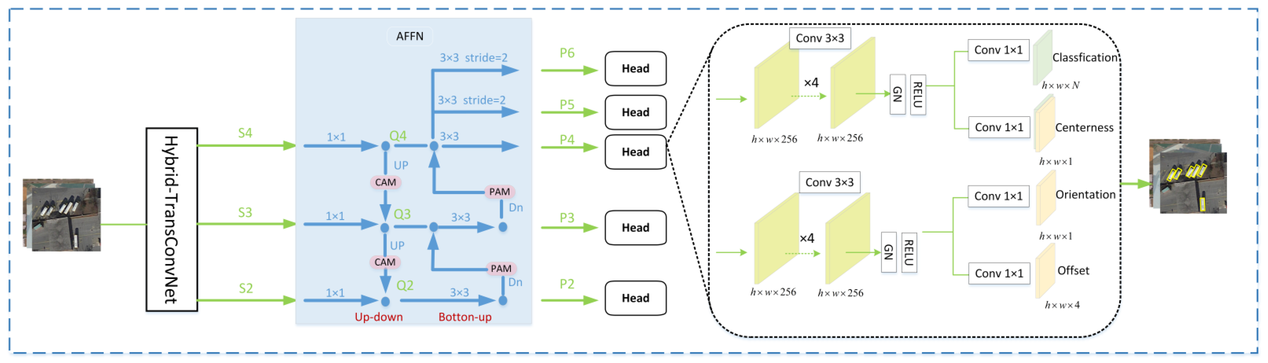
  • We design a hybrid backbone network model named TranCovNet, which improved the object detection effect of RSIs with complex background through extracted stronger feature information.
  • According to the multi-category and multi-scale characteristics of RSIs, an adaptive feature fusion network (AFFN) is proposed to make the feature maps with different resolutions in different stages contain balanced semantic information and detailed information, which improves the accuracy of detection.
  • The adaptive weight loss function (AWLF) is employed for multi task prediction to balance the loss of different tasks and better train the network.
The remainder of this article is organized as follows. The related work is briefly reviewed in Section 2. The detail of the proposed method is introduced in Section 3. In Section 4, the experimental results are reported and analyzed. Finally, the conclusion is presented in Section 5.

2. Background

2.1. Convolutional Neural Network

The strong feature extraction ability of CNN makes it still the mainstream in the field of computer vision to select CNN as the backbone network (e.g., VGG [21], RESNET [22], Efficientnet [23], Mobilenet [24]). With the emergence of RESNET [22] network, this residual connection makes the network go deeper and greatly improves the performance of the neural network. In this paper, we also learn from this structure and propose a new network structure on this basis.

2.2. Self-Attention Based Network

The success of the self-attention-based model in machine translation and natural language processing [10] has inspired people to try to apply this idea to image recognition [11,25,26] and object detection [12,27]. The core of these models is the self-attention mechanism, which can obtain the global representation information through the calculation of self-attention. An attention function can be described as mapping a query and a set of key-value pairs to an output, where the query, key, and value are vectors from the linear mapping of the input. The output is computed as a weighted sum of the values, where the weight is assigned to each value is computed by a compatibility function of the query with the corresponding key. At present, the calculation of self-attention can be divided into scaled dot-product attention, multi-head attention, and local window attention. They can be described as follows:

2.2.1. Scaled Dot-Product Attention

Value ( V ) is weighted according to the similarity between query ( Q ) and key ( K ); Q and K of dimension d k , and V of dimension d v are obtained from the same input through linear transformation. Scaled dot-product attention is defined as follows:
A t t e n t i o n ( Q , K , V ) = s o f t max ( Q K T d k ) V

2.2.2. Multi-Head Attention

Firstly, Q , K , and V are linearly projected for h time with different, learned linear projections, respectively. Then the single head dot product attention is calculated for the values obtained each time. On each of these projected versions of Q , K , and V we then perform the attention function in parallel. These are concatenated and once again projected, resulting in the final values. The calculation process is as follows:
M u l t i H e a d ( Q , K , V ) = c o n c a t ( h e a d 1 , , h e a d h ) W O h e a d i = A t t e n t i o n ( Q W i Q , K W i K , V W i V )

2.2.3. Local Window Attention

In the standard transformer mechanism [10], the computation of global attention makes the computational complexity grow quadratically with the number of input sequence data, which is not suitable for computer vision problems that require dense predictions or high-resolution images. In the paper [13], the authors proposed self-attention in a local window to reduce the computational and storage complexity. The image is equally divided into non-overlapping windows, each window contains M × M patches, and the multi-head attention calculation is performed in each window.

2.3. Feature Fusion Network

In many deep learning tasks (such as object detection, image segmentation), fusing features of different scales is an important means to improve performance. Low-level features have higher resolution and contain more location and detail information, but they have lower semantics and more noise due to fewer convolutions. High-level features have stronger semantic information, but low resolution and poor perception of details. How to fuse them efficiently is the key to improve the segmentation model. SSD [28] and MS-CNN [29] does not fuse features, but predicts multi-scale features separately, and then integrates the prediction results. FPN [14] performs feature pyramid fusion and prediction after fusion. In order to better solve the problem caused by scale changes in object detection, M2det [30] proposes a more effective feature pyramid structure, MLFPN (multi-level feature pyramid network). For FPN-based single-stage detectors, the inconsistency between different feature scales is their main limitation. YOLOv3-ASFF [31] proposes a new data-driven pyramid feature fusion method, called adaptive spatial feature fusion (ASFF).

3. Materials and Methods

The overall framework of the detection method in this paper is presented in Figure 1. It mainly includes: TransConvNet backbone network, adaptive feature fusion network (AFFN), and multi-task prediction head. TransConvNet backbone network (as shown in Figure 2) includes four stages, in which S1, S2, S3, and S4 represent different depth feature maps extracted in the first, second, third, and fourth stages of the network, and the sizes are 1/4, 1/8, 1/16, and 1/32 of the original input image size, respectively. S2, S3, and S4 are sent into AFFN to obtain feature maps P2, P3, P4, P5, and P6 with different resolutions, which are 1/8, 1/16, 1/32, 1/64, and 1/128 of the original size, respectively. These five feature maps are sent to the detection head network to predict the object classification confidence, center confidence, angle, and distance offset, respectively. The feature maps of different sizes predict the object of different size ranges. The regression ranges of P2, P3, P4, P5, and P6 are (0, 64], (64, 128], (128, 256], (256, 512] and (512, ∞), respectively. The following is a detailed introduction to the TransConvNet backbone network (shown in Figure 2), the adaptive feature fusion network (shown in the AFFN module in Figure 1), the multi-task detector head, and the adaptive weight loss function.

3.1. TransConvNet Backbone Network

As shown in Figure 2, TransCovNet backbone network is an essential component of our method for feature extraction, which is mainly composed of Patchify Stem and four stages. Each stage contains different numbers of transformer block and conv block.

3.1.1. Patchify Stem

The main function of Patchify Stem is to convert 2D RGB image ( H × W × 3 ) into 1D sequence data. In classical papers, such as VIT [11] and Swin transformer [13], the usual approach is to first hard segment the image into non overlapping image blocks ( P × P ), and then linearly encode each image block through a linear embedding layer, project it to dimension C and convert it into 1D sequence data. In the code implementation, the convolution operation with convolution kernel size of P × P and step size of P is used. However, this kind of hard segmentation easily makes the network unable to model the local structure of the image (such as edges and lines), thus a large number of training samples are needed to obtain the similar performance of CNN.
In this paper, we adopt two convolution operations with a convolution kernel size of ( 3 × 3 ) and a stride of 2 to realize the aggregation of local features, and then connect a ( 1 × 1 ) convolution to adjust the dimension to C and realize the integration of cross-channel information. Finally, the feature of H / 4 × W / 4 × C is obtained and transformed into sequence data of ( H / 4 × W / 4 ) × C through reshape operation.

3.1.2. Transformer Block and Conv Block

Each stage of the backbone network includes two modules: transformer block and conv block.
Transformer block is shown in Figure 2a. In order to reduce the complexity of self-attention calculation, the input data is first reduced by ( 1 × 1 ) convolution to reduce the dimension. By arranging the windows, the image is evenly divided into windows of size ( M × M ) in a non-overlapping manner, the attention calculation is performed inside each window, and the ( 1 × 1 ) convolution is connected at the output to increase the dimension. The operation process in transformer block can be expressed as:
z ˜ l = W M S A [ L N ( f 1 × 1 ( z l 1 ) ) ] + f 1 × 1 ( z l 1 )
z l = f 1 × 1 [ M L P ( L N ( z ˜ l ) ) + z ˜ l ]
where z l 1 and z l are the input and output of the l -th transformer block, and W M S A is window-based self-attention calculation.
After the transformer block, the conv block is connected (shown in Figure 2b) to realize the fusion of data and the interaction of data between windows, and to model the global relationship. This attention with local and global receptive fields helps the model learn strong informative representations of images.
Each conv block consists of three convolutional layers, namely, 1 × 1, 3 × 3, and 1 × 1 filters. Downsampling is performed in the first conv block with a stride of 2. The process can be expressed as:
z ^ l + 1 = R E L U ( B N ( f 1 × 1 ( z l ) ) )
z ^ ^ l + 1 = R E L U ( B N ( f 3 × 3 ( z ^ l + 1 ) ) )
z l + 1 = R E L U ( B N ( f 1 × 1 ( z ^ ^ l + 1 ) ) + s h o r t c u t
Residual connections follow two simple design rules: (a) after the first conv block, the feature map size is halved; (b) after the second conv block, the feature map size is unchanged. The residual connections can be expressed as:
( a ) :   s h o r t c u t = B N ( f 1 × 1 ( B N ( f 3 × 3 ( z l ) ) ) )
( b ) :   s h o r t c u t = z l
where, z l and z l + 1 are the input and output of the l -th conv block.
This paper builds four kinds of models, which are TransConvNet-T, TransConvNet-S, TransConvNet-B, and TransConvNet-L, as shown in Table 1. The window size is set to M = 7 by default, the dimension of each head is d = 32 , and the expansion layer of each MLP is α = 4 , for all experiments. The architecture hyper-parameters of these model variants are:
TransConvNet-T: C = 64 , Block numbers in each stage = {(2,1),(2,2),(6,2),(2,2)}
TransConvNet-S: C = 64 , Block numbers in each stage = {(2,1),(2,2),(18,2),(2,2)}
TransConvNet-B: C = 128 , Block numbers in each stage = {(2,1),(2,2),(18,2),(2,2)}
TransConvNet-L: C = 256 , Block numbers in each stage = {(2,1),(2,2),(18,2),(2,2)}

3.2. Adaptive Feature Fusion Network

The network structure is shown in the AFFN module in Figure 1. The adaptive feature fusion network is divided into two stages. The first stage is the FPN [14] structure, which transfers the high-level semantic information to the low-level feature map from top to bottom. The second stage is the PAN [15] structure. In order to make up for the detail information lost in the backbone network due to downsampling, a bottom-up feature fusion is constructed, so that the detail location information is transferred to the deep-level feature map. In addition, channel attention and spatial attention are respectively introduced into the two fusion methods to improve the fusion effect. The final output feature maps of different scales contain strong semantic information and rich detailed information. The specific process is as follows:
The feature maps S2, S3, and S4 extracted from the backbone network are sent to the AFFN. In the FPN structure, S2, S3, and S4 carry out top-down feature fusion. First, the feature maps of each level are followed by a 1 × 1 convolutional layer to keep the number of channels consistent, and Q4 is obtained by direct convolution of S4. Then S4 is upsampled by bilinear interpolation to improve the resolution of the feature map. After the channel attention module (as shown in Figure 3), the feature maps in different channels are reweighted to emphasize important features and compress unimportant features. The recalibrated features are added and fused with S3 to obtain Q3. In the same operation, Q3 is added and fused with S2 after upsampling and channel attention module to obtain Q2.
Then enter the second stage, in the PAN structure, Q2, Q3, and Q4 perform bottom-up feature fusion. P2 is obtained directly from Q2 through a 3 × 3 convolution layer. Downsampling P2 to reduce the resolution of the feature map, focusing the position of the effective information in the feature map through the spatial attention module (as shown in Figure 4), fusion with Q3, and finally obtaining P3 after 3 × 3 convolutional operation. With the same operation, P3 is added and fused with Q4 after downsampling and spatial attention, and then P4 is obtained through a 3 × 3 convolution layer. P5 and P6 are produced by applying a convolutional layer with stride of 2 on P4.
In our method, the output feature maps P2, P3, P4, P5, and P6 of the AFFN are respectively allocated with the regression range of (0, 64], (64, 128], (128, 256], (256, 512], (512, ∞), so that small objects are detected on low-level high-resolution feature maps, and large objects are detected on high-level low-resolution feature maps. Through the adaptive feature fusion network, the feature maps with different resolutions balance semantic information and location information, which improves the recall and accuracy of object detection.

3.3. Multi-Task Detector Head

As displayed in Figure 1, the multi-task detector head has four subtasks including classification, centerness confidence, distance offset, and angle prediction.
The output P i ( i = 2 , 3 , 4 , 5 , 6 ) of AFFN is sent to the multi-scale detection head, respectively. Consistent with the setting of FCOS [32], first, the feature map F i h × w × 256   ( i = 2 , 3 , 4 , 5 , 6 ) is obtained through a 3 × 3 convolutional layer stacked four times. Then it is divided into four branches, after normalization, activation function and 1 × 1 convolutional layer, the feature maps f c l c h × w × N , f c e n t e r h × w × 1 , f θ h × w × 1 , f o f f s e t h × w × 4 are obtained. Finally, these four feature maps are used for multi-task prediction and regression, respectively, including object classification confidence prediction, center confidence prediction, angle regression, and distance offset regression.

3.3.1. Box Regression

At present, remote sensing object detection usually adopts five parameters to represent the oriented bounding box (OBB), that is ( x c , y c , w , h , θ ) , as shown in Figure 5a. Where ( x c , y c ) represents the coordinate of the center point, ( w , h ) represents the width and height of the bounding box, θ represents the angle between the horizontal axis at the lowest point of OBB and the first edge encountered by counterclockwise rotation, and the first edge contacted is the width of the object box, i.e., w .
However, this representation method will be accompanied by a typical boundary mutation problem when performing rotation box coordinate regression. Besides, our paper adopts the pixel-wise predictive regression of FCOS [32] to generate bounding boxes. Therefore, we redefine a new representation method. As shown in Figure 5b, the directional bounding box can be expressed as ( x , y , Q i , θ , ( i = 1 , 2 , 3 , 4 ) ) , where ( x , y ) represents the coordinates of a certain point in the figure, and a Cartesian coordinate system is established with this point as the origin, Q i ( i = 1 , 2 , 3 , 4 ) represents the distance offset from the point to the bounding box and is located in the i-th quadrant, and θ is the angle between the X-axis and Q 1 .
For each location ( x , y ) on the feature map f c l c h × w × N , we can map it back onto the input image as ( x s + s 2 , y s + s 2 ) , which is near the center of the receptive field of the location ( x , y ) . If the point is within a ground truth bounding box, the point is a positive sample; otherwise, it is a negative sample. If it is a positive sample, the distance from the point to the border of the ground truth and angle are regressed, and the regression target is ( Q i * , θ * ) = ( Q 1 * , Q 2 * , Q 3 * , Q 4 * , θ * ) .
Given that the coordinates of the four vertices of the ground truth box are { ( P i x , P i y ) | i = 1 , 2 , 3 , 4 } and the coordinates of a point in the box are ( a x , a y ) , the algorithm for finding Q i * is as follows (Algorithm 1):
Algorithm 1: Distance offset calculation procedure
Input:  { ( P i x , P i y ) | i = 1 , 2 , 3 , 4 } : coordinates of the four vertices of the ground truth
( a x , a y ) : coordinates of the regression point
Output: regression distance offset target Q i *
1 set P 1 x = P max x , the rest of the coordinates are arranged counterclockwise based on P 1 x
2 if  P 1 x = P 2 x or P 1 x = P 4 x  then
3   Q 1 * = P 1 x a x , Q 2 * = P 2 y a y , Q 3 * = a x P 3 x , Q 4 * = a y P 4 y
4 else
5  for  i = 1 ; i < 4 ; i + +  do
6     S i = s q r t ( ( P i x P i + 1 x ) 2 + ( P i y P i + 1 y ) 2
7     D i = s q r t ( ( P i x a x ) 2 + ( P i y a y ) 2 )
8     p i = ( D i + D i + 1 + S i ) / 2
9     s i = s q r t ( p i × ( p i S i ) × ( p i D i ) × ( p i D i + 1 ) ) (Heron’s formula)
10     Q i = 2 * s i / S i
11   return  Q i
12 end
13 end

3.3.2. Center Confidence

This paper adopts the same settings as in [32] to reduce the low-quality bounding boxes predicted by points farther from the center point. In training, it is trained as a sub-task with the cross-entropy function as the loss function. In reasoning, the product of the classification confidence and the center confidence is taken as the final score. If the score is greater than 0.05, it is taken as a positive sample. The center confidence can be expressed as:
c e n t e r n e s s * = min ( Q 1 , Q 3 ) max ( Q 1 , Q 3 ) × min ( Q 2 , Q 4 ) max ( Q 2 , Q 4 )

3.4. Adaptive Weight Loss Function

The multitask learning loss function is composed of one classification loss for classification prediction, one centerness confidence loss for centerness prediction, and two regression loss for distance offset and angle prediction. To jointly learn these four subtasks, the uncertainty weighted loss is employed to capture the relative confidence among the four subtasks.
The classification loss function adopts the focal loss function [33]. The formula is defined as follows:
L c l s = 1 N p o s x , y L c l s ( p x , y , c x , y * ) = 1 N p o s x , y { α ( 1 p x , y ) γ log ( p x , y ) c x , y * = 1 ( 1 α ) P x , y γ log ( 1 p x , y ) o t h e r w i s e
where N p o s represents the number of positive samples. p x , y and c x , y * are the predicted classification confidence and its true value at point ( x , y ) . In the experiment, α and γ are set to 0.25 and 2, respectively.
The center confidence loss function adopts the cross entropy loss function, and the calculation method is as follows:
L c e n t e r n e s s = 1 N p o s x , y { c x , y log ( c e n t e r n e s s * ) + ( 1 c x , y ) log ( 1 c e n t e r n e s s * ) }
where c x , y { 0 , 1 } represents that the point ( x , y ) is a negative sample or a positive sample. c e n t e r n e s s * [ 0 , 1 ] depicts the normalized distance from the location to the center of the object that the location is responsible for, as shown in Equation (10).
The bounding box regression loss consists of two parts, one is the distance offset loss and the other is the angle loss. They are respectively defined as follows:
L offset   =   1 N pos x , y 1 { c x , y = 1 } smooth L 1 ( t x , y t x , y * )
L orientation   =   1 N pos x , y 1 { c x , y = 1 } smooth L 1 ( θ x , y θ x , y * )
where 1 { c x , y = 1 } represents an indicator function that returns one if C x , y = 1 (i.e., positive sample) and otherwise returns zero. θ x , y and t x , y = { Q i | i = 1 , 2 , 3 , 4 } x , y indicate the predicted values of angle and offset at the point ( x , y ) , respectively. θ x , y * and t x , y * represent their true values. The smooth L1 loss can be calculated as:
S m o o t h L 1 ( x ) = { 0.5 x 2 , | x | < 1 | x | 0.5 , o t h e r w i s e
Finally, this paper uses uncertainty loss to balance these multi task losses. The specific formula is as follows:
L = 1 δ 1 2 L c l c + 1 δ 2 2 L c e n t e r n e s s + 1 2 δ 3 2 L o f f s e t + 1 2 δ 4 2 L o r i e n t a t i o n + 2 log δ 1 δ 2 δ 3 δ 4
where δ 1 , δ 2 , δ 3 , and δ 4 are learnable uncertainty weighting factors used to balance multi task loss. The specific introduction of weight uncertainty loss is detailed in reference [34].

4. Experiments and Results Analysis

In this section, three public optical remote sensing image data sets and evaluation metrics are first introduced. Then, the contribution of TransCovNet backbone, AFFN, and AWLF are analyzed. Next, the superiority of the proposed method is analyzed in comparison with the state-of-the-art detectors. Finally, some promising detection results are displayed.

4.1. Data Set and Training Details

In our experiments, we chose three oriented optical remote sensing image data sets: the DOTA [18] data set, the UCAS-AOD [19] data set, and the VEDAI [20] data set.

4.1.1. DOTA Data Set

The DOTA data set consists of 2806 remote sensing images from different sensors and platforms, ranging from 800 × 800 to 4000 × 4000 pixels, which contain 188,282 object instances with different scales, orientations, and shapes. The categories of the data set include plane, helicopter, swimming pool, roundabout, harbor, basketball court, soccer ball field, tennis court, ground track court, baseball diamond, storage tank, bridge, ship, small vehicle, and large vehicle. In this data set, the proportions of training, validation, and test images are 1/2, 1/6, and 1/3, respectively. Multiple sizes were used for the crop images; the sizes used were 512 × 512, 800 × 800, and 1024 × 1024 with 0.2 overlaps.

4.1.2. UCAS-AOD Data Set

The UCAS-AOD data set mainly contains two types of targets: plane and car. There are 1000 plane images and 520 car images, including 7482 plane targets and 7144 car targets. The target is annotated with oriented bounding boxes consisting of four vertex coordinates. In the experiment, the data are randomly divided into training set, validation set, and test set according to the ratio of 7:2:1.

4.1.3. VEDAI Data Set

The VEDAI data set is a data set for vehicle detection in aerial images, with a total of 1210 images containing 3640 vehicle objects. In this experiment, the data set is randomly divided into training set and test set according to 9:1.

4.1.4. Training Details

The experiment in this article uses the pytorch deep learning framework, uses 2 GTX 1080Ti GPUs for accelerated training, and sets the single GPU BatchSize to 4. At the same time, the Adam optimizer [35] with an initial learning rate of 1 × 10 4 is used to optimize the network. In this experiment, the DOTA data set, the UCAS-AOD data set, and the VEDAI data set were iteratively trained for 100, 120, and 140 epochs, respectively, and the optimizer learning rate decay with a decay rate of 10 was performed at the 80th, 100th, and 120th epochs.

4.2. Evaluation Metrics

To quantitatively evaluate the performance of the proposed method, we adopt five widely used evaluation metrics, namely, precision, recall, average precision, mean average precision, and F 1 s c o r e . The calculation formulas are as follows:
P r e c i s i o n = T P T P + F P
R e c a l l = T P T P + F N
where T P is the true positive, F P is the false positive, and F N is the false negative. P r e c i s i o n represents the ratio of correctly identified positive objects to detected positive samples and R e c a l l represents the ratio of correctly identified positive objects to all positive samples.
A P metric is measured by the area under the precision-recall curve, which comprehensively measures the precision and recall rate of a certain class.
A P = 0 1 P ( R ) d R
m A P can be used as an evaluation index for multi-class target detection accuracy.
m A P = 1 N c i = 1 N c 0 1 P i ( R i ) d R i
where N c represents the number of categories in the data set, and P i and R i represent the precision and recall rate of the i-th target.
F 1 can evaluate the one-class object detection performance comprehensively.
F 1 = 2 × P r e c i s i o n × R e c a l l P r e c i s i o n + R e c a l l

4.3. Backbone Network Performance Analysis

Experiments are carried out on the UCAS-AOD data set to compare the three detection methods of RoI-transformer [8], R3Det [36] and our method, using ResNet50 [22], Swin transformer-T [13] and TransConvNet-T three backbone networks, respectively, and to test their detection performance, as shown in Table 2. It can be seen that the performance of the same detection method using the backbone network of this paper has been improved to varying degrees. For the RoI-transformer detection method, the mAP value is increased by 5.24% compared with the CNN of the same level, and by 2.05% compared with the Swin-T backbone network; For R3Det, compared with the CNN at the same level, the mAP value is increased by 5.05% and 1.44% compared with Swin-T backbone network; for the detection method in this paper, the mAP value is increased by 4.95% compared with the convolutional neural backbone network of the same level, and 1.96% higher than that of the Swin-T backbone network.
Experiments are performed on the VEDAI data set. Using the adaptive feature fusion network, detection head, and loss function proposed in this paper, the performance of TransConvNet with four different capacities is tested, as shown in Table 3.

4.4. Ablation Study

The adaptive feature fusion network (AFFN) and the adaptive weight loss function (AWLS) are the two important components proposed in this paper. In order to test their contribution to the detection performance, relevant ablation experiments are carried out on the VEDAI data set. The baseline model uses TransConvNet-B as the backbone network, using FPN feature fusion strategy and equal weight loss function.
As shown in Table 4, after selecting the AFFN, the recall rate is increased by 3.44%, the accuracy rate is increased by 2.22%, and the F1 score is increased by 2.9%. After selecting the AWLF, the recall rate, precision rate, and F1 score are increased by 1.7%, 1.44%, and 1.6%, respectively. Compared with the two, the former contributes more to the improvement of recall rate and precision rate, which may benefit from the internal mechanism of the AFFN, so that the feature map evenly contains the information representation required for detection. Figure 6 shows visualization results of the baseline model after adopting an AFFN and an AWLF. The first row is the detection result of the baseline model. It can be seen that there are some missed detections and the bounding box is not accurate enough. The second row is the detection result after select the adaptive feature fusion network and it can be seen that the missed detection has improved. The third row is the detection result after selecting the adaptive weight loss function, and it can be seen that the detected bounding box is more accurate. The last row is the detection result of both the adaptive feature fusion network and the adaptive weight loss function that are used.

4.5. Comparison with State-of-the-Art Methods

To comprehensively verify the superiority of our method, we conduct comparative experiments on the DOTA data set. As shown in Table 5, we compared the AP in 15 categories and mAP value with another eight deep learning-based methods. Among them, ROI-Trans [8], CAD-Net [6], R3Det [36], SCRDet [7], GV [37], BBAVector [38], and CSL [39] adopted ResNet-101-FPN as the backbone network, except that RRPN [40] used VGG 16 as the backbone network. Note that data augmentation was applied for a fair comparison with all the compared methods. In Table 5, red and blue represent the optimal and second-best detection results, respectively. As can be seen from the table, the mAP value of the method in this paper reaches 78.41%, which is 2.24% higher than the CSL method with the best performance in the anchor-based model, and 3.05% higher than the BBAVectors method based on the anchor-free mechanism, obtained state-of-the-art performance on the DOTA data set. In addition, the detection performance on densely arranged small targets, such as small vehicles and large vehicles, has improved significantly, reaching 80.23% and 82.43% AP values, respectively, which are 1.97% and 2.03% higher than the second best. At the same time, the method in this paper achieves the optimal detection in the detection of bridges and ships, and achieves second-best detection in the detection of soccer ball fields and roundabouts. Finally, we present the visualization of the detection results for the DOTA data set in Figure 7.

5. Conclusions

In order to cope with the complexity of remote sensing image background, the diversity of target scale and orientation, and the shortcomings of convolutional neural networks, this paper proposes a new backbone network, TransCovNet, which combines the advantages of convolutional neural network and self-attention-based network to better extract the information representation of image for object detection. On this basis, this paper also proposes an adaptive feature fusion network, which makes the feature representation of different resolutions of the image contain balanced semantic information and location detail information, and further improves the accuracy of object detection, especially for the improvement of recall rate. Finally, the network is trained with the adaptive weight-loss function, which further achieves good results. We performed extensive comparisons and ablation experiments on the DOTA, UCAS-AOD, and the VEDAI data sets. The experimental results prove the effectiveness of our method for oriented object detection in remote sensing images. In future work, we will design a more lightweight and efficient backbone network to speed up the real-time performance of the detector for detecting oriented targets in optical remote sensing images.

Author Contributions

Methodology, L.H.; software, C.W.; validation, Z.C.; formal analysis, L.H.; investigation, S.M.; resources, Z.C.; data curation, S.M.; writing—original draft preparation, X.L.; writing—review and editing, X.L.; visualization, Z.C.; supervision, S.M.; project administration, C.W.; funding acquisition, L.H. All authors have read and agreed to the published version of the manuscript.

Funding

This work was supported in part by the National Natural Science Foundation of China under Grant 61701524 and in part by the China Postdoctoral Science Foundation under Grant 2019M653742 (corresponding author: L.H.).

Data Availability Statement

The data used to support the findings of this study are available from the corresponding author upon request.

Conflicts of Interest

The authors declare no conflict of interest.

References

  1. Yang, F.; Fan, H.; Chu, P.; Blasch, E.; Ling, H. Clustered object detection in aerial images. In Proceedings of the IEEE International Conference on Computer Vision, Seoul, Korea, 27–28 October 2019; pp. 8311–8320. [Google Scholar]
  2. Chen, J.; Wan, L.; Zhu, J.; Xu, G.; Deng, M. Multi-scale spatial and channel-wise attention for improving object detection in remote sensing imagery. IEEE Geosci. Remote Sens. Lett. 2019, 17, 681–685. [Google Scholar] [CrossRef]
  3. Ren, S.; He, K.; Girshick, R.; Sun, J. Faster r-cnn: Towards real-time object detection with region proposal networks. arXiv 2015, arXiv:1506.01497. [Google Scholar] [CrossRef] [PubMed] [Green Version]
  4. Wang, J.; Wang, Y.; Wu, Y.; Zhang, K.; Wang, Q. FRPNet: A feature-reflowing pyramid network for object detection of remote sensing images. IEEE Geosci. Remote Sens. Lett. 2020, 19, 8004405. [Google Scholar] [CrossRef]
  5. Zhang, Z.; Guo, W.; Zhu, S.; Yu, W. Toward arbitrary-oriented ship detection with rotated region proposal and discrimination networks. IEEE Geosci. Remote Sens. Lett. 2018, 15, 1745–1749. [Google Scholar] [CrossRef]
  6. Zhang, G.; Lu, S.; Zhang, W. Cad-net: A context-aware detection network for objects in remote sensing imagery. IEEE Trans. Geosci. Remote Sens. 2019, 57, 10015–10024. [Google Scholar] [CrossRef] [Green Version]
  7. Yang, X.; Yang, J.; Yan, J.; Zhang, Y.; Zhang, T.; Guo, Z.; Sun, X.; Fu, K. Scrdet: Towards more robust detection for small, cluttered and rotated objects. In Proceedings of the IEEE International Conference on Computer Vision, Thessaloniki, Greece, 23–25 September 2019; pp. 8232–8241. [Google Scholar]
  8. Ding, J.; Xue, N.; Long, Y.; Xia, G.S.; Lu, Q. Learning RoI transformer for oriented object detection in aerial images. In Proceedings of the IEEE Conference on Computer Vision and Pattern Recognition, Long Beach, CA, USA, 16–20 June 2019; pp. 2849–2858. [Google Scholar]
  9. D’Ascoli, S.; Touvron, H.; Leavitt, M.L.; Morcos, A.S.; Biroli, G.; Sagun, L. Convit: Improving vision transformers with soft convolutional inductive biases. In Proceedings of the International Conference on Machine Learning, PMLR, Virtual, 18–24 July 2021; pp. 2286–2296. [Google Scholar]
  10. Vaswani, A.; Shazeer, N.; Parmar, N.; Uszkoreit, J.; Jones, L.; Gomez, A.N.; Kaiser, Ł.; Polosukhin, I. Attention is all you need. Adv. Neural Inf. Process. Syst. 2017, 3, 5998–6008. [Google Scholar]
  11. Dosovitskiy, A.; Beyer, L.; Kolesnikov, A.; Weissenborn, D.; Zhai, X.; Unterthiner, T.; Dehghani, M.; Minderer, M.; Heigold, G.; Gelly, S. An image is worth 16 × 16 words: Transformers for image recognition at scale. arXiv 2020, arXiv:2010.11929. [Google Scholar]
  12. Carion, N.; Massa, F.; Synnaeve, G.; Usunier, N.; Kirillov, A.; Zagoruyko, S. End-to-end object detection with transformers. In Proceedings of the European Conference on Computer Vision, Glasgow, UK, 23–28 August 2020; pp. 213–229. [Google Scholar]
  13. Liu, Z.; Lin, Y.; Cao, Y.; Hu, H.; Wei, Y.; Zhang, Z.; Lin, S.; Guo, B. Swin transformer: Hierarchical vision transformer using shifted windows. In Proceedings of the IEEE/CVF International Conference on Computer Vision, Montreal, QC, Canada, 10–17 October 2021; pp. 10012–10022. [Google Scholar]
  14. Lin, T.-Y.; Dollár, P.; Girshick, R.; He, K.; Hariharan, B.; Belongie, S. Feature pyramid networks for object detection. In Proceedings of the IEEE Conference on Computer Vision and Pattern Recognition, Honolulu, HI, USA, 21–26 July 2017; pp. 2117–2125. [Google Scholar]
  15. Liu, S.; Qi, L.; Qin, H.; Shi, J.; Jia, J. Path aggregation network for instance segmentation. In Proceedings of the IEEE Conference on Computer Vision and Pattern Recognition, Salt Lake City, UT, USA, 18–22 June 2018; pp. 8759–8768. [Google Scholar]
  16. Hu, J.; Shen, L.; Sun, G. Squeeze-and-excitation networks. In Proceedings of the IEEE Conference on Computer Vision and Pattern Recognition, Salt Lake City, UT, USA, 18–22 June 2018; pp. 7132–7141. [Google Scholar]
  17. Woo, S.; Park, J.; Lee, J.-Y.; Kweon, I.S. Cbam: Convolutional block attention module. In Proceedings of the European Conference on Computer Vision (ECCV), Munich, Germany, 8–14 September 2018; pp. 3–19. [Google Scholar]
  18. Xia, G.-S.; Bai, X.; Ding, J.; Zhu, Z.; Belongie, S.; Luo, J.; Datcu, M.; Pelillo, M.; Zhang, L. DOTA: A large-scale dataset for object detection in aerial images. In Proceedings of the IEEE Conference on Computer Vision and Pattern Recognition, Salt Lake City, UT, USA, 18–22 June 2018; pp. 3974–3983. [Google Scholar]
  19. Zhu, H.; Chen, X.; Dai, W.; Fu, K.; Ye, Q.; Jiao, J. Orientation robust object detection in aerial images using deep convolutional neural network. In Proceedings of the 2015 IEEE International Conference on Image Processing (ICIP), Quebec City, QC, Canada, 27–30 September 2015; pp. 3735–3739. [Google Scholar]
  20. Razakarivony, S.; Jurie, F. Vehicle detection in aerial imagery: A small target detection benchmark. J. Vis. Commun. Image Represent. 2016, 34, 187–203. [Google Scholar] [CrossRef] [Green Version]
  21. Simonyan, K.; Zisserman, A. Very deep convolutional networks for large-scale image recognition. arXiv 2014, arXiv:1409.1556. [Google Scholar]
  22. He, K.; Zhang, X.; Ren, S.; Sun, J. Deep residual learning for image recognition. In Proceedings of the IEEE Conference on Computer Vision and Pattern Recognition, Las Vegas, NV, USA, 27–30 June 2016; pp. 770–778. [Google Scholar]
  23. Tan, M.; Le, Q. Efficientnet: Rethinking model scaling for convolutional neural networks. In Proceedings of the International Conference on Machine Learning, Long Beach, CA, USA, 10–15 June 2019; pp. 6105–6114. [Google Scholar]
  24. Howard, A.G.; Zhu, M.; Chen, B.; Kalenichenko, D.; Wang, W.; Weyand, T.; Andreetto, M.; Adam, H. Mobilenets: Efficient convolutional neural networks for mobile vision applications. arXiv 2017, arXiv:1704.04861. [Google Scholar]
  25. Touvron, H.; Cord, M.; Douze, M.; Massa, F.; Sablayrolles, A.; Jégou, H. Training data-efficient image transformers distillation through attention. In Proceedings of the International Conference on Machine Learning, PMLR, Virtual, 18–24 July 2021; pp. 10347–10357. [Google Scholar]
  26. Yuan, L.; Chen, Y.; Wang, T.; Yu, W.; Shi, Y.; Jiang, Z.-H.; Tay, F.E.; Feng, J.; Yan, S. Tokens-to-token vit: Training vision transformers from scratch on imagenet. In Proceedings of the IEEE/CVF International Conference on Computer Vision, Montreal, QC, Canada, 18–24 July 2021; pp. 558–567. [Google Scholar]
  27. Zhu, X.; Su, W.; Lu, L.; Li, B.; Wang, X.; Dai, J. Deformable detr: Deformable transformers for end-to-end object detection. arXiv 2020, arXiv:2010.04159. [Google Scholar]
  28. Liu, W.; Anguelov, D.; Erhan, D.; Szegedy, C.; Reed, S.; Fu, C.Y.; Berg, A.C. Ssd: Single shot multibox detector. In Proceedings of the European Conference on Computer Vision (ECCV), Amsterdam, The Netherland, 8–16 October 2016; pp. 21–37. [Google Scholar]
  29. Cai, Z.; Fan, Q.; Feris, R.S.; Vasconcelos, N. A unified multi-scale deep convolutional neural network for fast object detection. In Proceedings of the European Conference on Computer Vision (ECCV), Amsterdam, The Netherland, 8–16 October 2016; pp. 354–370. [Google Scholar]
  30. Zhao, Q.; Sheng, T.; Wang, Y.; Tang, Z.; Chen, Y.; Cai, L.; Ling, H. M2det: A single-shot object detector based on multi-level feature pyramid network. In Proceedings of the AAAI Conference on Artificial Intelligence, Honolulu, HI, USA, 27 January–1 February 2019; pp. 9259–9266. [Google Scholar]
  31. Liu, S.; Huang, D.; Wang, Y. Learning spatial fusion for single-shot object detection. arXiv 2019, arXiv:1911.09516. [Google Scholar]
  32. Tian, Z.; Shen, C.; Chen, H.; He, T. Fcos: Fully convolutional one-stage object detection. In Proceedings of the IEEE/CVF International Conference on Computer Vision, Thessaloniki, Greece, 23–25 September 2019; pp. 9627–9636. [Google Scholar]
  33. Lin, T.-Y.; Goyal, P.; Girshick, R.; He, K.; Dollár, P. Focal loss for dense object detection. In Proceedings of the IEEE International Conference on Computer Vision, Venice, Italy, 22–29 October 2017; pp. 2980–2988. [Google Scholar]
  34. Kendall, A.; Gal, Y.; Cipolla, R. Multi-task learning using uncertainty to weigh losses for scene geometry and semantics. In Proceedings of the IEEE Conference on Computer Vision and Pattern Recognition, Salt Lake City, UT, USA, 18–22 June 2018; pp. 7482–7491. [Google Scholar]
  35. Kingma, D.P.; Ba, J. Adam: A method for stochastic optimization. arXiv 2014, arXiv:1412.6980. [Google Scholar]
  36. Yang, X.; Liu, Q.; Yan, J.; Li, A.; Zhang, Z.; Yu, G. R3det: Refined single-stage detector with feature refinement for rotating object. arXiv 2019, arXiv:1908.05612. [Google Scholar]
  37. Xu, Y.; Fu, M.; Wang, Q.; Wang, Y.; Chen, K.; Xia, G.-S.; Bai, X. Gliding vertex on the horizontal bounding box for multi-oriented object detection. IEEE Trans. Pattern Anal. Mach. Intell. 2020, 43, 1452–1459. [Google Scholar] [CrossRef] [PubMed] [Green Version]
  38. Yi, J.; Wu, P.; Liu, B.; Huang, Q.; Qu, H.; Metaxas, D. Oriented object detection in aerial images with box boundary-aware vectors. In Proceedings of the IEEE/CVF Winter Conference on Applications of Computer Vision, Snowmass Village, CO, USA, 1–5 March 2020; pp. 2150–2159. [Google Scholar]
  39. Yang, X.; Yan, J. Arbitrary-oriented object detection with circular smooth label. In Proceedings of the European Conference on Computer Vision, Glasgow, UK, 23–28 August 2020; pp. 677–694. [Google Scholar]
  40. Ma, J.; Shao, W.; Ye, H.; Wang, L.; Wang, H.; Zheng, Y.; Xue, X. Arbitrary-oriented scene text detection via rotation proposals. IEEE Trans. Multimed. 2018, 20, 3111–3122. [Google Scholar] [CrossRef] [Green Version]
Figure 1. Framework of our method. The backbone network and AFFN is followed by multi-task prediction head.
Remotesensing 14 02090 g001
Figure 2. The architecture of a TransConvNet (TransCovNet-T), which consists of Patchify Stem and four stages, each stage contains a different number of transformer blocks and conv blocks; (a) the architecture of the transformer block; W-MSA is multi-head self-attention with windowing configurations; MLP and LN are multilayer perceptron layer and layer normalization layer, respectively; (b) the architecture of conv block.
Remotesensing 14 02090 g002
Figure 3. The structure of the channel attention module (CAM).
Remotesensing 14 02090 g003
Figure 4. The structure of the spatial attention module (SAM).
Remotesensing 14 02090 g004
Figure 5. (a) Representation of a target by center point (x, y), scale (w, h), and angle θ. (b) Representation of the target used in our method.
Remotesensing 14 02090 g005
Figure 6. Visualization of the ablation study. Green, red, and yellow denote the correct, false, and missing detection results, respectively. (First row) Detection results of baseline model. (Second row) Detection results of baseline model with AFFN. Detection results of baseline model with AWLF. (Last row) Detection results of baseline model with AFFN and AWLF. Best viewed in zoomed-in view.
Remotesensing 14 02090 g006
Figure 7. Visualization of the detection results of our method on the DOTA data set.
Remotesensing 14 02090 g007
Table 1. The structure of the backbone network with different scales. Building blocks are shown in brackets, with the numbers of blocks stacked. Downsampling is performed in first 3 × 3 convolution in each stage.
Stage NameOutput SizeTransConvNet-TTransConvNet-STransConvNet-BTransConvNet-L
Patchify Stem H 4 × W 4 [ 3 × 3 , 32 , s t r i d e = 2 1 × 1 , 64 , s t r i d e = 1 ]
Stage 1 H 4 × W 4 { [ 1 × 1 , 32 W A t t e n t i o n 1 × 1 , 64 ] × 2 [ 1 × 1 , 32 3 × 3 , 32 1 × 1 , 64 ] × 1 } { [ 1 × 1 , 32 W A t t e n t i o n 1 × 1 , 64 ] × 2 [ 1 × 1 , 32 3 × 3 , 32 1 × 1 , 64 ] × 1 } { [ 1 × 1 , 64 W A t t e n t i o n 1 × 1 , 128 ] × 2 [ 1 × 1 , 64 3 × 3 , 64 1 × 1 , 128 ] × 1 } { [ 1 × 1 , 64 W A t t e n t i o n 1 × 1 , 256 ] × 2 [ 1 × 1 , 64 3 × 3 , 64 1 × 1 , 256 ] × 1 }
Stage 2 H 8 × W 8 { [ 1 × 1 , 32 W A t t e n t i o n 1 × 1 , 128 ] × 2 [ 1 × 1 , 32 3 × 3 , 32 1 × 1 , 128 ] × 2 } { [ 1 × 1 , 32 W A t t e n t i o n 1 × 1 , 128 ] × 2 [ 1 × 1 , 32 3 × 3 , 32 1 × 1 , 128 ] × 2 } { [ 1 × 1 , 64 W A t t e n t i o n 1 × 1 , 256 ] × 2 [ 1 × 1 , 64 3 × 3 , 64 1 × 1 , 256 ] × 2 } { [ 1 × 1 , 128 W A t t e n t i o n 1 × 1 , 512 ] × 2 [ 1 × 1 , 128 3 × 3 , 128 1 × 1 , 512 ] × 2 }
Stage 3 H 16 × W 16 { [ 1 × 1 , 64 W A t t e n t i o n 1 × 1 , 256 ] × 6 [ 1 × 1 , 64 3 × 3 , 64 1 × 1 , 256 ] × 2 } { [ 1 × 1 , 64 W A t t e n t i o n 1 × 1 , 256 ] × 18 [ 1 × 1 , 64 3 × 3 , 64 1 × 1 , 256 ] × 2 } { [ 1 × 1 , 128 W A t t e n t i o n 1 × 1 , 512 ] × 18 [ 1 × 1 , 128 3 × 3 , 128 1 × 1 , 512 ] × 2 } { [ 1 × 1 , 256 W A t t e n t i o n 1 × 1 , 1024 ] × 18 [ 1 × 1 , 256 3 × 3 , 256 1 × 1 , 1024 ] × 2 }
Stage 4 H 32 × W 32 { [ 1 × 1 , 128 W A t t e n t i o n 1 × 1 , 512 ] × 2 [ 1 × 1 , 128 3 × 3 , 128 1 × 1 , 512 ] × 2 } { [ 1 × 1 , 128 W A t t e n t i o n 1 × 1 , 512 ] × 2 [ 1 × 1 , 128 3 × 3 , 128 1 × 1 , 512 ] × 2 } { [ 1 × 1 , 256 W A t t e n t i o n 1 × 1 , 1024 ] × 2 [ 1 × 1 , 256 3 × 3 , 256 1 × 1 , 1024 ] × 2 } { [ 1 × 1 , 512 W A t t e n t i o n 1 × 1 , 2048 ] × 2 [ 1 × 1 , 512 3 × 3 , 512 1 × 1 , 2048 ] × 2 }
Table 2. Comparison of the results of RoI-transformer, R3Det, and our methods on UCAS-AOD data set based on three backbone networks.
MethodBackboneCarPlanemAP
R5087.4290.7689.09
RoI-TSwin-T91.2593.3192.28
TransC-T93.4295.2394.33
R5089.1293.1291.12
R3DetSwin-T93.1596.3194.73
TransC-T95.3297.0196.17
R5090.83 94.6792.75
ourSwin-T94.2397.2495.74
TransC-T96.7198.6997.7
Table 3. Results of TransConvNet with four different capacities on VEDAI data set.
BackboneRecallPrecisionF1 Score#Param.FLOPsFPS
TransC-T86.12%93.31%89.6%90 M752 G16.3
TransC-S88.42%95.05%91.6%106 M840 G12.4
TransC-B89.37%97.35%93.2%132 M960 G11.2
TransC-L90.89%97.87%95.1%146 M993 G10.9
Table 4. Results of ablation study. Experiment was implemented on VEDAI data set.
BackboneModelRecallPrecisionF1 ScoreΔF1
TransC-BBaseline85.21%93.45%89.1%
+APFN88.65%95.67%92.0%+2.9%
+Adaptive Loss86.91%94.89%90.7%+1.6%
+APFN+Adaptive Loss89.37%97.35%93.2%+4.1%
Table 5. Comparisons on DOTA with the state-of-the-art detectors. We chose an IoU threshold of 0.5 when calculating the AP.
MethodPLBDBRGFTSVLVSHTCBCSTSBFRAHASPHCmAP
RRPN [40]88.5271.2031.6659.3051.8556.1957.2590.8172.8467.3856.6952.8453.0851.9453.5861.01
ROI-Trans [8]88.6478.5243.4475.9268.8173.6883.5990.7477.2781.4658.3953.5462.8358.9347.6469.56
CADNet [6]87.8082.4049.4073.5071.1064.5076.6090.9079.2073.3048.4060.9062.0067.0062.2069.90
R3Det [36]89.5481.9948.4662.5270.4874.2977.5490.8081.3983.5461.9759.8265.4467.4660.0571.69
SCRDet [7]89.9880.6552.0968.3668.3660.3272.4190.8587.9486.8665.0266.6866.2568.2465.2172.61
GV [37]89.6485.0052.2677.3473.0173.1486.8290.7479.0286.8159.5570.9172.9470.8657.3275.02
BBAVectors [38]88.6384.0652.1369.5678.2680.4088.0690.8787.2386.3956.1165.5267.1072.0863.9675.36
CSL [39]90.2585.5354.64 75.3170.4473.5177.6290.8486.1586.6969.6068.0473.8371.1068.9376.17
Ours89.2584.6755.7275.2380.2382.4389.5890.6486.1488.7069.3469.9571.7574.2768.3778.41
PL: plane, BD: baseball diamond, BR: bridge, GFT: ground field track, SV: small vehicle, LV: large vehicle, SH: ship, TC: tennis court, BC: basketball court, ST: storage tank, SBF: soccer-ball field, RA: roundabout, HA: harbor, SP: swimming pool, HC: helicopter. In the column, the red and blue colors denote the best and second-best detection results.
Publisher’s Note: MDPI stays neutral with regard to jurisdictional claims in published maps and institutional affiliations.

