Abstract
Aiming at the insufficient accuracy and accumulated error of the point cloud registration of LiDAR-inertial odometry (LIO) in an urban environment, we propose a LiDAR-inertial-GNSS fusion positioning algorithm based on voxelized accurate registration. Firstly, a voxelized point cloud downsampling method based on curvature segmentation is proposed. Rough classification is carried out by the curvature threshold, and the voxelized point cloud downsampling is performed using HashMap instead of a random sample consensus algorithm. Secondly, a point cloud registration model based on the nearest neighbors of the point and neighborhood point sets is constructed. Furthermore, an iterative termination threshold is set to reduce the probability of the local optimal solution. The registration time of a single frame point cloud is increased by an order of magnitude. Finally, we propose a LIO-GNSS fusion positioning model based on graph optimization that uses GNSS observations weighted by confidence to globally correct local drift. The experimental results show that the average root mean square error of the absolute trajectory error of our algorithm is 1.58m on average in a large-scale outdoor environment, which is approximately 83.5% higher than that of similar algorithms. It is fully proved that our algorithm can realize a more continuous and accurate position and attitude estimation and map reconstruction in urban environments.
1. Introduction
For any autonomous robot system, such as unmanned aerial vehicles and autonomous vehicles, the accurate and robust localization of a mobile carrier is one of the fundamental technologies [1]. Traditionally, the integrated navigation and positioning technology based on the global navigation satellite system (GNSS) and inertial navigation system (INS) is usually regarded as a reliable method to achieve high-accuracy positioning [2]. However, in complex urban environments, there are a large number of GNSS multipath or rejection areas due to the blockage of GNSS signals by urban objects such as tall buildings, tunnels and street trees. As a result, the integrated positioning method based on GNSS/INS is not effective in achieving a continuous and robust positioning of targets in large urban environments. In summary, there is an urgent need to upgrade and expand the traditional positioning techniques by introducing heterogeneous and complementary measurement information from other sensors.
In recent years, the multi-sensor fusion positioning technology based on simultaneous localization and mapping (SLAM) has received extensive attention from related enterprises and researchers [3]. It can not only make use of the excellent characteristics of cameras, LiDAR and other sensors, including the independence from environmental occlusion and signal refraction in complex areas, but can also effectively make up for the signal lock-out defect of GNSS signals in the parking lot or tunnel area. Moreover, incremental map reconstruction can be achieved by sensing the external environment. Depending on the primary sensor, SLAM-based multi-sensor fusion positioning solutions can be divided into vision-based SLAM and LiDAR-based SLAM [4]. Due to the superiority of the sensors, the solution of LiDAR-based SLAM allows for a higher frequency and more accurate acquisition of spatial fingerprint information, thus achieving a more accurate positioning than vision-based SLAM [5,6,7]. Secondly, analyzed at the algorithm level, LiDAR odometry is more lightweight in processing environmental features than visual odometry and more suitable for vehicle-mounted platforms with limited computational resources [8,9]. Therefore, the LiDAR-inertial odometry (LIO)-based SLAM scheme is widely used to obtain 3D geographic information of a complex environment, as well as carrier positioning and map reconstruction.
Throughout the development of the LiDAR-based SLAM, it can be seen that the registration of the point cloud of LiDAR is a key step in the pose estimation of a mobile carrier. It strictly affects the pose estimation and the map reconstruction results. The commonly used point cloud registration methods include normal distribution transform (NDT) [10], iterative closest point (ICP) [11], generalized iterative closest point (GICP) [12] and other improved algorithms [13,14,15,16]. The core of NDT algorithm is used to take the probability density function of the source point cloud and the target point cloud as the objective function; then, it uses a nonlinear optimization method to minimize the probability density between them to obtain the optimal solution. Andreasson et al. [17] avoids an explicit nearest neighbor search by establishing segmented continuous and differentiable probability distributions, and the registration speed is effectively improved. Although the real-time performance is better, the covariance matrix needs to be constructed at multiple points, which has a low robustness in the sparse area of the point cloud. Caballero et al. [18] proposed an improved NDT algorithm that was used to model the alignment problem as a distance field. The optimization equation is constructed by using the distance between the feature points of the current frame and the prior map, which improves the speed by an order of magnitude. However, the robustness of the localization algorithm is not guaranteed for unknown sections where the priori map is missing or unreliable [19].
As another method of point cloud registration, the ICP algorithm has a higher positioning accuracy than NDT, but it needs to search for the nearest neighbor again and obtain the transformation matrix in each iteration process, so the calculation efficiency needs to be improved. Koide et al. [20] proposed a generalized iterative nearest point algorithm that used a Gaussian probability model to fit the distribution of the point cloud to reduce the computational complexity. However, its accuracy is still limited by the maximum number of iterations. In addition, the algorithm is heavily influenced by the observation noise and the accuracy of the initial positional transformation matrix, and there is a risk of the algorithm falling into local minima. In order to break out of the logical limitation of being limited to local optimal solutions, Yang et al. [21] proposed Go-ICP, a branch-and-bound scheme to impose domain restrictions on the objective function of rigid alignment. This processing reduced the abnormal influence of the local minimum, and made the registration result of the point cloud approach to the global optimal solution. In 2021, Pan et al. [22] proposed MULLS-ICP, which uses an improved ICP algorithm based on double-threshold filtering and multi-scale linear least squares to realize the registration between the current frame and local sub-map, but the high computational cost of multiple filtering is difficult to adapt to the vehicle platform with limited computational resources. To sum up, on the basis of reducing the calculation cost, a high-precision real-time point cloud registration algorithm suitable for a vehicle platform still needs to be investigated.
In addition, as a local sensor integrator, the LIO has a cumulative offset between its local map and the global map when it performs a positional estimation of the current frame, which largely limits the positioning accuracy of the LIO position building scheme in large outdoor environments. Fortunately, the global observation information from GNSS can provide a credible global constraint correction for LIO [23]. Conversely, LIO systems can also compensate for the limitations of GNSS in terms of continuous precise positioning due to multipath effects and non-line-of-sight (NLOS) problems. Therefore, LIO-GNSS fusion positioning technology provides a feasible technical scheme for realizing globally weak drift and locally accurate positioning and mapping targets.
The mainstream LIO-GNSS fusion algorithms can be divided into two categories, filter-based methods and optimization-based methods, based on the method of sensor measurement data fusion. Li et al. [24] used the filter-based method as the integration strategy. They use the extended Kalman filter to realize LIO-GNSS tight coupling, but did not set up an anomaly detection mechanism, so it was prone to the dispersion of the positional estimates in GNSS multipath regions or point cloud degradation regions. To resolve this issue, Li et al. [25] uses an edge fault-tolerant mechanism to improve the robustness of the algorithm in case of single-sensor failure. However, it weakens the linearization error at the cost of increasing the amount of computation, which is contrary to the lightweight principle of large outdoor scenes. As another fusion method, the optimization-based method uses multiple iterations to approach the optimal solution, which can effectively handle such non-linear heterogeneous data fusion problems. Soloviev et al. [26] proposed an optimization-based LIO-GNSS scheme, but only the horizontal components of GNSS measurements were used to optimize the LIO pose estimation results, with low utilization of the measurement information. Shan et al. [27] puts forward an optimization framework that introduces 3D GNSS measurement factors to assist LIO, but the measurement information of a single key frame is redundant, and the reliability of GNSS factors added when driving to the GNSS multipath area is poor. Sun et al. [28] proposed a GNSS corner factor to constrain the local pose, but it does not consider the shortage of corners on straight road sections, so its application in a large-scale complex outdoor environment is limited.
From the above analysis, it can be seen that the research points of the LIO-GNSS fusion scheme are as follows:
- Realizing real-time and high-precision point cloud alignment based on compressed computational costs.
- On the basis of making full use of GNSS measurement information, global cumulative error correction of LIO is carried out by GNSS.
To address the above issues, in this contribution, we propose a LiDAR-inertial-GNSS fusion positioning system based on voxelized accurate registration. Firstly, a voxelized point cloud downsampling method based on curvature segmentation is proposed. Rough classification is carried out by a curvature threshold, and the voxelized point cloud downsampling is performed using HashMap instead of the random sample consensus algorithm. Therefore, the spatial distribution attributes of the source point cloud are retained to a greater extent. Secondly, a point cloud registration model based on the nearest neighbors of the point and neighborhood point sets is constructed. Thirdly, an optimization-based method is used to build a higher-order Markov model based on sliding windows, and a GNSS factor and loop factor are introduced into the factor graph to constrain LIO globally. Finally, on this basis, a GNSS residual construction method based on the GNSS reliability weight is proposed to make full use of GNSS measurement information. Therefore, the goal of positioning and mapping with a light weight, high precision and high applicability in a complex urban environment can be achieved.
2. System Overview
The proposed algorithm framework is shown in Figure 1. The main functions of each module are as follows.
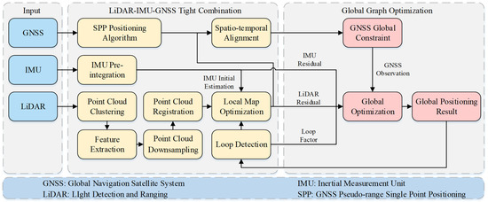
Figure 1.
General framework of the algorithm. LIO’s pose estimation results are used as local optimization factors, and GNSS pseudo-range single point positioning (SPP) results are used as global optimization factors for global constraint.
The front-end of the system is mainly used to preprocess IMU observations and LiDAR original point cloud sequences, and to optimize the generation of local maps by inter-frame matching. The LiDAR raw point cloud sequence is clustered and segmented by a breadth-first-search combined with the Euclidean angle threshold, and then edge and plane feature point clouds are extracted. These two types of feature clouds are downsampled for point cloud alignment, and the local inter-frame matching is optimized using the IMU pre-integration as the initial pose estimate. Finally, the LIO local pose estimates are used to pre-process the GNSS global observations, including the temporal interpolation alignment of GNSS and LIO local observations and coordinate system alignment, so as to achieve the space–time synchronization among sensors.
The back-end mainly uses the residuals of pose estimates of each sensor to optimize the map. The residual factors from local sensors include the IMU pre-integration and LiDAR observation residual, whereas the global residual factors include the GNSS observation residual and loop residual. It should be noted that the global residual factors are added only when their existence is detected, and, when there is no global residual factor, the system only performs local position, such as when the carrier is travelling in a flat and straight tunnel environment. When global corrections are available, the obtained global positioning results are used to update the local pose estimates in the sliding window to obtain the best pose estimates with local accurate registration and global drift-free.
3. Point Cloud Voxelization Downsampling and Alignment
The accuracy of the registration of the environmental point cloud extracted by LiDAR strictly affects the result of the subsequent local pose estimation. Therefore, the processing steps of the front-end point cloud of the system need to be described in detail. This paper mainly involves the improved point cloud downsampling method and registration method.
3.1. Voxelized Downsampling Based on Curvature Segmentation
This paper presents a voxelized downsampling method based on curvature segmentation. Given a set of raw point cloud sequences collected by LiDAR, all points in the raw point cloud sequences are traversed and coarse clustering is performed using a breadth-first algorithm. Furthermore, the geometric angle threshold based on Euclidean distance is used to finely segment the point cloud clusters with similar depth. Let the scanning center of LiDAR be and the two adjacent edge points and in the point cloud cluster with depths and , respectively (). Let the number of point clouds in the point cloud cluster where point is located be . Then, the roughness of point cloud is:
Set the roughness threshold as , then traverse . We classify the points of as the set of edge feature points, classify the points of as the set of plane feature points and perform downsampling operations on them, respectively.
This method is mainly used in the feature extraction step of LiDAR odometry [4]; we extend it to the downsampling step. This means that, for any application where downsampling of point clouds is required, such as artefact inspection, the method can better restore the spatial distribution properties of point clouds by downsampling in clusters.
Next, this paper proposes a point cloud downsampling strategy based on HashMap, instead of the random sample consensus (RANSAC), so that the downsampling result of the point cloud is closer to the approximate center of gravity of voxels. Let the coordinate of a feature point in a set of point cloud sequences in the voxel space be . If the voxel grid size is , the dimension of the voxel grid in the direction is , and the index of in the direction within the voxel grid is . The same applies to the and directions.
After obtaining the 3D index of feature points in the voxel space, if the random sorting strategy of [11] is adopted, the sorting complexity will be , which has a negative impact on the down-sampling time. Therefore, this paper uses the hash function to sort the index of feature points quickly and map them to containers . The hash function is:
To avoid hash conflicts, set the conflict detection conditions as follows:
Once the hash conflict is detected, the index value in the current container is output and the container is emptied, and the new index value is put into the container.
To sum up, the main improvement of this section lies in extending the curvature segmentation step originally used for feature extraction to the downsampling step, and using hash mapping instead of the random sampling method for point cloud sampling. For the LiDAR odometer, using the clustering line and surface features again after the feature extraction step can improve the accuracy of downsampling single-frame or discontinuous point clouds at a weak time cost, thus providing more accurate point cloud distribution results for the pose estimation step between consecutive frames. In addition, using HashMap to downsample can further improve the sampling efficiency, and the time consumption of quadratic curvature segmentation is almost negligible. For other applications that need to downsample point clouds, the point cloud clustering method based on curvature segmentation can restore the spatial distribution of point clouds more accurately, and the benefits of this method are extensive and obvious.
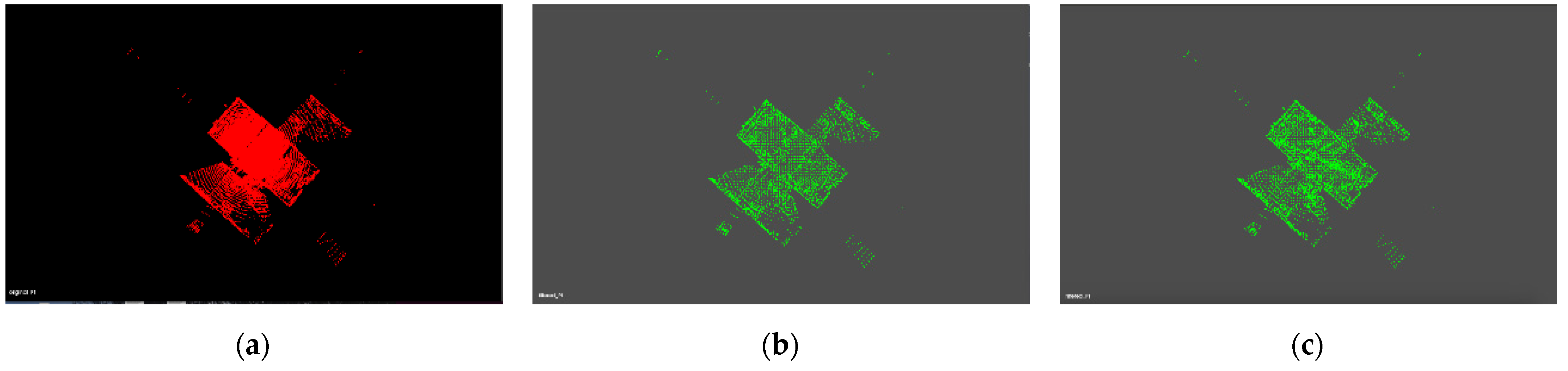
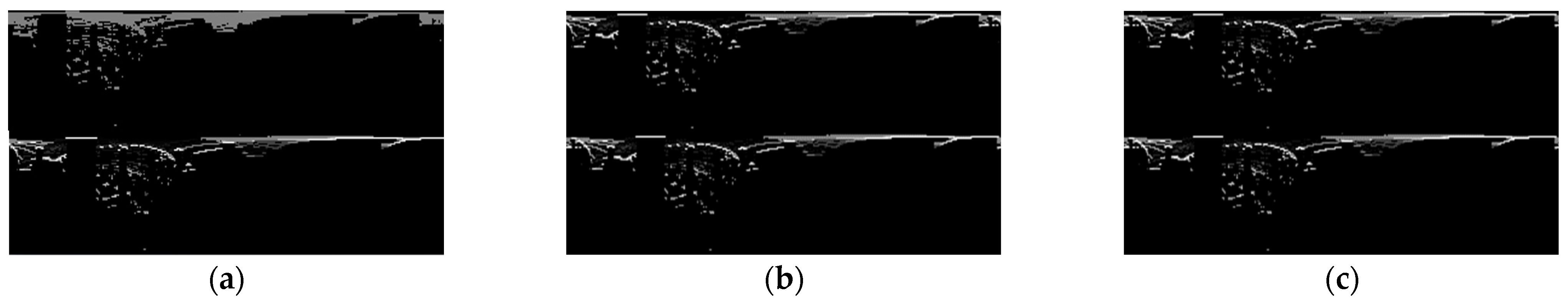
The results and time consumption of the improved point cloud downsampling process are shown in Figure 2 and Table 1. Cloud number , the line feature extraction threshold is 1, the surface feature extraction threshold is 0.1 and r = 0.3. It can be seen from Figure 2c that the present method has a clearer reduction in the spatial distribution of diagonal lines within a rectangular point cloud. Therefore, it can be proved that our method can retain the texture feature information of the source point cloud to a greater extent, and the accuracy and real-time performance of the downsampling results can be improved.
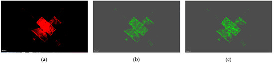
Figure 2.
Comparison of point cloud downsampling results. (a) Source point cloud; (b) downsampling results before improvement; (c) downsampling results after improvement.

Table 1.
Comparison of the number of point clouds and time consumption after downsampling.
3.2. Voxelized Point Cloud Registration
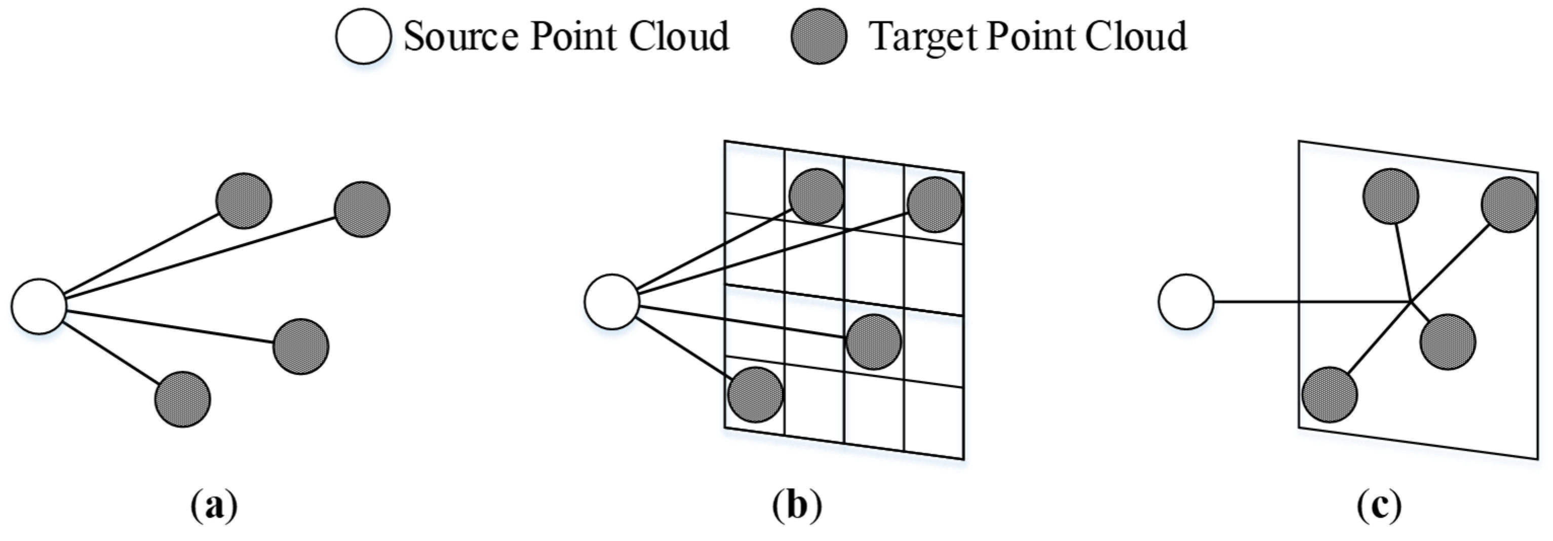
The purpose of point cloud registration is to update the rigid frame transformation of a moving carrier by comparing two consecutive frames of point clouds or similar point clouds detected by a loopback to solve for the carrier’s pose. Traditional LIO usually uses ICP to realize the precise registration of point clouds. The ICP can be briefly described as follows: given a set of source point cloud and target point cloud , the nearest neighbor search of KDTree is used to obtain the inter-frame pose transformation relationship , and the optimal solution is achieved through multiple iterations. However, an unreasonable initial position selection will make ICP fall into the misunderstanding of the local optimal solution, and the calculation resource consumption of the single-point nearest neighbor search is large. In view of the defects of the ICP algorithm, this paper utilizes a method based on the distribution of feature points in voxels, as shown in Figure 3.
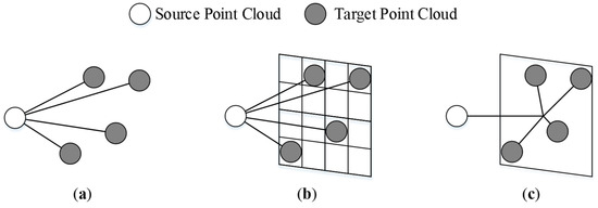
Figure 3.
Comparison of point cloud registration strategies. (a) ICP/GICP; (b) NDT; (c) our algorithm.
As shown in Figure 3. the problem of constructing the nearest neighbor model of a point pair by using a tree diagram is transformed into constructing the nearest neighbor model of a point and a neighborhood point set. Firstly, the two sets of point cloud sequences are approximated as Gaussian distributions, i.e., and , where . and are covariance matrices of two sets of point cloud sequences, respectively. Let the distance between a pair of corresponding points between the target point cloud and the source point cloud be:
Let the neighborhood point set of be , where is the neighborhood judgment threshold. Thus, the distance between the extended point and the neighborhood point set is:
As a result of and , the rigid body transformation error is calculated as:
In this way, the smoothing of all neighboring point clouds in the neighborhood of is achieved. Let and ; because is a high-dimensional Gaussian distribution, its probability density function expansion form is:
The negative logarithmic form of Equation (7) is:
Solving the inter-frame pose transformation matrix T by maximum likelihood method:
Furthermore, after introducing the number of point clouds in the neighborhood , Equation (9) can be written as:
In addition to the smoothing of all neighboring point clouds in the neighborhood of , an iteration termination threshold was established to avoid falling into a blind region of local optima after multiple iterations as follows:
where and are the root mean square error of the previous iterations and the previous iterations, respectively. The iteration is completed when the absolute value of the change in the root mean square error , or the maximum number of iterations, is reached.
4. Graph Optimization Framework
4.1. Local Pose Map Structure
Authors should discuss the results and how they can be interpreted from the perspective of previous studies and of the working hypotheses. The findings and their implications should be discussed in the broadest context possible. Future research directions may also be highlighted.
The local state vectors in the local coordinate system in which the LiDAR and IMU are located are given as follows:
where denotes the state quantity after pre-integration of the th IMU at , including position , rotation , speed and IMU bias , . is the distance from the LiDAR feature point at to the matching edge feature at , and is the distance from the feature point at to the matching planar feature at .
From this, the Gauss–Newton method can be used instead of the fastest gradient descent method used in [27] to minimize all cost functions so as to reduce the number of iterations for rapid convergence to a locally optimal estimate. The local optimization function is constructed as follows:
where is used to solve the carrier pose in the local coordinate system of LiDAR at time . and are IMU measurement residuals and covariance matrices, respectively. The meanings of the terms are described below.
4.1.1. IMU Pre-integration Factor
Let be the IMU pre-integration calculation value between the th and th LiDAR key frames. Details of the derivation of the IMU pre-integration are presented in Appendix A. is the time interval between the two LiDAR key frames, and the spatial transformation matrix from the IMU coordinate system to the LiDAR coordinate system in th frame is represented by . The IMU residual can be obtained as follows:
where the symbol represents extracting the real part of the quaternion used to calculate the rotation state error, and represents the quaternion multiplication.
After the pose estimation of the previous key frame is completed, the IMU acceleration bias and gyroscope bigotry will be updated, the update amounts are set as and and the pre-integration calculation value at this time is updated as follows:
4.1.2. LiDAR Factor
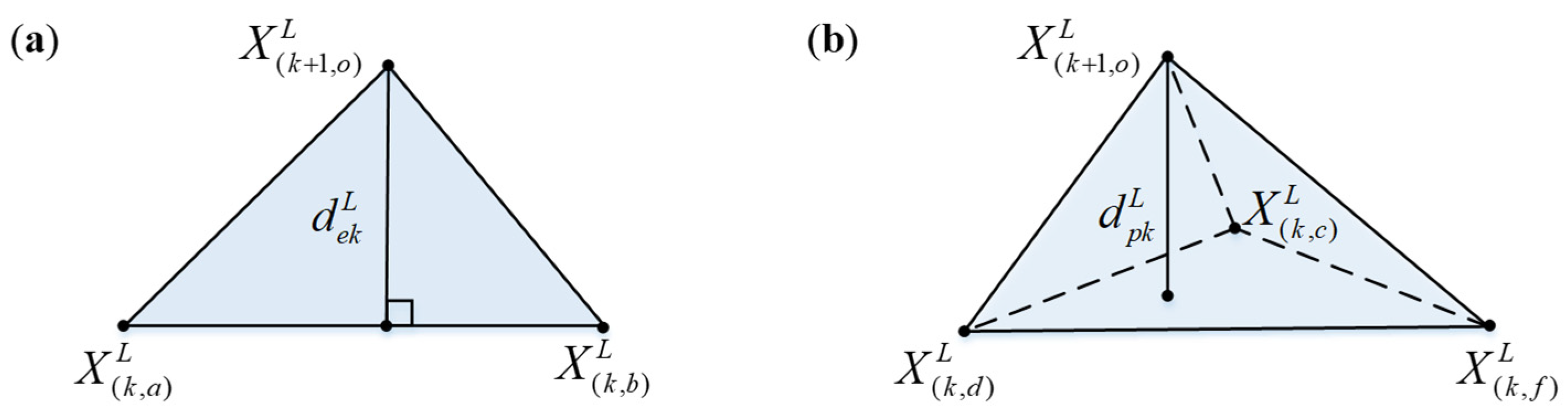
The feature point cloud extracted by LiDAR can be divided into two types: line features and surface features. The LiDAR residuals of the two types need to be constructed separately and then summed to obtain the total LiDAR residuals. Details of the specific derivation of LiDAR residuals are presented in Appendix B. Figure 4 shows the schematic diagram of LiDAR residual construction.

Figure 4.
Schematic diagram of LiDAR residual construction. (a) Line characteristic residual construction; (b) surface characteristic residual construction.
As shown in Figure 4, let a feature point obtained in the th scan have the coordinates of in the LiDAR coordinate system, and the coordinates of two end points of the line features matched with it in the th scan are and . The residual error of the line features can be expressed by the point-to-line distance:
Similarly, if the surface features that match it in the th scan are represented as , and , then the surface feature residual can be represented by the point-to-surface distance:
4.2. Spatial Unification of Multi-Sensor Poses
Constructing the time—space correlation of each sensor is a fundamental task in multi-sensor fusion optimization. For this system, it is necessary to spatially unify the positional estimation results of LiDAR and IMU in the local map with the GNSS measurements in the global map. Therefore, the spatial unification strategy of the multi-sensor pose involved in this paper is shown in Figure 5.
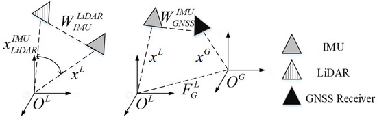
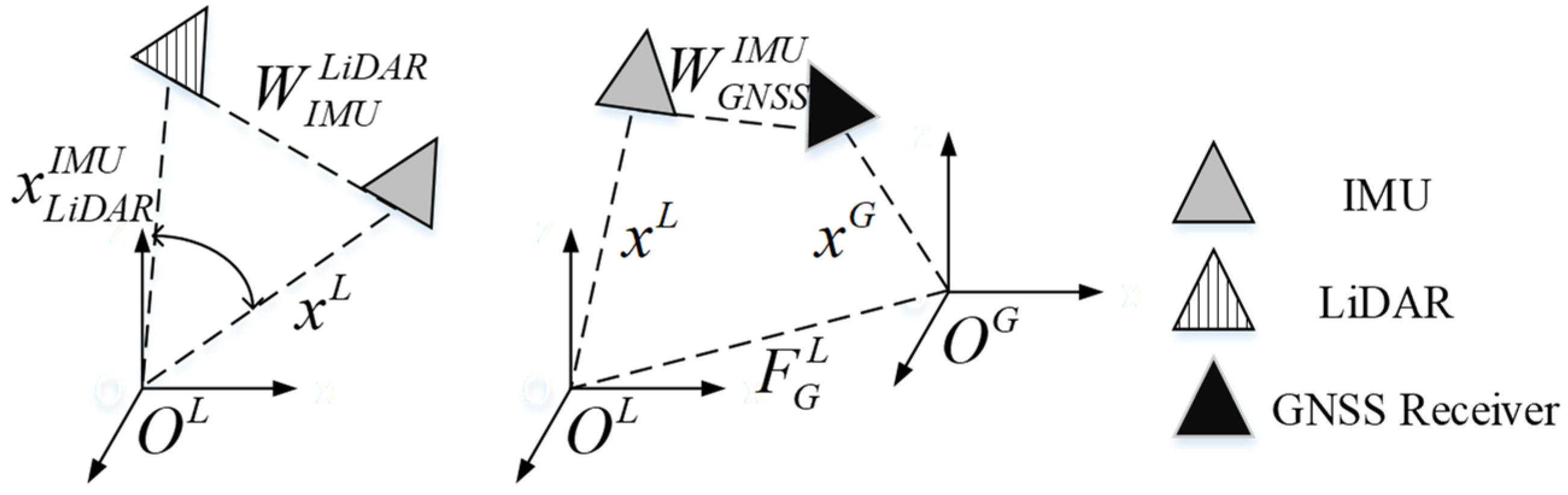
Figure 5.
Schematic diagram of the spatial unification of multi-sensor poses. The spatial association of the poses of LiDAR and IMU in the local coordinate system is on the left, and the spatial association of the poses of IMU and GNSS receivers in the global coordinate system is on the right.
As shown in Figure 5, is the external parameter conversion matrix from IMU to GNSS and is the external parameter conversion matrix from LiDAR to IMU. Since the hardware is fixed to the mobile carrier, both are calibrated to a constant value. The left figure shows the positional conversion between LiDAR and IMU in the local coordinate system, whereas the right figure shows the multi-sensor positional spatial unification from the local to the global coordinate system. Here, it is necessary to introduce the spatial transformation parameters (including translation and rotation ) to correlate the two positional spaces. The spatial unification of the multi-sensor pose at the moment of can be expressed as:
where the initial value of is set as the unit matrix. Every time the GNSS factor is added to solve the global optimum, the value of at the next moment will be updated, thus correcting the cumulative offset between the local and global coordinate systems.
4.3. Global Pose Map Structure
Global pose map construction can be regarded as a nonlinear optimization problem; that is, the nonlinear optimization of the state vector in the sliding window. Different from the factor graph method adopted in [27], this paper adopts the graph optimization method to directly construct the residual block in the original pose graph structure for nonlinear optimization, and only optimizes the key frames in the sliding window. However, the factor graph based on GTSAM [29] needs to construct the optimization problem into a new graph corresponding to the original pose graph, with the optimization variables as the vertices and error terms as the edges. The complicated constraint relationship among the vertices is more favorable toward the optimization accuracy. However, once a new key frame is detected, all of its associated constraint nodes will be updated, which is complicated and takes too long in the engineering field. Therefore, in order to meet the requirements of the lightweight and real-time performance of the vehicle platform, we choose not to build a new constraint-related Bayesian network, but to construct the residual error and nonlinear optimization in the original pose map structure. The global pose optimization framework proposed in this paper is shown in Figure 6.
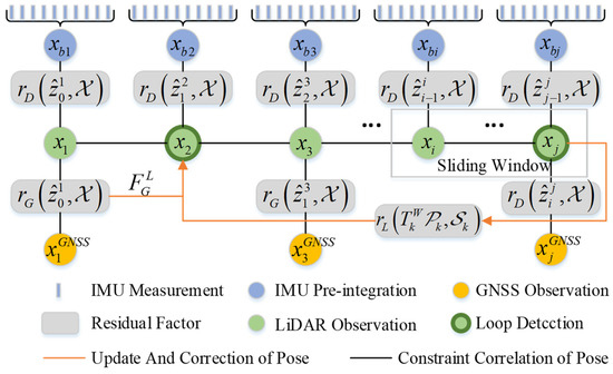
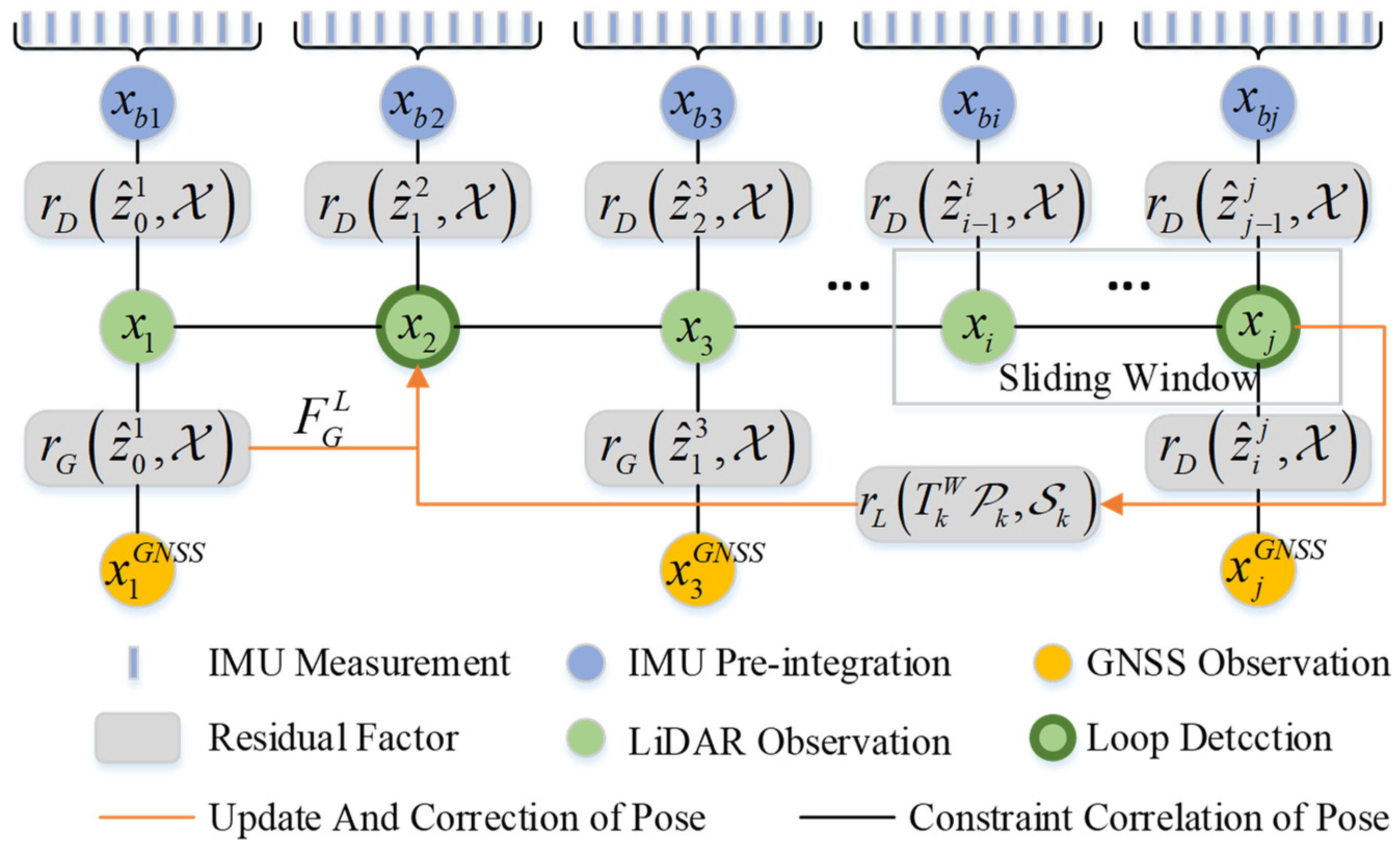
Figure 6.
LiDAR-IMU-GNSS fusion framework based on graph optimization.
The global optimization function is constructed as follows:
where is the GNSS confidence level expressed by the covariance of the error in the GNSS observations obtained by the pseudo-range single point positioning (SPP) algorithm solution. is the pose transformation matrix between the current global point cloud and the local point cloud derived from the inter-frame local matching. The specific meaning of each sensor cost function in the formula are as follows.
4.3.1. LIO Factor
According to Section 4.1, the position and rotation of the carrier in the local coordinate system at the moment can be obtained. Therefore, the LIO local residual factor can be constructed as follows:
where the symbol represents the quaternion subtraction.
4.3.2. GNSS Factor
Set the time interval between two frames of GNSS observations as and realize the time alignment with LIO pose estimation by interpolation. Cubic spline interpolation is used for position interpolation and spherical linear interpolation is used for quaternion interpolation. Now, given the GNSS measurement in the ENU coordinate system and the LIO positional observations in the global coordinate system, the GNSS residual factor is expressed as follows:
When the carrier moves to the GNSS signal confidence region, in order to fully and reliably utilize the GNSS observations, the GNSS factor is added with the GNSS confidence as the weight. The GNSS confidence is determined by the number of visible and effective GNSS satellites. After GNSS participates in the global pose estimation, it will update the pose conversion parameter between the local coordinate system and the global coordinate system. This ensures that, even if the mobile carrier enters a GNSS-rejected environment (e.g., indoor car parks and tunnels), our algorithm can provide a more accurate initial observation after GNSS correction.
4.3.3. Loop Factor
Considering the possible overlap of the moving vehicle driving areas, it is necessary to add a loop detection link to establish possible loop constraints between non-adjacent frames. According to Equation (5), the loop factors can be constructed as follows:
Using the optimized point cloud registration method in Section 3.2, we optimize and correct the historical trajectory through the registration between the point cloud of the prior local map and the current global point cloud. This method ensures that the positional estimates converge to the global optimum result.
5. Experimental Setup and Results
5.1. Point Cloud Registration Results
To verify the superiority of the point cloud registration algorithm used in this paper, we compared the registration results of the ICP algorithm used in traditional LiDAR odometry with our algorithm. The comparison results are shown in Figure 7, Figure 8 and Figure 9.
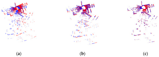
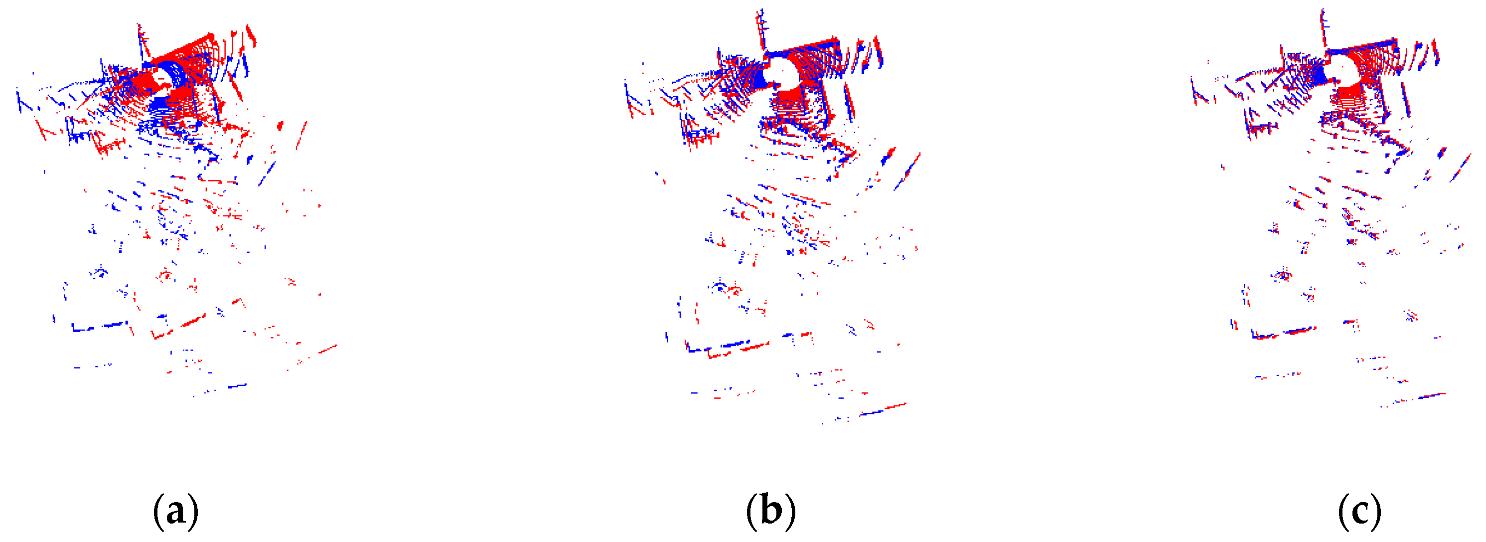
Figure 7.
Point cloud registration results. (a) Original source and target point clouds. (b) Alignment results using ICP algorithm. (c) Alignment results using our algorithm.
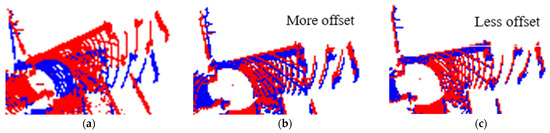
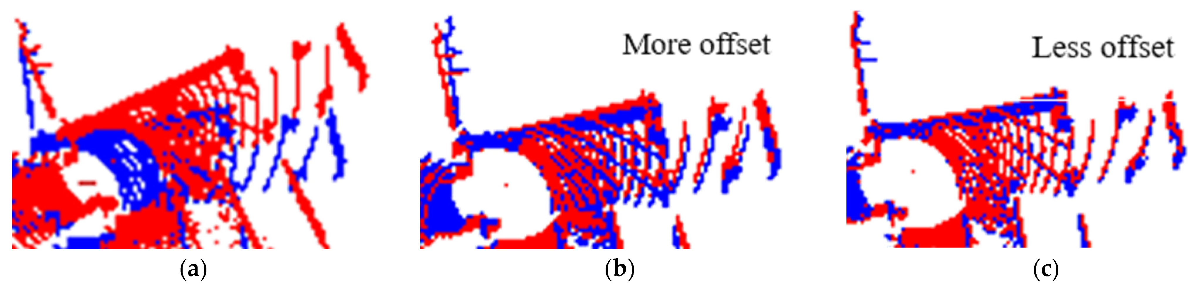
Figure 8.
Detail diagram of point registration results of the point cloud registration results. (a) Original source and target point clouds. (b) Alignment results using ICP algorithm. (c) Alignment results using our algorithm.
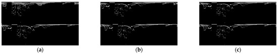
Figure 9.
A circular expansion of the point cloud alignment results. (a) Original source and target point clouds. (b) Alignment results using ICP algorithm. (c) Alignment results using our algorithm.
Compared with the typical indoor environment, for mobile carriers in complex urban environments, the angles and translations between the source and target point clouds during the continuous frame and the loopback detection may be larger. As shown in Figure 7, when the initial position is unreasonable, the registration results of the ICP algorithm cannot fully approach the global optimal solution, which is detrimental to both the local pose estimation and loopback correction of the mobile carrier. However, the registration accuracy of our algorithm is not affected by the large positional transformation of the vehicle platform. Compared with the traditional ICP algorithm, the registration result of our algorithm suited the needs of the vehicle platform better.
Furthermore, in order to avoid the contingency of the registered objects, we made a comparative experiment on the source point clouds with different rotation angles and translation distances, and quantitatively compared the registration accuracy and time consumption of each algorithm. The test results are shown in Table 2 and Table 3.
Table 2.
Registration results of different algorithms for point clouds with different angles.
Table 3.
Registration results of different algorithms for point clouds with different translation distances.
From the vertical comparison between Table 2 and Table 3, it can be seen that the point cloud registration algorithm is more sensitive to rotation, which means that, if the vehicle rotates at a large angle in the city, the point cloud registration between consecutive frames is perhaps less reliable. It may even lead to a failure of the pose estimation, as has been demonstrated in [5]. However, as the rotation angle increases, it can be seen from Table 2 that the registration accuracy of our algorithm decreases the least, and, at the extreme 90° rotation angle, the accuracy is still more than four times better than the other algorithms, with a root mean square error of approximately 2.67116 m. On the other hand, for large translations (5 m) between the source and target point clouds, our algorithm also shows an excellent registration accuracy, with a root mean square error of approximately 0.03047 m. It is worth noting that, in the aspect of single-point cloud registration, the registration time of our algorithm is increased by approximately one order of magnitude compared with others. To sum up, it is sufficient to verify the superiority of the proposed registration algorithm in terms of compressing time and improving the registration accuracy.
5.2. Positioning Accuracy
In this paper, the absolute trajectory error (ATE) was selected as the evaluation index of SLAM system positioning accuracy so as to directly reflect the difference between the global position estimation of the moving carrier and the ground truth. The absolute trajectory error is calculated as follows.
where is the absolute trajectory error of the SLAM system in the th frame, and are the ground truth and the estimated pose, respectively, and is the transformation matrix between the ground truth and the estimated pose. In this paper, the mean error (ATE_ME) and root mean square error (ATE_RMSE) of the absolute trajectory error were selected as evaluation criterion.
5.2.1. Public Dataset
To verify the positioning accuracy of the fusion algorithm in different outdoor environments, the KITTI_RAW dataset [30], which includes a variety of outdoor scenes, was used to evaluate the localization accuracy of the fusion algorithm and to compare it with other similar advanced algorithms. The experimental data acquisition platform is as follows: LiDAR point cloud data are acquired by Velodyne HDL~64 line LiDAR, with horizontal field angle of view of , vertical field angle range of , horizontal resolution range of , vertical angle resolution of and scanning frequency of 10 Hz, which can meet the requirements of in-vehicle point cloud data acquisition. The GPS/IMU integrated system adopts OXTS RT3003, with a GPS output frequency of 1 Hz/s and an IMU output frequency of 100 Hz. The ground truth is provided by a high-precision integrated navigation system.
Four different outdoor scenarios were used to validate the performance of the fusion algorithm, including urban environments, open area, highway and forest road. The voxel grid size of the fusion algorithm was set to 0.3 × 0.2 × 0.3, the maximum iteration threshold was set to 30 and the iteration termination tolerance threshold was set to 1 × 10⁻⁸, so as to meet the real-time requirements and ensure the stable number of feature point clouds participating in the matching in sparse areas of outdoor environments. The comparison of the experimental results is shown in Figure 10 and Figure 11 and Table 4.
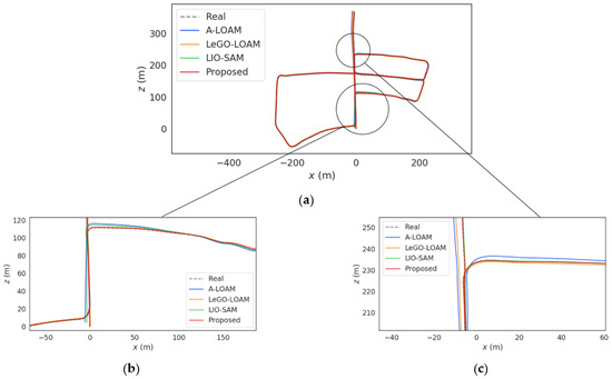
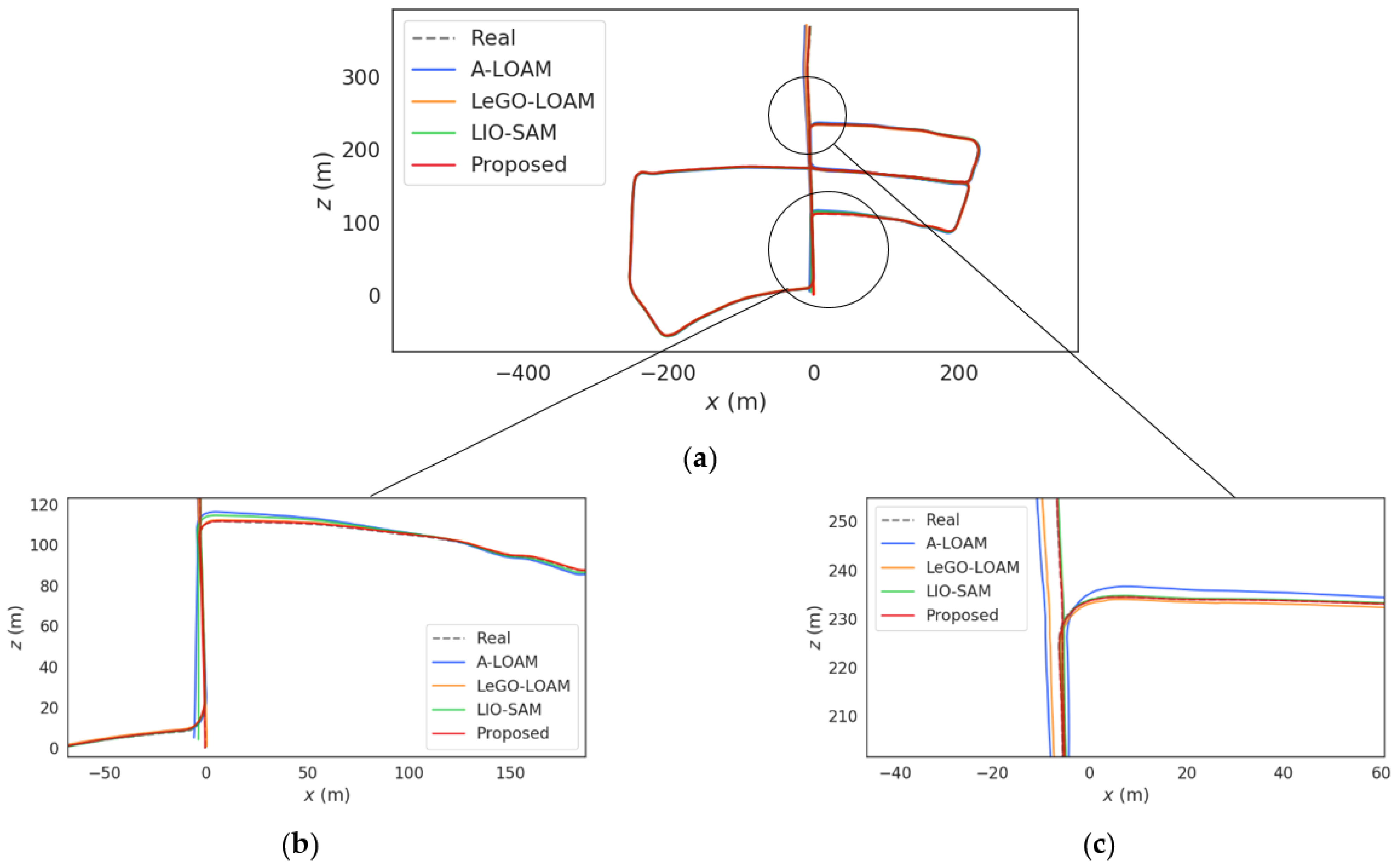
Figure 10.
Comparison of the estimated trajectories. (a) Global positioning trajectory. (b) Local details of the trajectory. (c) Local details of the trajectory.
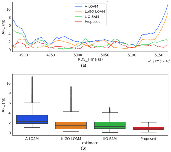
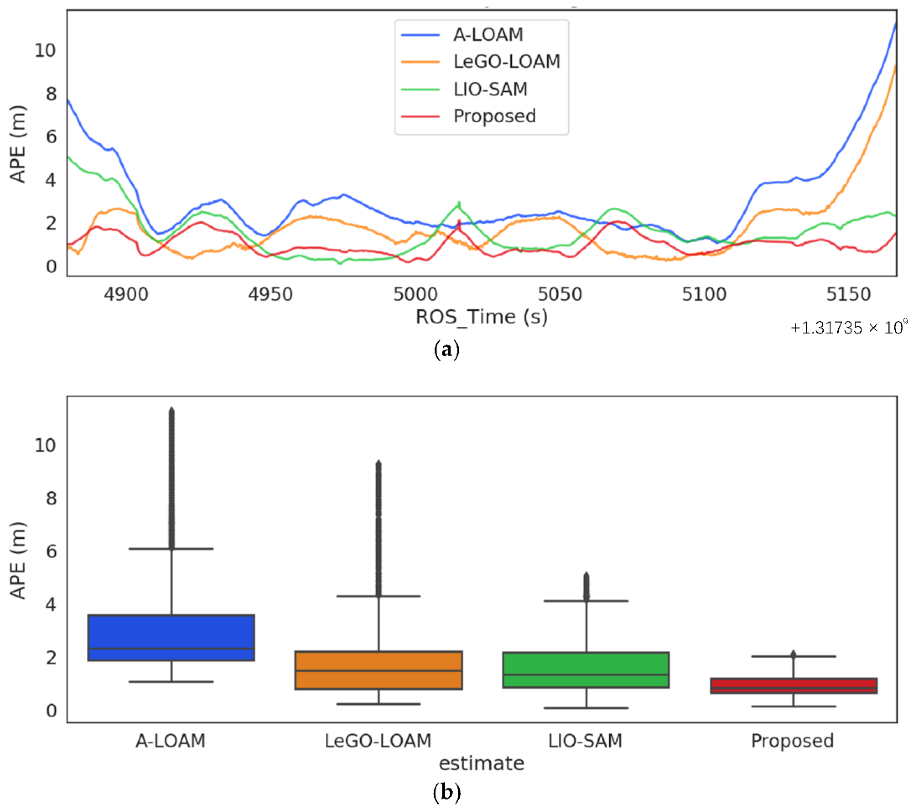
Figure 11.
Comparison of the positioning error of each algorithm. (a) APE fitting curve. (b) The box diagram of APE.
Table 4.
Comparison of ATE_RMSE(m) of each algorithm in KITTI_RAW dataset.
Figure 10 shows the comparison of the positioning results of each algorithm in the 09_30_0018 dataset representing the urban environment. As shown in Figure 11b, both LiDAR odometry (LO), represented by A-LOAM, and LIO, represented by LeGO-LOAM, show significant degradation in the position estimation results in the first 50 s and the last 50 s. The reason is that LO and LIO systems only rely mainly on LiDAR to extract spatial geometric feature information. Once LiDAR feature constraints are sparse or fail, the carrier state estimation degradation will occur in this feature direction, and additional constraints need to be added. The first 50 s and last 50 s are both flat, open roads with sparse point cloud features, which are susceptible to the degradation of the LiDAR positional optimization results. However, the number of GNSS visible satellites in the flat and open road is enough, and using GNSS observations as global constraints can greatly improve the positioning accuracy and robustness in sparse areas of point clouds. As can be seen from Figure 11b, the ATE_RMSE of both the LIO-SAM with GNSS global constraints and the present algorithm is stable between (0 m, 2 m), and the positioning accuracy remains stable in the sparse region of the point cloud features in the latter 50 s without large data drift. In addition, from the box diagram shown in Figure 9c, it can be seen that the positional outliers estimated by LIO-SAM are reduced by approximately 80% compared with the LIO system. Furthermore, the positional estimation errors of our algorithm are concentrated between (0.68 m, 1.23 m) with very few outliers, which fully demonstrates the superiority of the proposed algorithm in its positioning accuracy in urban environments.
5.2.2. Urban Dataset
To further investigate the extent to which improvements in both the front-end and back-end components of the fusion algorithm improve its positioning accuracy, we conducted ablation experiments in a complex environment of GNSS signals. We constructed a system without GNSS global correction (-), a system without smoothed voxelized point cloud registration and loopback correction (#) and a complete system (Proposed), respectively. The experimental environment is the complex reflection area of GNSS in the urban environment. The experimental platform includes: the ground truth, which is provided by NovAtel SPAN-CPT positioning results; the LiDAR point cloud, which is acquired by HDL 32E Velodyne LiDAR, where the horizontal field of view angle is , the vertical field of view angle range is and the scanning frequency is 10 Hz, which is suitable for in-vehicle point cloud data acquisition; IMU, which is Xsens Mti 10, and the update frequency of the pose is 100 Hz; the GNSS receiver, which is u-blox M8T, and the update frequency is 1 Hz.
Different from the KITTI_RAW dataset, the GNSS confidence parameter in this experiment is not fixed. After solving the raw observation data collected by u-blox with the SPP algorithm, we obtained the GNSS confidence covariance as the GNSS factor weight parameter. This is more in line with the real urban environment, where GNSS reflected and refracted signals interfere with the direct signal superimposed, thus causing the pseudo-range and carrier phase observations to deviate from the true value of the direct signal. The experimental results are shown in Figure 12 and Figure 13 and Table 5.

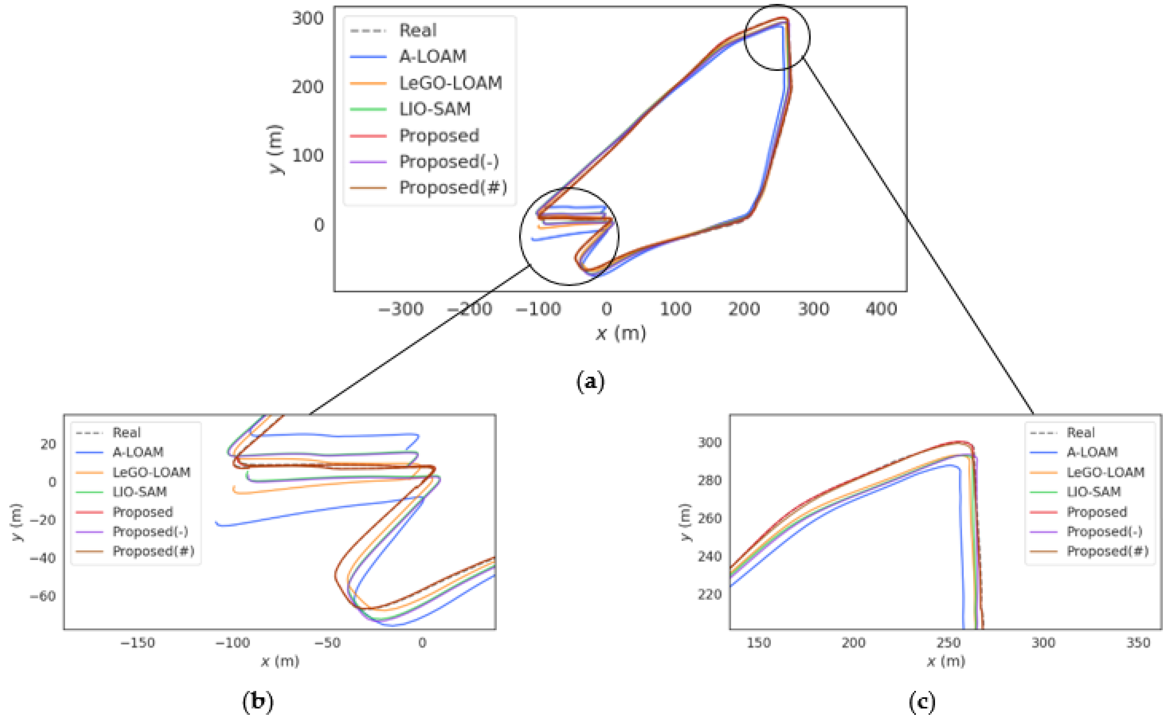
Figure 12.
Comparison of the estimated trajectories. (a) Global positioning trajectory. (b) Local details of the trajectory. (c) Local details of the trajectory.
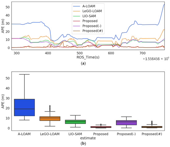
Figure 13.
Comparison of the positioning error of each algorithm. (a) APE fitting curve. (b) The box diagram of APE.
Table 5.
Motion estimation errors of each algorithm on outdoor dataset.
As can be seen from Figure 13a, firstly, due to the accurate registration of the front-end point cloud, the absolute trajectory error of Proposed(-) decreases slightly compared to the pre-improved system. In the initial parking section of the dataset, the traditional ICP algorithm suffers from the problem of over-iterations, and the result is not the global optimal solution. However, the data smoothing processing and the setting of the iteration termination threshold of our algorithm can solve this problem well, providing a better initial value for the positional matching. The absolute trajectory error within the first 25 s drops by approximately 8m compared to LIO-SAM. Secondly, compared to LIO-SAM, which uses GNSS observations directly as global constraints without filtering, we introduced GNSS confidence into the optimization equation. It allows our algorithm to remain unaffected by poor-quality GNSS observations and to maintain a better positioning accuracy in the latter 50 s in areas with dense tall buildings and poor-quality point cloud distribution. In contrast, due to the poor quality of GNSS observations involved in optimization (LIO-SAM) and the low accuracy of LiDAR loop detection as a global constraint (A-LOAM and LeGO-LOAM), all other similar algorithms have a cumulative increase in the absolute trajectory error with steeper slopes. This is extremely detrimental for vehicle-mounted platforms driving in realistic large outdoor environments. From the experimental results, it can be seen that the global optimization link in our complete algorithm can well suppress the local cumulative drift and make the pose estimation result move more towards the global optimal solution.
In summary, driven by a combination of respective front-end and back-end improvements, our complete algorithm achieves a higher positioning accuracy than other comparable algorithms within real urban environments. Furthermore, as a result of the inherent advantage of local sensors not being subject to signal refraction environmental interference, it compensates for positioning outliers arising from multipath effects in traditional GNSS positioning in urban environments. It fully ensures the integrity and reliability of the fusion system’s positioning.
5.3. Time-Consuming Performance
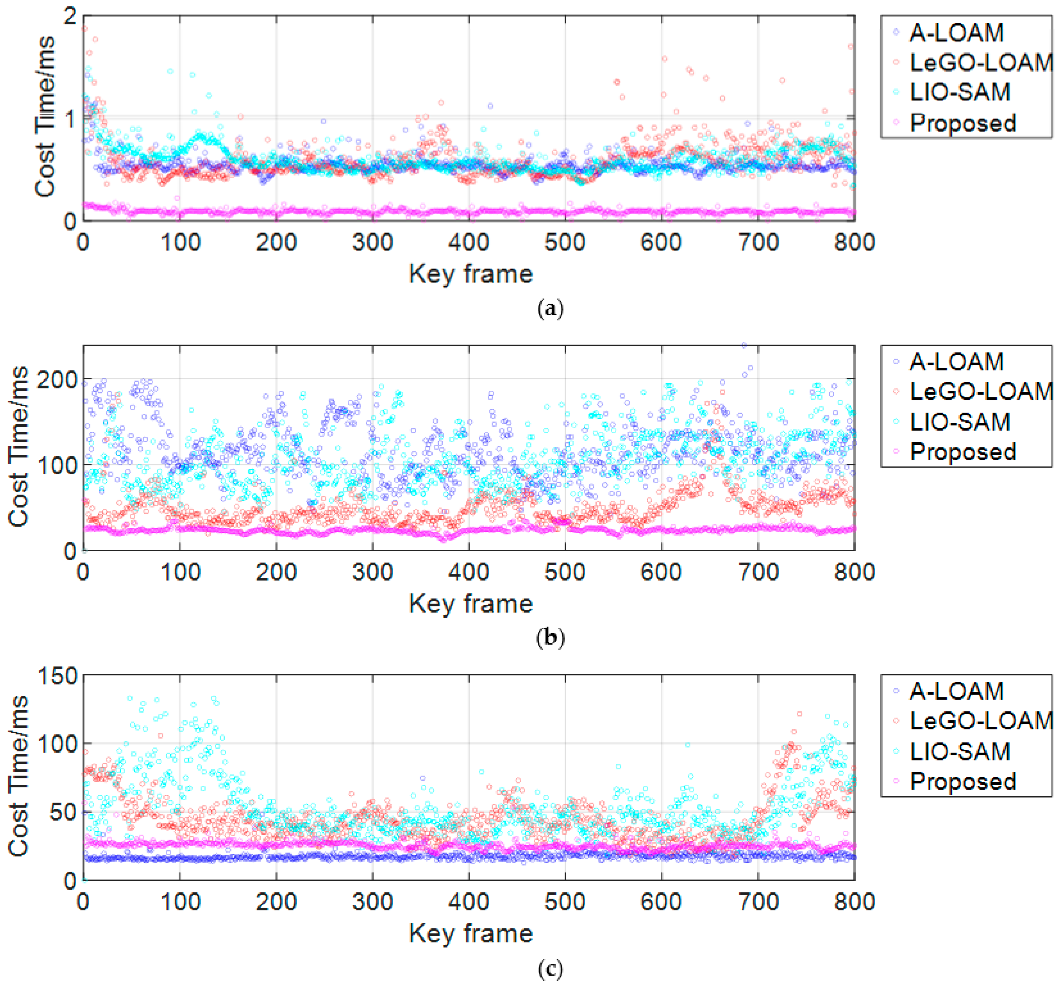
In this paper, the KITTI 09_30_0033 sequence is randomly selected to verify the real-time performance of our algorithm and the similar algorithms. In this paper, the above-mentioned three similar advanced algorithms are selected as control algorithms to compare with our algorithm, so as to verify the superior real-time performance of this algorithm in three stages: downsampling, point cloud registration and optimization. The experimental results are shown in Figure 14.
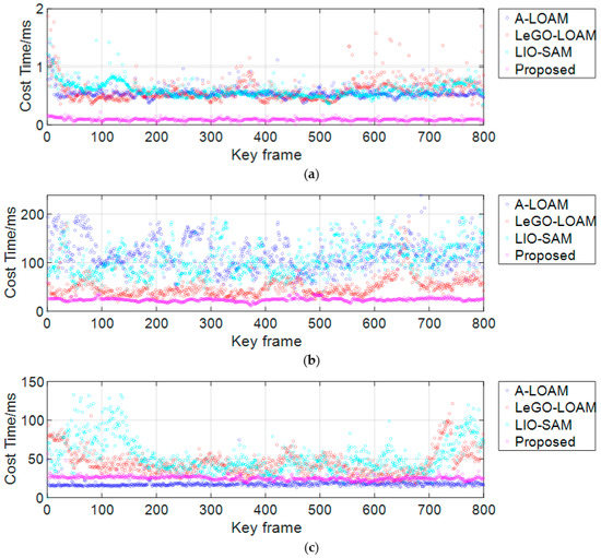
Figure 14.
Time-consuming comparison of three processes. (a) Point cloud downsampling process. (b) Point cloud registration process. (c) Position global optimization process.
The time consumption of the point cloud downsampling is shown in Figure 14a. The downsampling process of the three other algorithms uses RANSAC as the core algorithm, but its iterative approximation speed is slow, at approximately (0.5 ms, 1 ms), and the filtering and fitting quality of the depth information is not good. In contrast, our proposed algorithm uses HashMap instead of random sampling, which improves the speed of filtering out similar points in voxels to a certain extent and reduces the time consumption by two to five times compared with the traditional downsampling method. Although the time-consuming ratio of this process is relatively small in typical indoor environments or short-term positioning processes, for vehicles driving in large outdoor environments with complex point cloud environments for long periods of time, the accumulation of tiny instances of time consumption will lead to a cumulative increase in positioning time consumption. Therefore, the time-consuming compression in point cloud downsampling in this paper is beneficial for ensuring real-time vehicle positioning.
The time consumption of the point cloud registration is shown in Figure 14b, which shows that the time taken for the LIO-SAM and A-LOAM point cloud registration step is in the range of (50 ms, 200 ms). By extracting and separating the ground point clouds, LeGO-LOAM can inhibit the time-consuming increase caused by outlier registration due to the interference between non-identical cluster point clouds to a certain extent. The point cloud registration step takes approximately (50 ms, 100 ms). There are two possible factors for the obvious fluctuation of the above algorithm. The first is the fluctuation in the registration time due to the changing distribution of the ambient point cloud. The second is that, according to the experiments in Section 5.1, the rotation angle and displacement between the source and the target point cloud also have a certain influence on time consumption, which is obvious in the urban driving environment, where the speed and driving direction change irregularly. However, the time consumption of our algorithm is stable between (20 ms, 30 ms). The smoothing of the single-to-many distribution of the point cloud sequence greatly reduces the effect of the sparsity of the point cloud distribution on the alignment time, ensuring that the point cloud alignment step is both time-efficient and stable.
The time consumption for the positional optimization step is shown in Figure 14c. The time taken to match the local map to the global map for LIO-SAM and LeGO-LOAM is around (30 ms, 130 ms). Due to the addition of GNSS sensors and the interference of some GNSS observations with low confidence, the total time consumption of LIO-SAM is even higher than that of LeGO-LOAM. However, A-LOAM takes (20 ms, 25 ms). The main reason is that the observation of only one sensor in LiDAR needs to be optimized, and the residual block is directly constructed in the original pose map structure, which reduces the computational burden of the multidimensional factor map. In this algorithm, the optimization method of A-LOAM is used for reference. It can be seen that, although the GNSS sensor is added, the time consumption is still stable at approximately 30 ms. The reason is that the global constraint of GNSS provides a more accurate transformation matrix from the local map to the global map for the fusion system, which makes it easier for the objective function of map matching to converge to the optimal solution. Secondly, we use the Gauss–Newton method instead of the steepest gradient descent method used in [27] to minimize all of the cost functions, so as to reduce the number of iterations to converge quickly to the locally optimal estimate, which is one of the main reasons for the decrease in time consumption. The average total time of each algorithm in a single frame is shown in Table 6.
Table 6.
Comparison of average total time consumption of each algorithm in single frame.
In summary, thanks to the double improvement of this algorithm in the front-end and back-end of our system, the time consumption of all three steps involved is compressed. Although the optimization vector of the GNSS sensor is newly added, it has a better real-time performance than other similar algorithms.
5.4. Mapping Results in the Real Urban Environment
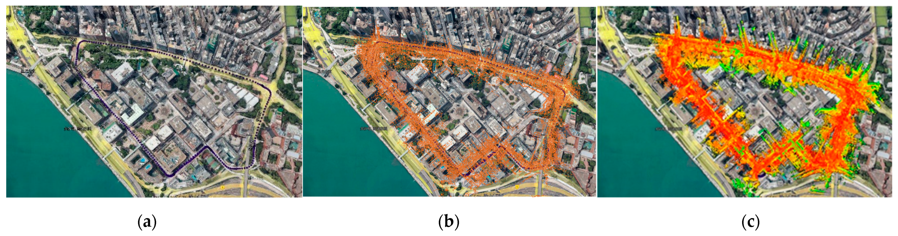
As shown in Figure 15, this section shows the comparison of mapping results between our algorithm and similar advanced algorithms. Figure 15a shows the ground truth in the real outdoor environment, which is obtained by NovAtel SPAN-CPT. The vehicle travels for one week from the starting point in the lower right corner and then returns, and the trajectory is almost closed. Figure 15b shows the mapping result of LIO-SAM, and it is clear that the section near the end of the journey deviates significantly from the actual path travelled. The reason can be attributed to the fast displacement of the carrier, which leads to an increased difference in the point cloud clusters captured between the front and back frames, including rotation and displacement, resulting in the point cloud registration in the loopback detection of LIO-SAM being prone to failure and the loopback constraint results not being ideal. In addition, the GNSS constraint strategy adopted by LIO-SAM has a poor global correction effect on local sensors. However, compared with LIO-SAM, our algorithm has an obvious loop detection accuracy and GNSS global constraint effectiveness.
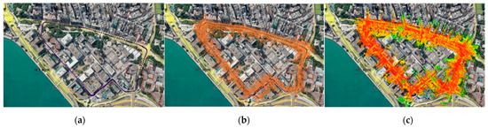
Figure 15.
Comparison of mapping effects of various algorithms. (a) The ground truth. (b) The mapping results of LIO-SAM. (c) The mapping results of the proposed algorithm.
As shown in Figure 15c, the mapping trajectory of the algorithm proposed in this paper is basically fitted with the true value of the driving trajectory, and, in the loop road section in the lower right corner, the trajectories passing through the same landmark twice are basically coincident. The reasons are as follows: firstly, smoothing the point cloud clusters can improve the fault tolerance of the point cloud registration between the front and back frames; secondly, the weighted GNSS global constraint can eliminate the GNSS measurements with large observation gross errors, thus achieving superior mapping results.
6. Discussion
SLAM-based multi-sensor fusion positioning technology expands the application field of traditional GNSS-based mapping techniques and makes continuous and reliable positioning in complex urban environments with good/intermittent/rejection GNSS a reality. The superior sensing capability of LIO for natural sources has been demonstrated in the literature [5,6] and others. However, the accuracy limitation of point cloud registration and the local pose drift of LIO limit the application of LIO in large outdoor environments to some extent. This paper focuses on the above two technical bottlenecks faced by the existing LiDAR SLAM and proposes simplified but effective improvement solutions.
First of all, the primary technical bottleneck is how to improve the accuracy of point cloud registration. Koideet al. [20] demonstrated that smoothing the point cloud cluster can improve the fault tolerance of point cloud registration and improve the accuracy of the point cloud from 1.20m to 0.89m. However, from our practical tests, it has been shown that, in long and large turning or translating sections in real environments, if the number of iterations is not limited, it may still fall into the local optimum problem. Therefore, on the basis of constructing a registration equation based on smooth voxelization filtering, we further use the judgment condition of iteration termination for the secondary constraint, so as to reduce the over-fitting problem of local point clouds in a typical environment. According to the registration experiment in Section 5.1 and the positional estimation accuracy experiment in Section 5.2, it can be seen that our registration method has a higher accuracy than the conventional methods. According to Figure 11, it can be seen that accurate point cloud alignment leads to an accurate initial value estimation of the positional attitude, which has a considerable positive effect on the positional estimation of the vehicle platform with a complex moving state.
Secondly, there is the challenge of how to effectively use GNSS measurements and loopback detection mechanisms to converge the local positioning results of LIO to a globally optimal solution. Firstly, the main step of loop detection dependency is point cloud registration. The previous paragraph has specifically analyzed the superiority of our method. Thanks to the positive point cloud registration results, we can reason that our global constraint using loopback detection is superior, as demonstrated in Section 5.2.2. Next, some related research has been carried out on the research of GNSS and LIO fusion positioning. Optimization-based methods have been applied in [31,32] and so on. However, taking [27] for example, in the traditional graph optimization model, the covariance effect of measurements is only used to determine whether to add factors or not, which is crude for the screening of the measurements, especially for GNSS, a measurement signal that is greatly influenced by the environmental catadioptric surface, where its observation information has not been fully applied. Therefore, in this paper, on the basis of the rough screening of GNSS observations, the covariance of the quantitative measurements is added as a weight to the graph optimization model. It achieves a more adequate and accurate global constraint on the LIO local poses using GNSS observations. From the ablation experiment results in Section 4.3.2, it is evident that the method of the weighted GNSS residual added in this paper achieves a satisfactory positioning accuracy. According to the above results, we can draw a reasonable inference: even when entering an indoor parking lot or tunnel, the accumulated error of LIO in this algorithm will start to accumulate from a lower initial value of drift. In contrast, for the LIO algorithms without GNSS constraints, they already have a large deviation between the local map and the global map before entering the denial environment. Therefore, the cumulative error range of this algorithm is acceptable. Once the GNSS signal is restored, the local error will be corrected within the time alignment interval of 0.1s as set in Section 4.3.2. This provides an accurate and continuous positional estimation for the in-vehicle platform during travel in complex urban environments.
7. Conclusions
In this paper, a LiDAR-IMU-GNSS fusion positioning algorithm with accurate local alignment and weak global drift is proposed for the high-precision continuous positioning of mobile carriers in complex urban environments.
Firstly, a voxelized point cloud downsampling method based on curvature segmentation is proposed. Rough classification is carried out by a curvature threshold, and the voxelized point cloud downsampling is performed using HashMap instead of RANSAC, so that the spatial feature distribution attributes of the source point cloud, including texture feature information, such as surfaces and curves, are retained to a greater extent.
Secondly, a point cloud registration model based on the nearest neighbors of the point and neighborhood point sets is constructed. Furthermore, an iterative termination threshold is set to reduce the probability of the local optimal solution. This greatly improves the real-time performance of the point cloud registration and can also play a large role in aligning the point cloud between the front and back frames of a fast-moving carrier with large displacement.
Finally, we propose a LIO-GNSS fusion positioning model based on graph optimization that uses GNSS observations weighted by confidence to globally correct local drift. In addition, the loop detection mechanism using the above-mentioned point cloud registration algorithm is also added into the fusion system, resulting in further global constraints of the driving areas with prior maps. Experimental results show that our algorithm can realize a more continuous and accurate pose estimation and map reconstruction in complex urban environments than similar state-of-the-art algorithms.
In the future work, there are still several issues in our work that deserve further exploration. Firstly, we plan to build a deeper constraint relationship between LIO and GNSS and make use of the rich planar features perceived by LiDAR in the urban environments to compensate for GNSS occlusion or the presence of multipath areas in the direction of the constraint. It will reduce the probability of the unreliability of SPP positioning results in the urban environments. Secondly, considering the environments with multi-sensor failures, such as tunnels with a high environmental texture similarity, where both GNSS rejection and point cloud degradation failures exist. We consider a more accurate degradation direction detection using the degeneracy factor (DF) algorithm proposed in [5], and make a non-linear optimization correction for the positional attitude in that direction. Finally, the perception ability of 3D environmental features by using only LiDAR, IMU and GNSS sensors is still relatively limited. We plan to use the observation residuals from other sensors to add multi-dimensional feature constraints to the fusion positioning algorithm, such as cameras, wheel odometers and so on, so as to make full use of environmental features and realize accurate and real-time navigation and positioning targets with high environmental universality.
Author Contributions
Conceptualization, X.L.; methodology, X.H.; software, X.H.; validation, S.P.; formal analysis, X.H.; investigation, X.L.; resources, W.G.; data curation, X.H.; writing—original draft preparation, X.L.; writing—review and editing, X.H.; visualization, X.H.; supervision, S.P. and W.G.; project administration, W.G.; funding acquisition, S.P. All authors have read and agreed to the published version of the manuscript.
Funding
This research study was funded by the National Key Research and Development Program of China (2021YFB3900804) and the Research Fund of the Ministry of Education of China and China Mobile (MCM20200J01).
Data Availability Statement
Not applicable.
Conflicts of Interest
The authors declare no conflict of interest.
Appendix A
Mathematical Derivation of the Equations (14) and (15).
First, given the original accelerometer and gyroscope measurement values of IMU as follows:
where and are white Gaussian noise of accelerometer and gyroscope, respectively. The following mathematical derivations are all completed in the IMU body coordinate system.
Therefore, the position, rotation and velocity between the ith IMU frame and the i + 1th IMU frame can be obtained:
To avoid repeated calculation of IMU parameters during pose estimation, pre-integration is introduced to simplify calculation, namely:
where is the IMU pre-integration value. It can be inferred from [28] that the IMU pre-integration value is only related to the IMU bias at different times. Since the IMU bias change is very small, we assume that the pre-integration change is linear with the IMU bias, and then after each pose estimation can be recorded as:
Equation (A4) is the pre-integration form in the continuous time between the two IMU frames, and the actual IMU pre-integration is the incremental in the discrete time. Therefore, the mid-point integration is used for discretization, and the matrix form of the discrete IMU state error transfer equation is obtained:
where and are matrix abbreviations, with specific values as follows:
Let and be the error state vector of the i th frame and the i+1 th frame, respectively, and is the noise vector; then, Equation (A5) can be written as:
where the initial Jacobian value is and the Jacobian iteration formula in the process of nonlinear optimization is:
The iterative formula of the covariance of pre-integration in the nonlinear optimization process is:
After the pre-integration derivation, Equation (14) is the variable quantity of position, rotation, velocity and IMU bias between two frames.
Appendix B
Mathematical Derivation of the Equations (16) and (17).
Equation (16) can be explained using the plane vector method. Let be the area of the parallelogram formed by three points , and . Let the spatial coordinates of the three points be , and , from which, the three vectors are constructed as:
The molecules of Equation (11) can be obtained as follows:
The distance between the point and the line represented by Equation (11) is:
Similarly, the molecule of Equation (17) can be expressed as the volume of a triangular pyramid composed of four points: , , and in a geometric sense. It can be known that is twice the area of the base. Let the spatial coordinates of the four points be , , and , so the three vectors required for constructing are:
The molecules of Equation (17) can be obtained as follows:
where , and represent the component vectors of x, y and z axes, respectively:
Therefore, the point-to-surface distance can be obtained as follows:
References
- Mascaro, R.; Teixeira, L.; Hinzmann, T.; Siegwart, R.; Chli, M. GOMSF: Graph-Optimization based Multi-Sensor Fusion for robust UAV pose estimation. In Proceedings of the 2018 IEEE International Conference on Robotics and Automation (ICRA), Brisbane, Australia, 21–25 May 2018; pp. 1421–1428. [Google Scholar]
- Lee, W.; Eckenhoff, K.; Geneva, P.; Huang, G.Q. Intermittent GPS-aided VIO: Online Initialization and Calibration. In Proceedings of the 2020 IEEE International Conference on Robotics and Automation (ICRA), Paris, France, 31 May–31 August 2020; pp. 5724–5731. [Google Scholar]
- Zhang, J.; Khoshelham, K.; Khodabandeh, A. Seamless Vehicle Positioning by Lidar-GNSS Integration: Standalone and Multi-Epoch Scenarios. Remote Sens. 2021, 13, 4525. [Google Scholar] [CrossRef]
- Forster, C.; Carione, L.; Dellaert, F.; Scaramuzza, D. On-Manifold Preintegration for Real-Time Visual–Inertial Odometry. IEEE Trans. Robot. 2017, 33, 1–21. [Google Scholar] [CrossRef] [Green Version]
- Shan, T.; Englot, B. LeGO-LOAM: Lightweight and Ground-Optimized Lidar Odometry and Mapping on Variable Terrain. In Proceedings of the 2018 IEEE/RSJ International Conference on Intelligent Robots and Systems (IROS), Madrid, Spain, 1–5 October 2018; pp. 4758–4765. [Google Scholar]
- Li, S.; Li, J.; Tian, B.; Chen, L.; Wang, L.; Li, G. A laser SLAM method for unmanned vehicles in point cloud degenerated tunnel environments. Acta Geod. Cartogr. Sin. 2021, 50, 1487–1499. [Google Scholar]
- Gong, Z.; Liu, P.; Wen, F.; Ying, R.D.; Ji, X.W.; Miao, R.H.; Xue, W.Y. Graph-Based Adaptive Fusion of GNSS and VIO Under Intermittent GNSS-Degraded Environment. IEEE Trans. Instrum. Meas. 2021, 70, 9268091. [Google Scholar] [CrossRef]
- Chou, C.C.; Chou, C.F. Efficient and Accurate Tightly-Coupled Visual-Lidar SLAM. IEEE Trans. Intell. Transp. Syst. 2021, 1–15. [Google Scholar] [CrossRef]
- He, X.; Gao, W.; Sheng, C.Z.; Zhang, Z.T.; Pan, S.G.; Duan, L.J.; Zhang, H.; Lu, X.Y. LiDAR-Visual-Inertial Odometry Based on Optimized Visual Point-Line Features. Remote Sens. 2022, 14, 622. [Google Scholar] [CrossRef]
- Biber, P.; Strasser, W. The normal distributions transform: A new approach to laser scan matching. In Proceedings of the 2003 IEEE/RSJ International Conference on Intelligent Robots and Systems (IROS), Las Vegas, NV, USA, 27–31 October 2003; pp. 2743–2748. [Google Scholar]
- Besl, P.J.; Mckay, N.D. A method for registration of 3-D shapes. IEEE Trans. Pattern Anal. Mach. Intell. 1992, 14, 239–256. [Google Scholar] [CrossRef]
- Servos, J.; Waslander, S.L. Multi-Channel Generalized-ICP. In Proceedings of the 2014 IEEE International Conference on Robotics and Automation (ICRA), Hong Kong, China, 31 May–7 June 2014; pp. 3644–3649. [Google Scholar]
- Du, S.Y.; Liu, J.; Bi, B.; Zhu, J.H.; Xue, J.R. New iterative closest point algorithm for isotropic scaling registration of point sets with noise. J. Vis. Commun. Image Represent. 2016, 38, 207–216. [Google Scholar] [CrossRef]
- Wu, Z.; Chen, H.; Du, S. Robust Affine Iterative Closest Point Algorithm Based on Correntropy for 2D Point Set Registration. In Proceedings of the IEEE International Joint Conference on Neural Networks (IJCNN), Vancouver, BC, Canada, 24–29 July 2016; pp. 1415–1419. [Google Scholar]
- Wu, L.Y.; Xiong, L.; Bi, D.Y.; Fang, T.; Du, S.Y.; Cui, W.T. Robust Affine Registration Based on Corner Point Guided ICP Algorithm. In Proceedings of the IEEE International Conference on Systems, Man, and Cybernetics (SMC), Banff, AB, Canada, 5–8 October 2017; pp. 537–541. [Google Scholar]
- Grisetti, G.; Stachniss, C.; Burgard, W. Improved techniques for grid mapping with Rao-Blackwellized particle filters. IEEE Trans. Robot. 2007, 23, 34–46. [Google Scholar] [CrossRef] [Green Version]
- Andreasson, H.; Stoyanov, T. Real-Time Registration of RGB-D Data Using Local Visual Features and 3D-NDT Registration. [DB/OL]. Available online: https://www.researchgate.net/publication/267688026_Real_Time_Registration_of_RGB-D_Data_using_Local_Visual_Features_and_3D-NDT_Registration (accessed on 14 March 2022).
- Caballero, F.; Merino, L. DLL: Direct LIDAR Localization. A map-based localization approach for aerial robots. In Proceedings of the 2021 IEEE/RSJ International Conference on Intelligent Robots and Systems (IROS), Prague, Czech Republic, 27 September–1 October 2021; pp. 5491–5498. [Google Scholar]
- Chen, C.; Yang, B.; Tian, M.; Li, J.; Zou, X.; Wu, W.; Song, Y. Automatic registration of vehicle-borne mobile mapping laser point cloud and sequent panoramas. Acta Geo Daetica Cartogr. Sin. 2018, 47, 215–224. [Google Scholar]
- Koide, K.; Yokozukam, M.; Oishi, S.; Banno, A. Voxelized GICP for Fast and Accurate 3D Point Cloud Registration. In Proceedings of the 2021 IEEE International Conference on Robotics and Automation (ICRA), Xi’an, China, 30 May–5 June 2021; pp. 11054–11059. [Google Scholar]
- Yang, J.; Li, H.D.; Campbell, D.; Jia, Y. Go-ICP: A Globally Optimal Solution to 3D ICP Point-Set Registration. IEEE Trans. Pattern Anal. Mach. Intell. 2016, 38, 2241–2254. [Google Scholar] [CrossRef] [PubMed] [Green Version]
- Pan, Y.; Xiao, P.; He, Y.; Shao, Z.; Li, Z. MULLS: Versatile LiDAR SLAM via Multi-metric Linear Least Square. In Proceedings of the 2021 IEEE International Conference on Robotics and Automation (ICRA), Xi’an, China, 30 May–5 June 2021; pp. 11633–11640. [Google Scholar]
- Qin, C.; Ye, H.; Pranata, C.E.; Han, J.; Zhang, S.; Liu, M. LINS: A Lidar-Inertial State Estimator for Robust and Efficient Navigation. In Proceedings of the 2020 IEEE International Conference on Robotics and Automation (ICRA), Paris, France, 31 May–31 August 2020; pp. 8899–8906. [Google Scholar]
- Li, W.; Liu, G.; Cui, X.; Lu, M. Feature-Aided RTK/LiDAR/INS Integrated Positioning System with Parallel Filters in the Ambiguity-Position-Joint Domain for Urban Environments. Remote Sens. 2021, 13, 2013. [Google Scholar] [CrossRef]
- Li, X.X.; Wang, H.D.; Li, S.Y.; Feng, S.Q.; Wang, X.B.; Liao, J.C. GIL: A tightly coupled GNSS PPP/INS/LiDAR method for precise vehicle navigation. Satell. Navig. 2021, 26, 2. [Google Scholar] [CrossRef]
- Soloviev, A. Tight Coupling of GPS, INS, and Laser for Urban Navigation. IEEE Trans. Aerosp. Electron. Syst. 2010, 46, 1731–1746. [Google Scholar] [CrossRef]
- Shan, T.; Englot, B.; Meyers, D.; Wang, W.; Ratti, C.; Rus, D. LIO-SAM: Tightly-coupled Lidar Inertial Odometry via Smoothing and Mapping. In Proceedings of the 2020 IEEE/RSJ International Conference on Intelligent Robots and Systems (IROS), Las Vegas, NV, USA, 24 October–24 January 2021; pp. 5136–5142. [Google Scholar]
- Sun, X.; Guan, H.; Su, Y.; Xu, G.; Guo, Q. A tightly coupled SLAM method for precise urban mapping. Acta Geod. Cartogr. Sin. 2021, 50, 1585–1593. [Google Scholar]
- GTSAM. Available online: https://gtsam.org/tutorials/intro.html (accessed on 14 April 2022).
- Geiger, A.; Lenz, P.; Stiller, C.; Urtasun, R. Vision meets robotics: The KITTI dataset. Int. J. Robot. Res. 2013, 32, 1231–1237. [Google Scholar] [CrossRef] [Green Version]
- Chen, S.; Zhou, B.; Jiang, C.; Xue, W.; Li, Q. A LiDAR/Visual SLAM Backend with Loop Closure Detection and Graph Optimization. Remote Sens. 2021, 13, 2720. [Google Scholar] [CrossRef]
- Qin, T.; Li, P.; Shen, S. Vins-mono: A robust and versatile monocular visual-inertial state estimator. IEEE Trans. Robot. 2018, 34, 1004–1020. [Google Scholar] [CrossRef] [Green Version]


Publisher’s Note: MDPI stays neutral with regard to jurisdictional claims in published maps and institutional affiliations. |
© 2022 by the authors. Licensee MDPI, Basel, Switzerland. This article is an open access article distributed under the terms and conditions of the Creative Commons Attribution (CC BY) license (https://creativecommons.org/licenses/by/4.0/).