Polarimetric SAR Decomposition Method Based on Modified Rotational Dihedral Model

Abstract

Polarimetric decomposition is an effective way to analyze the scattering mechanism of targets in polarimetric synthetic aperture radar (PolSAR) images. However, the analysis of urban areas is frequently a challenge. Most decomposition methods use a rotated dihedral derived via rotation matrix to model the double-bounce scattering mechanism of buildings. However, according to electromagnetic theory, the existing dihedral model is not accurate, especially when the orientation angle of the dihedral is large. Therefore, the double-bounce scattering contribution in urban areas with large orientation angles will be difficult to extract. To address this problem, based on physical optics (PO) and geometric optics (GO), the interaction process of electromagnetic waves and the rotational dihedral is analyzed, and then a modified rotational dihedral model (MRDM) is proposed for the accurate representation of the rotational double-bounce scattering mechanism. Accordingly, MRDM is introduced to a five-component decomposition method (MRDM-5SD) to analyze the scattering components in an urban area. The validity of MRDM-5SD is demonstrated using several data sets. The experimental results show that the power contributions of double-bounce scattering in urban areas with large orientation angles increase by using MRDM-5SD. Therefore, MRDM can provide support for feature extraction and target detection in urban areas.

1. Introduction

Polarimetric synthetic aperture radar (PolSAR) is an advanced imaging radar system. It transmits the electromagnetic waves of different polarization states, providing more information about the observed ground objects than the traditional SAR system [1,2,3,4]. Based on its abundant target information, PolSAR is widely used in target detection and recognition. Nevertheless, it is usually necessary to extract the features of ground objects before specific application [5,6,7,8]. Polarimetric decomposition is a common way to interpret the scattering mechanism and extract features of ground objects [9]. The result of polarimetric decomposition has a direct impact on the subsequent application. Therefore, it is particularly critical to propose a polarimetric decomposition method that can extract the features of ground objects effectively and accurately.

Model-based decomposition is widely utilized because each model has a specific physical meaning [10,11,12,13]. It usually decomposes covariance matrices or coherency matrices into the sum of several scattering models and takes the energy of each model as the output of the algorithm. After years of development and improvement, polarimetric decomposition has been evidenced to be an effective and fast feature extraction method for PolSAR data.

The earliest proposed model-based polarimetric decomposition method is Freeman–Durden decomposition (FDD) [14]. Three power values corresponding to surface scattering, double-bounce scattering and volume scattering are derived. However, the double-bounce scattering model is only suitable for dihedrals with an orientation angle of $0^{\circ }$. Therefore, in urban areas with large orientation angles, the energy of double-bounce scattering will be low, which means the features of such areas cannot be extracted effectively.

In order to solve this problem, a new scattering model of dihedrals should be proposed, that can describe the scattering mechanism of a dihedral with a different orientation angle more comprehensively. Most scholars proposed the new dihedral model using a rotation matrix related to the orientation angle. Their models were mostly derived from the basic dihedral model proposed by Freeman and Durden [14]. Based on this idea, there are two main approaches. One approach is to rotate the dihedral scattering model directly using the rotation matrix. Related works have been performed by Singh et al. and general four-component scattering power decomposition (G4U) is proposed by them [15]. Chen et al. [16] propose a general decomposition framework, incorporating the orientation angle compensation. Both methods can increase the double-bounce scattering components in urban areas. However, it is also easy to overestimate other scattering components. Another commonly used approach is to transform the measured coherency matrix. Yamaguchi et al. propose the four-component decomposition (Y4O) [17,18] and introduce the orientation angle on this basis. The orientation angle of each unit is estimated, and is determined to be within $\pm {45}^{\circ }$. After transforming the coherency matrix using a rotation matrix, a traditional $0^{\circ }$-oriented dihedral model is used to derive the energy components. The decomposition method (Y4R) can increase the double-bounce energy scattering percentage in some urban areas with orientation angles [19]. Based on the idea of a rotating coherency matrix, optimized polarimetric decomposition methods such as six-component scattering decomposition (6SD) [20] and seven-component scattering decomposition (7SD) [21] are proposed. Although the numbers of the models increase, double-bounce scattering components in some urban areas with large orientation angles are still not high enough to become effective features. Himanshu et al. [22] use selective unitary rotations to optimize the coherency matrix for decomposition and Yu et al. [23] propose an extended adaptive decomposition based on the unitary rotation matrix. Those methods improve the double-bounce scattering contributions in urban areas. However, in some urban areas with large orientation angles, volume scattering is still dominant. Yin et al. [24] use an urban area descriptor to increase the double-bounce scattering contribution. Nevertheless, the percentages of double-bounce scattering in some urban areas are still close to those of volume scattering.

After improvement of decomposition methods by many researchers, it still remains a problem to extract double-bounce scattering contributions in urban areas with large orientation angles. Most decomposition methods still use the rotational dihedral derived via rotation matrix to model the scattering mechanism of oriented buildings. According to the analysis of electromagnetic theory, the model is not accurate when the orientation angle is large and thus the scattering energy in urban areas with large orientation angles can be decomposed into wrong components other than double-bounce scattering components. Therefore, in order to improve the decomposition effect in urban areas, it is necessary to propose an accurate dihedral scattering model that is suitable for arbitrary orientation angles.

In this paper, a modified rotational dihedral model (MRDM) is proposed. The propagation and scattering of electromagnetic waves are analyzed based on high-frequency approximation techniques, namely geometric optics (GO) and physical optics (PO). The scattering field and scattering matrix of dihedrals with orientation angles are derived for polarimetric scattering mechanism analysis. Based on the accurate scattering field, MRDM is proposed and introduced to a five-component decomposition method (MRDM-5SD), in which a new matrix for orientation angle estimation is given and the theory of scattering similarity is applied for estimation. The range of the estimated orientation angle is extended to $\pm {90}^{\circ }$, which helps identify the observed areas in the decomposition method. MRDM-5SD is verified using datasets of E-SAR, ALOS-2/PALSAR-2 and GF-3. Experimental results show that MRDM can effectively improve the double-bounce scattering energy percentage for MRDM-5SD in urban areas with large orientation angle and the rationality of the remaining energy components can be ensured. Furthermore, the experiments of building detection are given to demonstrate the superiority of the proposed method.

The organization of this paper is as follows. In Section 2, the scattering mechanism of rotational dihedrals is analyzed and MRDM is presented. Additionally, the precision of MRDM is analyzed. In Section 3, the principle and flowchart of MRDM-5SD are presented, including orientation angle estimation method, branch conditions and solutions. Experimental results with data sets of different PolSAR sensors are given in Section 4, and Section 5 concludes the paper.

2. Modified Rotational Dihedral Model

In order to improve the effect of the decomposition method in urban areas with large orientation angles, an accurate rotational dihedral scattering model needs to be established first. Scattering matrix $S$ is the most commonly used model to characterize the scattering mechanism of a PolSAR target. The scattering matrix with reciprocity theorem can be defined by

$$\underset{\_}{E^s}=\frac{e^{-jkr}}{r}S\cdot \underset{\_}{E^i}=\frac{e^{-jkr}}{r}\left[\begin{array}{cc}{S}_{\mathrm{HH}}& S_{\mathrm{HV}}\\ S_{\mathrm{HV}}& S_{\mathrm{VV}}\end{array}\right]\cdot \underset{\_}{E^i}$$

(1)

where $e^{-jkr}/r$ is the propagation effect of amplitude and phase, $\underset{\_}{E^i}={\left[\begin{array}{cc}{E}_{\mathrm{H}}^i& E_{\mathrm{V}}^i\end{array}\right]}^T$ and $\underset{\_}{E^s}={\left[\begin{array}{cc}{E}_{\mathrm{H}}^s& E_{\mathrm{V}}^s\end{array}\right]}^T$ are the Jones vector of incident field and scattering field, respectively, $\mathrm{H}$ and $\mathrm{V}$ mean horizontal polarization and vertical polarization, $T$ indicates the transposition of vector, $\mathrm{X}$ of $S_{\mathrm{XY}}$ stands for transmitting polarization and $\mathrm{Y}$ stands for the receiving polarization.

Assuming that the incident wave is unit intensity, the Jones vector of the incident wave for horizontal polarization and vertical polarization can be defined as $\underset{\_}{E_{\mathrm{H}}^i}={\left[\begin{array}{cc}1& 0\end{array}\right]}^T$ and $\underset{\_}{E_{\mathrm{V}}^i}={\left[\begin{array}{cc}0& 1\end{array}\right]}^T$, respectively. In this case, the scattering matrix can be calculated by

$$\frac{e^{-jkr}}{r}\left[\begin{array}{cc}{S}_{\mathrm{HH}}& S_{\mathrm{HV}}\\ S_{\mathrm{HV}}& S_{\mathrm{VV}}\end{array}\right]=\left[\begin{array}{cc}{E}_{\mathrm{HH}}^s& E_{\mathrm{HV}}^s\\ E_{\mathrm{HV}}^s& E_{\mathrm{VV}}^s\end{array}\right]$$

(2)

where $E_{\mathrm{HH}}^s, E_{\mathrm{HV}}^s$ and $E_{\mathrm{VV}}^s$ are the polarized scattering fields of different polarization channels. Therefore, accurate scattering fields of rotated dihedrals need to be calculated first to obtain the scattering matrix.

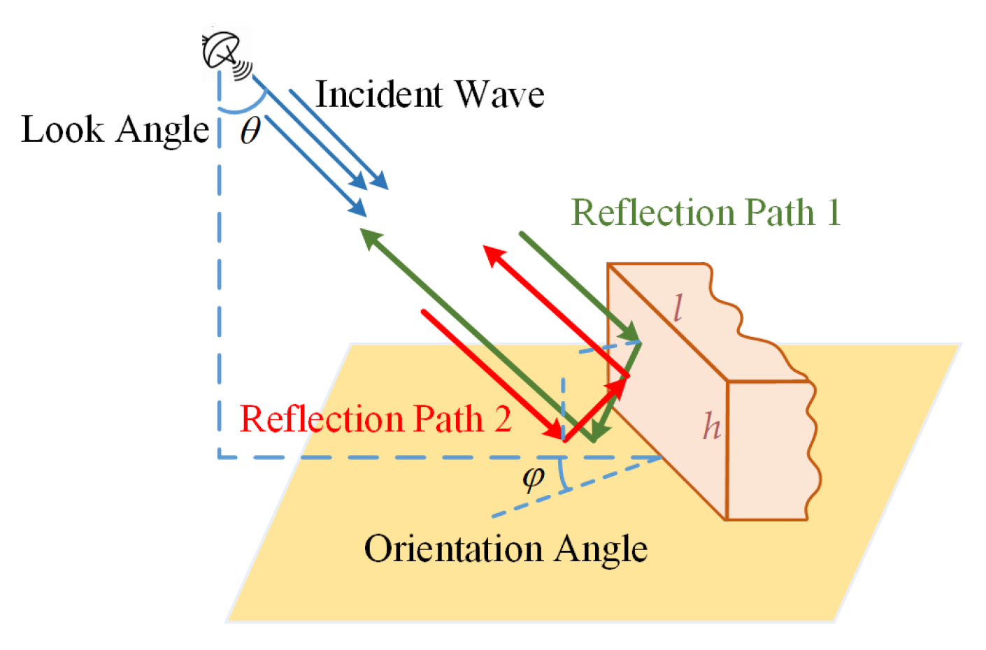
2.1. Scattering Mechanism of Rotational Dihedral

Electromagnetic analysis and calculation are the most accurate way to derive the scattering model. In this paper, a high-frequency approximation technique is chosen to calculate the scattering field and analyze the scattering properties of dihedrals. This is an electromagnetic calculation technique for high-frequency regions that is able to calculate the scattering field of any target. In addition, analytic formulae of the scattering field can be derived that are suitable for the establishment of a basic scattering model [25].

The most commonly used high-frequency approximation methods are PO and GO. PO is able to calculate the far-field scattering while GO can derive the reflection field. By combining these two methods, the scattering field of the dihedral structure can be obtained.

The dihedral scattering analysis model is shown in Figure 1, including a radar system with the look angle of $\theta$ and a dihedral with the orientation angle of $\phi$. According to the analysis and calculation results of the high-frequency approximation method, a double-bounce scattering field dominates the total scattering field when a dihedral exists. Compared with double-bounce scattering, the intensity of surface scattering is very small and can be neglected. Therefore, only two reflection paths are considered in the derivation of a scattering model, namely reflection path 1 (represented by a green line) and reflection path 2 (represented by a red line). Reflection path 1 indicates that the electromagnetic wave is first incident upon the top surface of the dihedral and then reflected to the ground surface. Finally, it is scattered by the ground and received using the radar. Reflection path 2 indicates the wave is first incident on the ground and then reflected to the top surface.

2.2. Derivation of MRDM

The total parametric scattering field of the dihedral can be obtained by calculating the fields of the two reflection paths. The scattering fields of the HH, HV and VV polarization channels are given as follows:

$$\{\begin{array}{c}{E}_{\mathrm{HH}}^s=E_{\mathrm{rP}1\_\mathrm{HH}}^s+E_{\mathrm{rP}2\_\mathrm{HH}}^s\\ E_{\mathrm{HV}}^s=E_{\mathrm{rP}1\_\mathrm{HV}}^s+E_{\mathrm{rP}2\_\mathrm{HV}}^s\\ E_{\mathrm{VV}}^s=E_{\mathrm{rP}1\_\mathrm{VV}}^s+E_{\mathrm{rP}2\_\mathrm{VV}}^s\end{array}$$

(3)

where $E_{\mathrm{rP}1\_\mathrm{HH}}^s,E_{\mathrm{rP}2\_\mathrm{HH}}^s,E_{\mathrm{rP}1\_\mathrm{HV}}^s,E_{\mathrm{rP}2\_\mathrm{HV}}^s,E_{\mathrm{rP}1\_\mathrm{VV}}^s$ and $E_{\mathrm{rP}2\_\mathrm{VV}}^s$ are the scattering fields of each reflection path. The detailed expressions are

$$\begin{array}{c}{E}_{\mathrm{rP}1\_\mathrm{HH}}^s=[2\frac{R_{V1}{\sin }^2\phi -R_{H1}{\cos }^2\theta {\cos }^2\phi }{{\cos }^2\theta +{\sin }^2\theta {\sin }^2\phi }{R}_{H2}\cos \theta \left({\cos }^2\phi -{\sin }^2\phi \right)+\\ 2\frac{\left(R_{H1}+R_{V1}\right)\cos \theta \sin \phi \cos \phi }{{\cos }^2\theta +{\sin }^2\theta {\sin }^2\phi }\sin \phi \cos \phi \left({\sin }^2\theta +R_{V2}+R_{V2}{\cos }^2\theta \right)]\cdot \tan \theta \cos \phi \cdot B\end{array}$$

(4)

$$E_{\mathrm{rP}2\_\mathrm{HH}}^s=\frac{2}{{\cos }^2\theta +{\sin }^2\theta {\sin }^2\phi }\sin \theta \cos \phi \left(R_{H2}{R}_{V1}{\sin }^2\theta {\sin }^2\phi -R_{H1}{R}_{H2}{\cos }^2\theta \right)\cdot B$$

(5)

$$\begin{array}{c}{E}_{\mathrm{rP}1\_\mathrm{HV}}^s=[2\frac{-\left(R_{H1}+R_{V1}\right)\cos \theta \sin \phi \cos \phi }{{\cos }^2\theta +{\sin }^2\theta {\sin }^2\phi }{R}_{V2}\cos \theta \left({\sin }^2\phi -{\cos }^2\phi \right)-\\ 2\frac{R_{V1}{\sin }^2\phi -R_{H1}{\cos }^2\theta {\cos }^2\phi }{{\cos }^2\theta +{\sin }^2\theta {\sin }^2\phi }\sin \phi \cos \phi \left({\sin }^2\theta +R_{H2}+R_{H2}{\cos }^2\theta \right)]\cdot \tan \theta \cos \phi \cdot B\end{array}$$

(6)

$$E_{\mathrm{rP}2\_\mathrm{HV}}^s=-2\frac{\sin \theta \cos \theta \sin \phi }{{\cos }^2\theta +{\sin }^2\theta {\sin }^2\phi }\left[R_{H2}\left({\sin }^2\phi +{\cos }^2\theta {\cos }^2\phi \right)+R_{H1}{R}_{H2}{\sin }^2\theta {\cos }^2\phi +R_{H2}{R}_{V1}\right]\cdot B$$

(7)

$$\begin{array}{c}{E}_{\mathrm{rP}1\_\mathrm{VV}}^s=[2\frac{R_{H1}{\sin }^2\phi -R_{V1}{\cos }^2\theta {\cos }^2\phi }{{\cos }^2\theta +{\sin }^2\theta {\sin }^2\phi }{R}_{V2}\cos \theta \left({\sin }^2\phi -{\cos }^2\phi \right)-\\ 2\frac{\left(R_{H1}+R_{V1}\right)\cos \theta \sin \phi \cos \phi }{{\cos }^2\theta +{\sin }^2\theta {\sin }^2\phi }\sin \phi \cos \phi \left({\sin }^2\theta +R_{H2}+R_{H2}{\cos }^2\theta \right)]\cdot \tan \theta \cos \phi \cdot B\end{array}$$

(8)

$$E_{\mathrm{rP}2\_\mathrm{VV}}^s=\frac{2}{{\cos }^2\theta +{\sin }^2\theta {\sin }^2\phi }\sin \theta \cos \phi \left(R_{V1}{R}_{V2}{\cos }^2\theta -R_{H1}{R}_{V2}{\sin }^2\theta {\sin }^2\phi \right)\cdot B$$

(9)

where $\theta$ is the look angle of the radar, $\phi$ is the orientation angle of the dihedral and $B$ is the phase integral term derived via the Gordon integral algorithm [26]. The detailed form of $B$ is

$$\begin{array}{c}B=-\frac{h\exp \left(jkR\right)}{8\pi R\sin \theta \sin \phi }\cdot [\exp \left(-jk\sin \theta \sin \phi \left(h\tan \theta \sin \phi -l\right)\right)\\ \cdot \sin \mathrm{c}\left(kh\sin \theta \tan \theta {\sin }^2\phi \right)-\exp \left(-jkl\sin \theta \sin \phi \right)]\end{array}$$

(10)

where $k$ is the wave number and $h$ and $l$ are the height and length of the dihedral, respectively. In view of the real look angle of the SAR system, only the parametric model when the look angle is smaller than ${45}^{\circ }$ is presented. The look angle of the proposed MRDM only varies from $0^{\circ }$ to ${45}^{\circ }$. $R_{H1}$ and $R_{V1}$ are the Fresnel reflection coefficients of the top surface, $R_{H2}$ and $R_{V2}$ are those of the ground surface. The Fresnel reflection +coefficients can be defined as [2,27]

$$\begin{array}{l}{R}_H=\frac{\cos {\theta }_l-\sqrt{{\epsilon }_r-{\sin }^2{\theta }_l}}{\cos {\theta }_l+\sqrt{{\epsilon }_r-{\sin }^2{\theta }_l}}\\ R_V=\frac{{\epsilon }_r\cos {\theta }_l-\sqrt{{\epsilon }_r-{\sin }^2{\theta }_l}}{{\epsilon }_r\cos {\theta }_l+\sqrt{{\epsilon }_r-{\sin }^2{\theta }_l}}\end{array}$$

(11)

where ${\epsilon }_r$ is the complex relative permittivity and ${\theta }_l$ is the local incidence angle.

The establishment of a useful dihedral scattering matrix for polarimetric decomposition requires analysis of the scattering field correlation between different polarization channels. However, the scattering fields given in (4)–(9) are too complex to directly derive the polarimetric decomposition model. Therefore, appropriate assumptions need to be made to simplify the model. Based on electromagnetic theory and the Fresnel reflection coefficient calculation principle, it is assumed that $R_{H1}=-R_{V1}$ and $R_{H2}=-R_{V2}$.

Subsequently, the electromagnetic parametric model can be simplified as

$$\{\begin{array}{cc}\hfill E_{\mathrm{HH}}^s=& -4R_{H1}{R}_{H2}\sin \theta {\cos }^3\phi \cdot B\hfill \\ \hfill E_{\mathrm{HV}}^s=& [2R_{H1}\tan \theta \sin \phi {\cos }^2\phi \left({\sin }^2\theta +R_{H2}+R_{H2}{\cos }^2\theta \right)\hfill \\ & -2R_{H2}\sin \theta \cos \theta \sin \phi \left(1-R_{H1}\right)]\cdot B\hfill \\ \hfill E_{\mathrm{VV}}^s=& 4R_{H1}{R}_{H2}\sin \theta {\cos }^3\phi \cdot B\hfill \end{array}$$

(12)

where $\theta$ still lies between $0^{\circ }$ and ${45}^{\circ }$.

After removing the common term, the scattering matrix of MRDM can be expressed as

$$S_d=\left[\begin{array}{cc}-R_{H1}{R}_{H2}& N{R}_{H1}+Q{R}_{H2}+P{R}_{H1}{R}_{H2}\\ N{R}_{H1}+Q{R}_{H2}+P{R}_{H1}{R}_{H2}& R_{H1}{R}_{H2}\end{array}\right]$$

(13)

where

$$N=\frac{1}{2}\tan \theta \sin \theta \tan \phi$$

(14)

$$Q=-\frac{1}{2}\cos \theta \frac{\sin \phi }{{\cos }^3\phi }$$

(15)

$$P=\frac{1}{2}\sin \phi \left(\frac{1}{\cos \theta \cos \phi }+\frac{\cos \theta }{\cos \phi }+\frac{\cos \theta }{{\cos }^3\phi }\right)$$

(16)

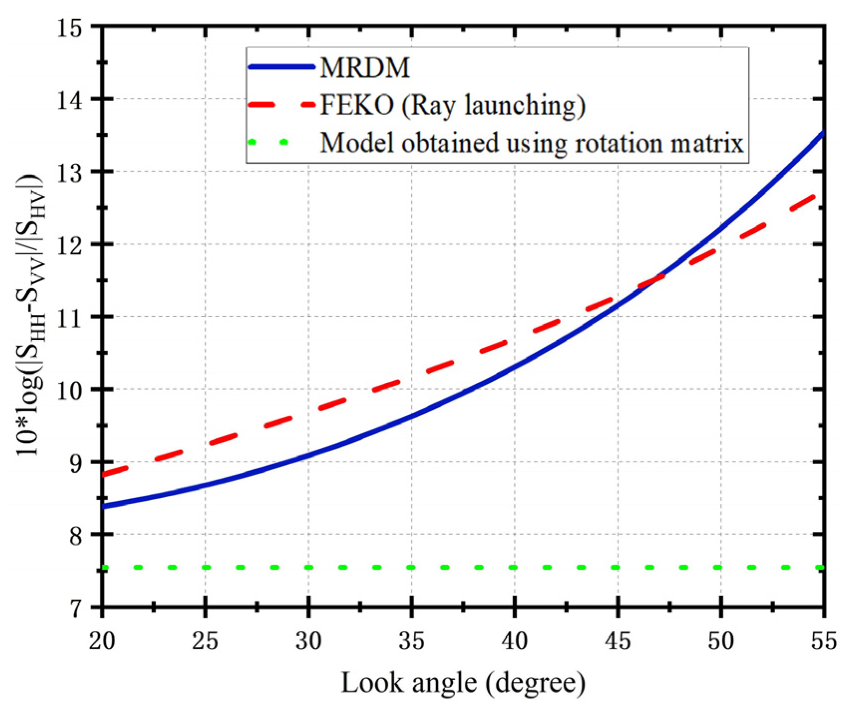
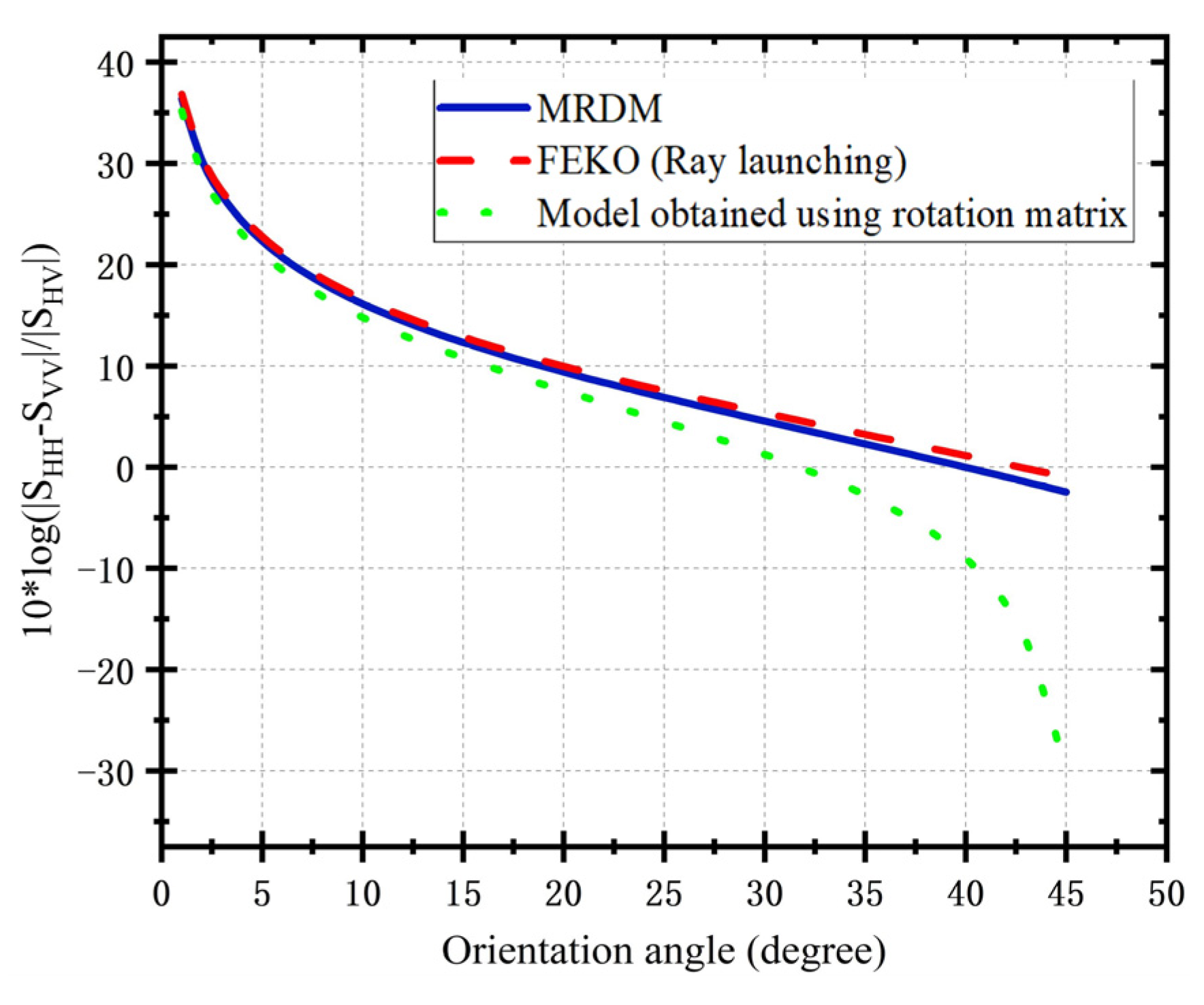
2.3. Precision Analysis of MRDM

In this section, the accuracy of MRDM is verified. A dihedral model with length of 5 m is established for calculation. The frequency of the incident wave is 1.3 GHz (L-Band).

As the model for polarimetric decomposition represents the relationship between various polarization channels, the ratio of $\left|S_{\mathrm{HH}}-S_{\mathrm{VV}}\right|$ to $\left|S_{\mathrm{HV}}\right|$ is selected for comparison and verification. We compare the ratio obtained via MRDM with that calculated via the ray launching technique of Altair FEKO, which is an advanced commercial electromagnetic calculation software [28]. The size of the dihedral is included in the phase integral term $B$, which has no effect on the result of the ratio. In addition to the results of electromagnetic calculation, the traditional dihedral model obtained using the rotation matrix is also compared.

MRDM is proposed with the assumption of $R_{H1}=-R_{V1}$ and $R_{H2}=-R_{V2}$. This assumption introduces some error. However, by comparing the ratios calculated using MRDM under various conditions with those obtained by FEKO, the error is shown to be within acceptable range.

Firstly, the relationship between relative permittivity and the parametric model is investigated. The complex relative permittivity is calculated by

$${\epsilon }_r={{\epsilon }^{\prime }}_r-j\frac{\sigma }{\omega {\epsilon }_0}$$

(17)

where ${{\epsilon }^{\prime }}_r$ is relative permittivity, $\sigma$ is conductivity, $\omega$ is angular frequency and ${\epsilon }_0$ is the permittivity of vacuum. The look angle of the radar is ${33}^{\circ }$ and the orientation angle of the dihedral is ${10}^{\circ }$. The conductivity is fixed to ${10}^{-3}$ $S/m$ and the relative permittivity of the dihedral varies from 1 to 50 with an interval of 0.5. The comparison result is shown in Figure 2. In addition, the ratio under different conductivities is also calculated. The relative permittivity is fixed to 7 and the conductivity varies from ${10}^{-7} S/m$ to ${10}^7 S/m$. The result is shown in Figure 3.

When the relative permittivity is small, the ratios of MRDM have some error compared to the electromagnetic calculation results obtained via FEKO. As the relative permittivity increases, the error decreases gradually. It is worth noting that the ratio of the dihedral model obtained via rotation matrix is constant. It indicates an obvious error in comparison to the electromagnetic calculation result. The results under different conductivities show that there are some errors between MRDM and FEKO results when the conductivities are small. When it becomes large, the error of MRDM is greatly reduced. However, compared with the results obtained via rotation matrix, the precision of MRDM is obviously higher.

The effect of look angle on the accuracy of the model is investigated as well. The orientation angle, relative permittivity and conductivity are set to ${20}^{\circ }$, 7 and ${10}^{-3} S/m$, respectively. The look angle varies from ${20}^{\circ }$ to ${55}^{\circ }$ with an interval of $1^{\circ }$. The comparison graph is shown in Figure 4.

The ratio of the model obtained via rotation matrix is still a constant, since there is no look angle parameter in the model. Therefore, there is a generous error compared with the electromagnetic calculation result. The result of MRDM is closer to that of electromagnetic calculation in the overall trend, which better describes the scattering mechanism of rotational dihedral structure.

Finally, the influence of orientation angle is analyzed. The look angle, relative permittivity and conductivity are set to ${33}^{\circ }$, 7 and ${10}^{-3} S/m$. The orientation angle of the dihedral varies from $1^{\circ }$ to ${45}^{\circ }$ with an interval of $1^{\circ }$. The ratios of different models are shown in Figure 5.

It can be seen that the error of MRDM is smaller than the model obtained via rotation matrix. When the orientation angle is large, the error of model given by the rotation matrix increases gradually. However, MRDM can still characterize the scattering property of dihedrals accurately.

On the basis of these results, it can be concluded that MRDM can better describe the polarized scattering mechanism of rotational dihedrals. Although the approximation will introduce error, MRDM still has higher accuracy compared with the dihedral model obtained via rotation matrix, especially it describes the impact of look angle and relative permittivity more accurately.

2.4. The Coherency Matrix of MRDM

In order to apply MRDM to the decomposition method, the model needs to be transformed to the form of coherency matrix $T$ first. According to (13), the coherency matrix of MRDM is

$$T_d=\left[\begin{array}{ccc}0& 0& 0\\ 0& 2{\left|R_{H1}{R}_{H2}\right|}^2& -R_{H1}{R}_{H2}{M}^{\ast }\\ 0& -R_{H1}^{\ast }{R}_{H2}^{\ast }M& 2{\left|N{R}_{H1}+Q{R}_{H2}+P{R}_{H1}{R}_{H2}\right|}^2\end{array}\right]$$

(18)

where

$$M=N{R}_{H1}+Q{R}_{H2}+P{R}_{H1}{R}_{H2}$$

(19)

In order to set up the decomposition equation, the model is transformed into

$$T_d=f_d\left[\begin{array}{ccc}0& 0& 0\\ 0& 2& -\left({\alpha }^{\ast }+P\right)\\ 0& -\left(\alpha +P\right)& 2{\left|\alpha +P\right|}^2\end{array}\right]$$

(20)

where

$$f_d={\left|R_{H1}{R}_{H2}\right|}^2$$

(21)

$$\alpha =\frac{R_{H2}^{\ast }}{{\left|R_{H2}\right|}^2}N+\frac{R_{H1}^{\ast }}{{\left|R_{H1}\right|}^2}Q$$

(22)

It can be seen from the coherency matrix that the main energy comes from $T_{22},T_{23},T_{32}$ and $T_{33}$. This is caused by the assumptions when we try to simplify the scattering model. However, when the orientation angle of the urban area is small, the energy of the dihedral induced by $T_{11},T_{12},T_{21}$ and $T_{22}$ is still considerable. Therefore, the modified rotational dihedral model is more suitable for decomposition in urban areas with certain orientation angles. For the urban areas with very small orientation angle, it is possible to cause the overestimation of other scattering components except dihedral components. In this case, the current image region is classified based on the estimated orientation angle. For a region with small orientation angle, the traditional $0^{\circ }$-oriented dihedral scattering model is used for polarimetric decomposition. For a region with large orientation angle, MRDM is used.

3. Five-component Scattering Decomposition

In this section, MRDM is applied to PolSAR images by introducing it to a five-component scattering decomposition method (MRDM-5SD). The process of MRDM-5SD is mainly divided into orientation angle estimation and solutions of scattering contributions.

3.1. Orientation Angle Estimation

Orientation angle estimation is a necessary prerequisite step of the proposed decomposition method. In previous studies [19,29], some estimation methods of orientation angle have been proposed. However, the range of the angle is limited within $\pm {45}^{\circ }$. Based on the theory of scattering similarity [30], a new orientation angle estimation method is proposed. The range of the estimated angle is extended to $\pm {90}^{\circ }$, which is conductive to the distinction between the urban and vegetation areas in the proposed decomposition method.

First, an orientation angle estimation matrix derived from MRDM is given as follows:

$$P_{\phi }=\left[\begin{array}{cc}-{\cos }^3\phi & \cos \theta \sin \phi \left(1+{\cos }^2\phi \right)\\ \cos \theta \sin \phi \left(1+{\cos }^2\phi \right)& {\cos }^3\phi \end{array}\right]$$

(23)

According to the theory of scattering similarity, the polarimetric similarity between measured data and the orientation angle estimation matrix can be calculated using [30].

$$r\left(\phi \right)=\frac{k_{\phi }^{\mathrm{H}}\langle T\rangle k_{\phi }}{\mathrm{Trace}\left(k_{\phi }\cdot k_{\phi }^{\mathrm{H}}\right)\cdot \mathrm{Trace}\left(\langle T\rangle \right)}$$

(24)

where the superscript H means conjugate transpose, $T$ is the coherency matrix, and $k_{\phi }$ is the Pauli vector of $P_{\phi }$, $\mathrm{Trace}(\cdot )$ denotes the trace operation of the matrix and $\langle \cdot \rangle$ is the ensemble average in an imaging window.

The estimated orientation angle is obtained by cycling through the angle within the range of $\pm {90}^{\circ }$ and calculating the similarity coefficients. When the similarity coefficient reaches maximum, output the angle as estimated orientation angle:

$${\phi }_{\mathrm{estimated}}=\underset{\phi }{\arg \max r\left(\phi \right)}\hspace{0.17em}\hspace{0.17em}\hspace{0.17em},\hspace{0.17em}\hspace{0.17em}\hspace{0.17em}\phi \in \left(-{90}^{\circ },{90}^{\circ }\right)\hspace{0.17em}\hspace{0.17em}\hspace{0.17em}\hspace{0.17em}$$

(25)

3.2. Five-component Scattering Decomposition (MRDM-5SD)

Based on the orientation angle estimation and MRDM, MRDM-5SD is proposed. According to the scattering mechanism analysis of oriented buildings and other observed areas, five scattering components are included in the decomposition method, namely surface scattering, modified rotational dihedral scattering (derived via MRDM), volume scattering, $\pm {45}^{\circ }$ oriented dipole scattering and compound dipole scattering. The latter two dipole scattering components come from the 6SD decomposition method [20].

According to estimated orientation angle, two cases for polarimetric decomposition can be listed as follows:

$$\begin{array}{l}\mathrm{case}\hspace{0.17em}1:\hspace{0.17em}\hspace{0.17em}\langle T\rangle =f_s{T}_S+f_d{T}_{D1}+f_v{T}_V+f_{od}{T}_{OD}+f_{cd}{T}_{CD}\\ \hspace{0.17em}\hspace{0.17em}\hspace{0.17em}\hspace{0.17em}\hspace{0.17em}\hspace{0.17em}\hspace{0.17em}\hspace{0.17em}\hspace{0.17em}\hspace{0.17em}\hspace{0.17em}=f_s\left[\begin{array}{ccc}1& {\beta }^{\ast }& 0\\ \beta & {\left|\beta \right|}^2& 0\\ 0& 0& 0\end{array}\right]+f_d\left[\begin{array}{ccc}{\left|{\alpha }_1\right|}^2& {\alpha }_1& 0\\ {\alpha }_1{}^{\ast }& 1& 0\\ 0& 0& 0\end{array}\right]+\frac{f_v}{4}\left[\begin{array}{ccc}2& 0& 0\\ 0& 1& 0\\ 0& 0& 1\end{array}\right]+\hspace{0.17em}\max \left(\frac{f_{od}}{2}\left[\begin{array}{ccc}1& 0& \pm 1\\ 0& 0& 0\\ \pm 1& 0& 1\end{array}\right]+\frac{f_{cd}}{2}\left[\begin{array}{ccc}1& 0& \pm j\\ 0& 0& 0\\ \pm j& 0& 1\end{array}\right]\right)\end{array}$$

(26)

$$\begin{array}{l}\mathrm{case}2:\hspace{0.17em}\langle T\rangle =f_s{T}_S+f_d{T}_{D2}+f_v{T}_V+f_{od}{T}_{OD}+f_{cd}{T}_{CD}\\ \hspace{0.17em}\hspace{0.17em}\hspace{0.17em}\hspace{0.17em}\hspace{0.17em}\hspace{0.17em}\hspace{0.17em}\hspace{0.17em}=f_s\left[\begin{array}{ccc}1& {\beta }^{\ast }& 0\\ \beta & {\left|\beta \right|}^2& 0\\ 0& 0& 0\end{array}\right]+f_d\left[\begin{array}{ccc}0& 0& 0\\ 0& 2& -\left({\alpha }_2{}^{\ast }+P\right)\\ 0& -\left({\alpha }_2+P\right)& 2{\left|{\alpha }_2+P\right|}^2\end{array}\right]+\hspace{0.17em}\frac{f_v}{4}\left[\begin{array}{ccc}2& 0& 0\\ 0& 1& 0\\ 0& 0& 1\end{array}\right]+\hspace{0.17em}\hspace{0.17em}\max \left(\frac{f_{od}}{2}\left[\begin{array}{ccc}1& 0& \pm 1\\ 0& 0& 0\\ \pm 1& 0& 1\end{array}\right]+\frac{f_{cd}}{2}\left[\begin{array}{ccc}1& 0& \pm j\\ 0& 0& 0\\ \pm j& 0& 1\end{array}\right]\right)\end{array}$$

(27)

Case 1 is mainly for flat ground surfaces, water surfaces and urban areas with small orientation angles. It is important to note that only the higher energy of the two dipole scattering components is kept, which ensures that the remaining scattering components produce as little negative energy as possible. Case 2 is for urban areas with large orientation angles or random scattering areas such as vegetation, in which MRDM is used. $f_s,f_d,f_v,f_{od}$ and $f_{cd}$ are scattering coefficients corresponding to surface scattering, double-bounce scattering, volume scattering, $\pm {45}^{\circ }$ oriented dipole scattering and compound dipole scattering, respectively. $T_S,T_{D1}\hspace{0.17em}\mathrm{or}\hspace{0.17em}{T}_{D2},T_V,T_{OD}$ and $T_{CD}$ are the scattering models corresponding to them; ${\alpha }_1,{\alpha }_2$ and $\beta$ are unknowns that need to be determined.

Based on the two cases, the contribution of each scattering component can be calculated using

$$\{\begin{array}{l}{P}_s=f_s\left(1+{\left|\beta \right|}^2\right)\hfill \\ P_d=f_d\left(1+{\left|{\alpha }_1\right|}^2\right)\hspace{0.17em}\hspace{0.17em}or\hspace{0.17em}\hspace{0.17em}{P}_d=2f_d\left(1+{\left|{\alpha }_2+P\right|}^2\right)\hfill \\ P_v=f_v\hfill \\ P_{od}=f_{od}\hfill \\ P_{cd}=f_{cd}\hfill \end{array}$$

(28)

where $P_s,P_d,P_v,P_{od}$ and $P_{cd}$ are the contribution of surface scattering, double-bounce scattering, volume scattering, $\pm {45}^{\circ }$ oriented dipole scattering and compound dipole scattering, respectively.

3.3. Branch Conditions and Flowchart of MRDM-5SD

In order to determine which case to use, the variance ${\phi }_{\mathrm{var}}$ and the mean value ${\phi }_{\mathrm{mean}}$ of the orientation angles in an imaging window are used for scattering mechanism discrimination. According to Figure 5, when the orientation angle is small, the dihedral model obtained via rotation matrix shows higher accuracy. In the remaining cases, MRDM has higher accuracy. Therefore, the cases are chosen according to the following conditions:

$$\begin{array}{l}{\phi }_{\mathrm{var}}<\mathrm{VarB}\hspace{0.17em}\hspace{0.17em}and\hspace{0.17em}\left|{\phi }_{\mathrm{mean}}\right|<5^{\circ }\hspace{0.17em}\hspace{0.17em}\to \hspace{0.17em}\hspace{0.17em}Case\hspace{0.17em}1\\ \hspace{0.17em}\hspace{0.17em}\hspace{0.17em}\hspace{0.17em}\left(\mathrm{Small} \mathrm{oriented} \mathrm{urban} \mathrm{area}, \mathrm{Flat} \mathrm{ground}, \mathrm{Water} \mathrm{surface}\right)\\ {\phi }_{\mathrm{var}}\ge \mathrm{VarB}\hspace{0.17em}\hspace{0.17em}or\hspace{0.17em}\left|{\phi }_{\mathrm{mean}}\right|>5^{\circ }\hspace{0.17em}\hspace{0.17em}\to \hspace{0.17em}\hspace{0.17em}Case\hspace{0.17em}2\\ \hspace{0.17em}\hspace{0.17em}\hspace{0.17em}\hspace{0.17em}\left(\mathrm{Highly} \mathrm{oriented} \mathrm{urban} \mathrm{area}, \mathrm{Random} \mathrm{scattering}\right)\end{array}$$

(29)

where $\mathrm{VarB}$ is a threshold value. When $\left|{\phi }_{\mathrm{mean}}\right|$ is smaller than $5^{\circ }$, the current area is considered to be a flat area or small oriented urban area. Otherwise, it is considered to be highly oriented urban area. $\mathrm{VarB}$ is used to determine the vegetation area, which is chosen according to the degree of orientation angle dispersion in random scattering areas.

When case 1 is chosen, a more detailed scattering mechanism needs to be discriminated. There are three equations with four unknowns, which means that one of the unknowns needs to be fixed to acquire the solution. According to [31], when $\langle T_{11}\rangle -\langle T_{22}\rangle >0$, surface scattering is the dominant scattering mechanism. In this case, we can assume ${\alpha }_1=0$. Otherwise, double-bounce scattering is dominant and $\beta$ is fixed to zero. Under the assumption, the equation of case 1 can be solved.

For case 2, the number of equations is equal to the unknowns, so no assumptions need to be made. First, the dihedral scattering coefficient $f_d$ is solved. It is worth mentioning that a cubic equation needs to be solved to obtain $f_d$. The equation may have one, two or three solutions. When the equation has multiple solutions, it is necessary to determine which solution to choose according to the scattering mechanism of the current region. When the variance of the orientation angle is less than the threshold $\mathrm{VarB}$, the change in the orientation angle in this area is not drastic, which means that it can be an urban area. In this case, the largest solution is taken as $f_d$. Otherwise, random scattering is considered to be the dominant scattering mechanism of this region, so the smallest solution is taken.

By using the branch conditions, all the equations can be solved and the contribution of each scattering component can be obtained. The flow chart of MRDM-5SD is illustrated in Figure 6.

3.4. Solutions of MRDM-5SD

In this section, the detailed solutions for MRDM-5SD are given. The contribution of the two dipole scattering components can be directly calculated via

$$\begin{array}{c}{f}_{od}=2\left|\mathrm{real}\left(\langle T_{13}\rangle \right)\right|\\ f_{cd}=2\left|\mathrm{imag}\left(\langle T_{13}\rangle \right)\right|\end{array}$$

(30)

Only the larger contribution of the two-dipole scattering remains, and the other contribution is fixed to zero. Then the coherency matrix can be updated using

$$\begin{array}{l}\langle T_{11}\rangle =\langle T_{11}\rangle -\max \left(f_{od}/2,f_{cd}/2\right)\\ \langle T_{33}\rangle =\langle T_{33}\rangle -\max \left(f_{od}/2,f_{cd}/2\right)\end{array}$$

(31)

For case 1, the solution has been given by Freeman-Durden [14] and Singh. [20], which can be summarized as

$$\begin{array}{cc}\begin{array}{l}\langle T_{11}\rangle -\langle T_{22}\rangle >0:\\ \{\begin{array}{l}\alpha =0\hfill \\ f_v=4\langle T_{33}\rangle \hfill \\ f_s=\langle T_{11}\rangle -f_v/2\hspace{0.17em}\hspace{0.17em}\hspace{0.17em}\hspace{0.17em}\hspace{0.17em}\hspace{0.17em}\hspace{0.17em}\hspace{0.17em}\hspace{0.17em}\hspace{0.17em}\hspace{0.17em}or\hfill \\ \beta =\langle T_{21}\rangle /f_s\hfill \\ f_d=\langle T_{22}\rangle -f_v/4-f_s{\left|\beta \right|}^2\hfill \end{array}\hspace{0.17em}\end{array}& \begin{array}{l}\langle T_{11}\rangle -\langle T_{22}\rangle \le 0:\hspace{0.17em}\hspace{0.17em}\hspace{0.17em}\hspace{0.17em}\hspace{0.17em}\hspace{0.17em}\hspace{0.17em}\hspace{0.17em}\hspace{0.17em}\hspace{0.17em}\hspace{0.17em}\hspace{0.17em}\hspace{0.17em}\hspace{0.17em}\hspace{0.17em}\\ \{\begin{array}{l}\beta =0\hfill \\ f_v=4\langle T_{33}\rangle \hfill \\ f_d=\langle T_{22}\rangle -f_v/4\hfill \\ \alpha =\langle T_{21}\rangle /f_d\hfill \\ f_s=\langle T_{11}\rangle -f_v/2-f_d{\left|\alpha \right|}^2\hfill \end{array}\end{array}\end{array}$$

(32)

Then the contribution of each scattering component can be calculated using (28). For case 2, five equations can be formed:

$$\{\begin{array}{l}{f}_s+\frac{f_v}{2}=\langle T_{11}\rangle \hfill \\ \beta f_s=\langle T_{21}\rangle \hfill \\ f_s{\left|\beta \right|}^2+2f_d+\frac{f_v}{4}=\langle T_{22}\rangle \hfill \\ -f_d\left({\alpha }_2+P\right)=\langle T_{32}\rangle \hfill \\ \frac{f_v}{4}+2f_d{\left|\alpha +P\right|}^2=\langle T_{33}\rangle \hfill \end{array}$$

(33)

After eliminating the remaining unknowns, a cubic equation of $f_d$ can be given as

$$a{f}_d^3+b{f}_d^2+c{f}_d+d=0$$

(34)

where

$$\begin{array}{l}a=4\langle T_{11}\rangle -8\langle T_{33}\rangle \\ b=2{\left|\langle T_{21}\rangle \right|}^2+16{\left|\langle T_{32}\rangle \right|}^2+2\langle T_{11}\rangle \langle T_{33}\rangle -2\langle T_{11}\rangle \langle T_{22}\rangle +4\langle T_{22}\rangle \langle T_{33}\rangle -4{\langle T_{33}\rangle }^2\\ c=16{\left|\langle T_{32}\rangle \right|}^2\langle T_{33}\rangle -8{\left|\langle T_{32}\rangle \right|}^2\langle T_{22}\rangle -4{\left|\langle T_{32}\rangle \right|}^2\langle T_{11}\rangle \\ d=-16{\left|\langle T_{32}\rangle \right|}^4\end{array}$$

(35)

Once $f_d$ is solved, other coefficients can be calculated via

$$\{\begin{array}{l}{f}_v=4\left(\langle T_{33}\rangle -\frac{2{\left|\langle T_{32}\rangle \right|}^2}{f_d}\right)\hfill \\ f_s=\langle T_{11}\rangle -f_v/2\hfill \\ \beta =\langle T_{21}\rangle /f_s\hfill \\ {\alpha }_2+P=-\langle T_{32}\rangle /f_d\hfill \end{array}$$

(36)

Finally, the contribution can also be calculated via (28).

4. Experimental Results and Discussion

In this section, three fully polarimetric data sets are used to verify the proposed five-component decomposition method, which are listed in

Table 1. List of fully polarimetric data sets.

(37)	Carrier	Band	Resolution (Azimuth × Range)	Area	Ground Objects	Acquisition Data
ALOS-2/ PALSAR-2	Spaceborne	L	3.20 m $\times$ 2.86 m	San Francisco, USA	Water, hills, urban area	2015/3/24
GF-3	Spaceborne	C	8 m $\times$ 8 m	Harbin, China	Water, farmland, urban area	2017/7/23
E-SAR	Airborne	L	3 m $\times$ 2.2 m	Oberpfaffenhofen, Germany	Vegetation, grass land, urban area, airport	2022/8/26

. Data sets acquired by both airborne and spaceborne sensors of different bands are used. The spatial window size for calculation of coherency matrix is $3\times 3$ in all experiments. The existing decomposition methods Y4O, Y4R, G4U, 6SD and 7SD are compared with MRDM-5SD. The scattering mechanism contributions in several patches decomposed using these methods are presented and analyzed.

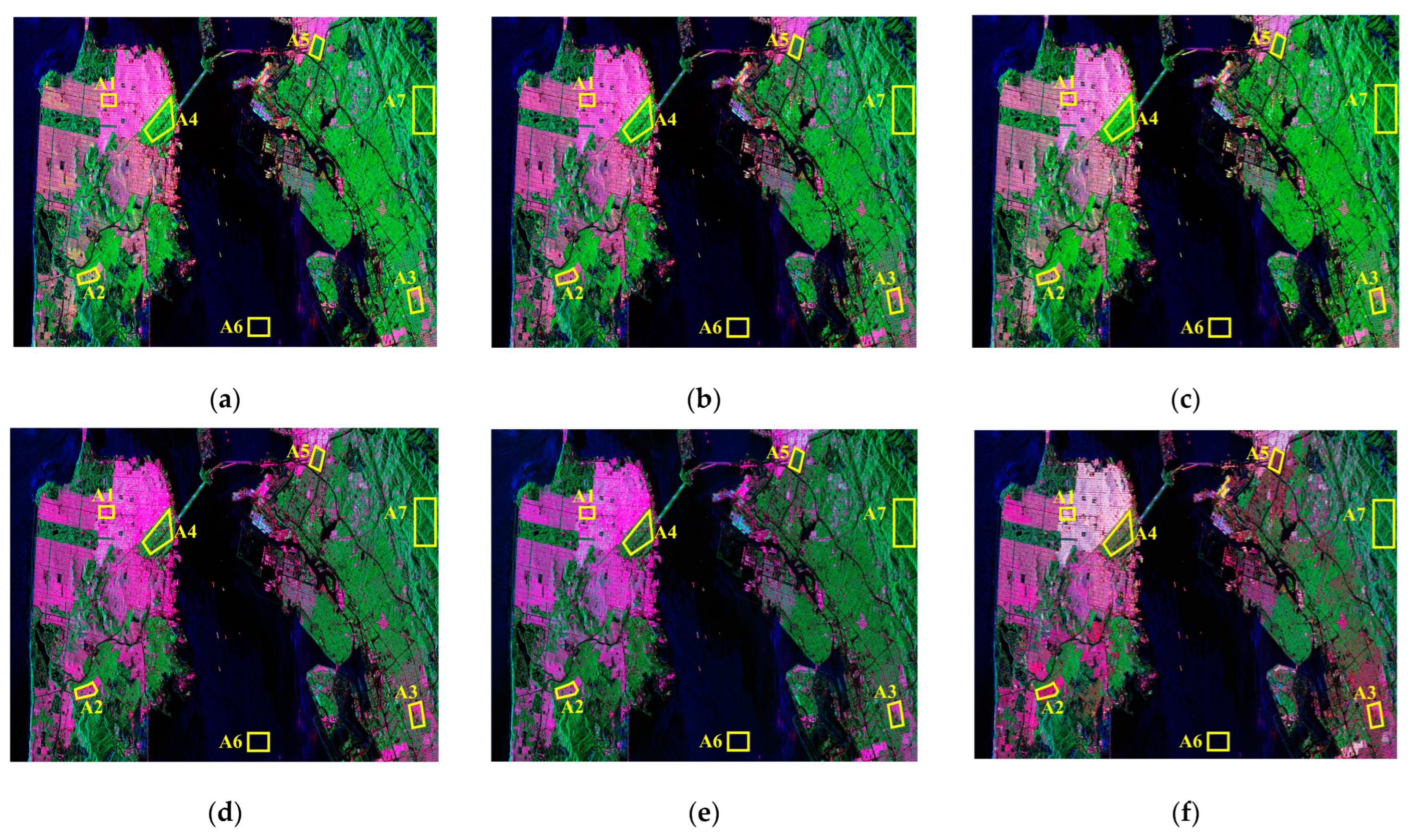
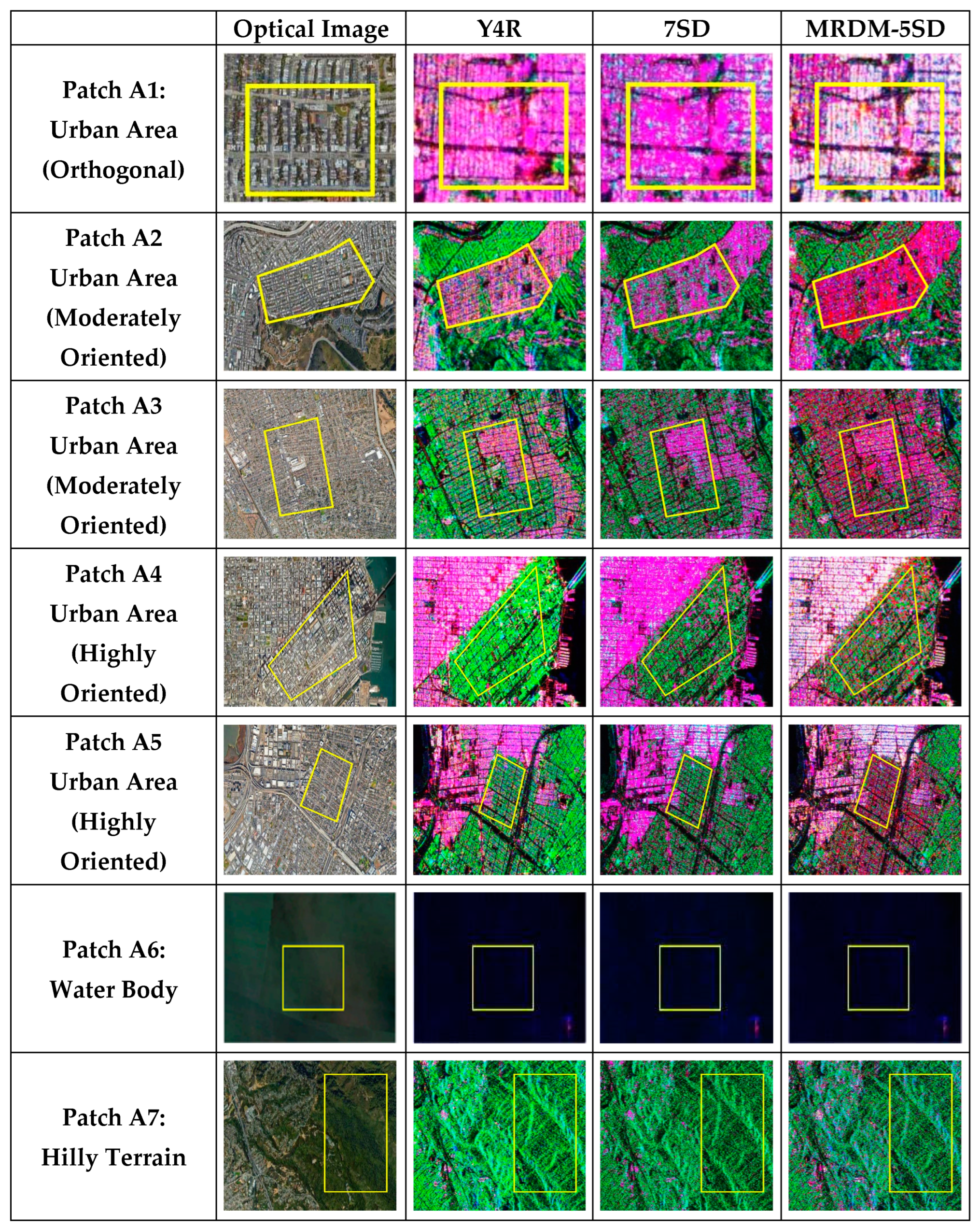
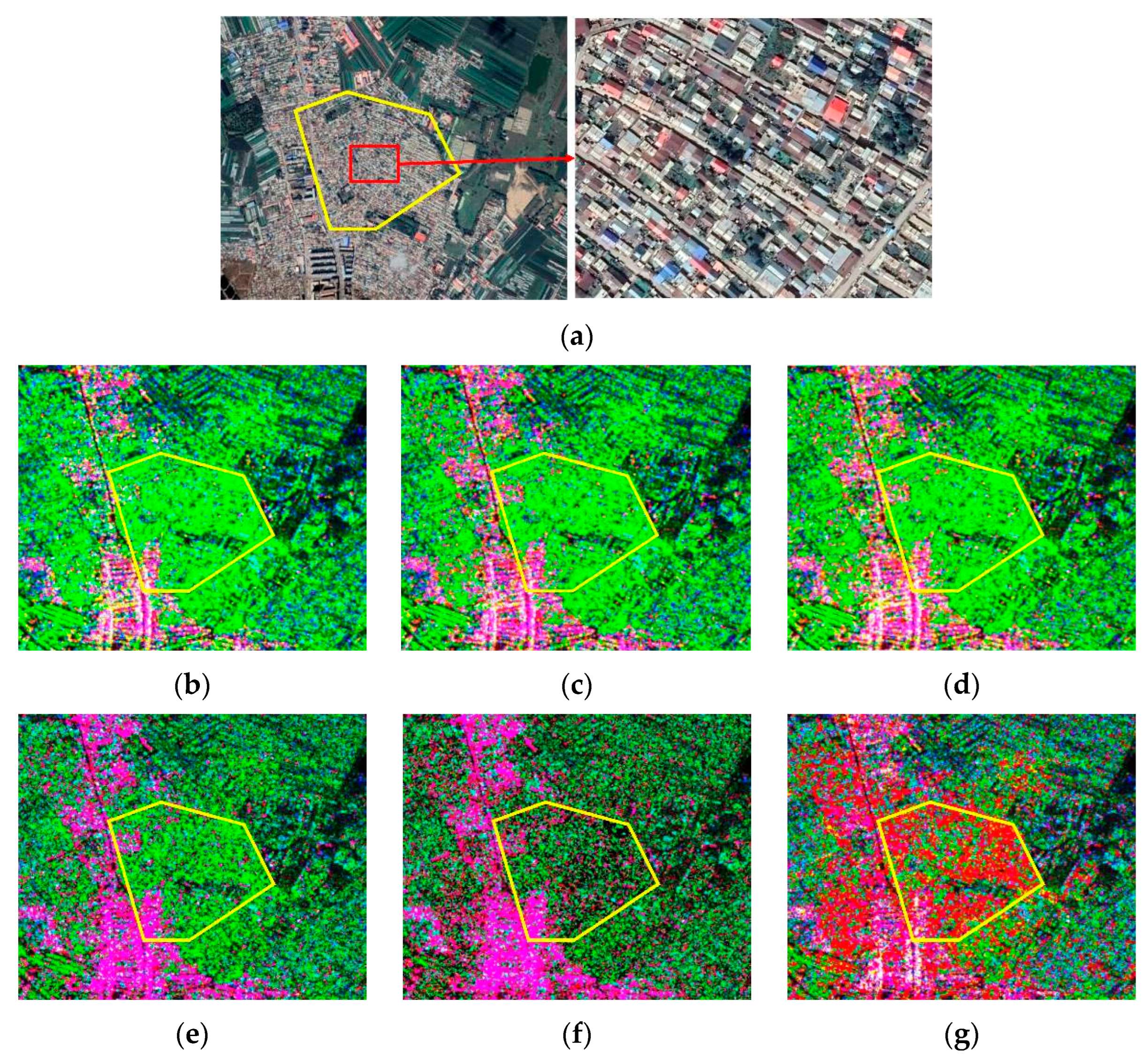
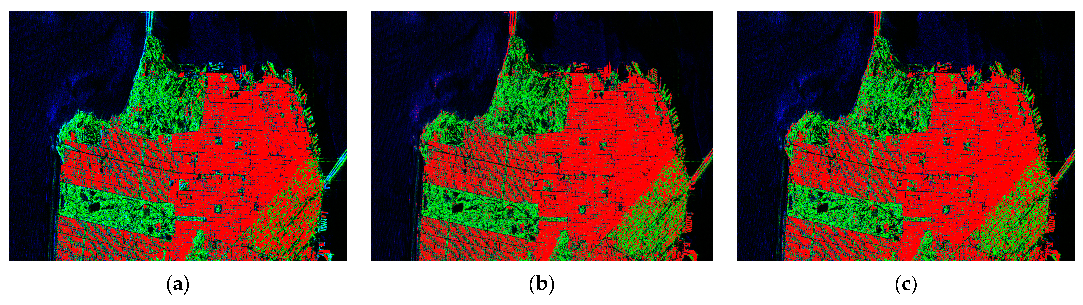
4.1. Validation by Spaceborne ALOS-2/PALSAR-2 Datasets

Data sets from spaceborne ALOS-2/PALSAR-2 over the city of San Francisco, CA, USA were used to verify the proposed method, and include water body, hills and urban areas with various orientation angles. The optical image from Google Earth is shown in Figure 7.

The orientation angle estimation result is shown in Figure 8, which is an essential step in the proposed method. Seven regions of interest (ROIs) are selected to analyze the estimated orientation angles. Patch A1 and A6 are orthogonal urban area and water area, whose orientation angles tend to $0^{\circ }$. Patch A2 and A3 are moderately oriented urban areas and the orientation angles are around ${20}^{\circ }$. Patch A4 and A5 are highly oriented urban areas. However, due to the different rotation directions, the angles are positive and negative, respectively. Patch A7 is hilly terrain and the estimated orientation angles are disordered.

The decomposition results of Y4O, Y4R, G4U, 6SD, 7SD and MRDM-5SD are shown in Figure 9. Y4R introduces the rotation matrix, and thus the contributions of double-bounce scattering are improved in some urban areas compared with Y4O. However, volume scattering is still dominant in urban areas with large orientation angles. A similar phenomenon can also be observed in the result of G4U. Compared with other methods, the double-bounce scattering contributions in urban areas with moderate orientation angle are improved obviously in the results of 6SD and 7SD. Nevertheless, in urban areas with large orientation angles, the results are still not satisfying. MRDM-5SD is able to further improve the decomposition results, increasing the percentages of double-bounce scattering in most urban areas.

To further confirm the validity of the proposed decomposition method, the detailed scattering contributions of Patch A1-A7 were calculated. The enlarged view of Y4R, 7SD and MRDM-5SD is shown in Figure 10 and scattering contributions of all methods are listed in

Table 2. Scattering contributions (%) of Patch A1-A7 for ALOS-2/PALSAR-2 data sets.

ROIs	Methods	${\mathit{P}}_{\mathit{s}}$	${\mathit{P}}_{\mathit{d}}$	${\mathit{P}}_{\mathit{v}}$	${\mathit{P}}_{\mathit{h}}$	${\mathit{P}}_{\mathit{o}\mathit{d}}$	${\mathit{P}}_{\mathit{c}\mathit{d}}$	${\mathit{P}}_{\mathit{m}\mathit{d}}$
Patch A1	Y4O	30.6	53.2	12.5	3.7	-	-	-
	Y4R	32.2	56.6	8.7	2.5	-	-	-
	G4U	28.5	57.4	13.9	0.3	-	-	-
	6SD	29.8	59.3	4.2	2.4	2.1	2.3	-
	7SD	29.8	56.7	4.7	1.7	1.4	1.2	4.5
	MRDM-5SD	32.5	57.4	6.2	-	2.0	1.9	-
Patch A2	Y4O	21.5	28.2	42.4	7.9	-	-	-
	Y4R	27.5	52.0	16.3	4.2	-	-	-
	G4U	23.0	53.1	23.5	0.4	-	-	-
	6SD	24.5	57.0	7.7	3.3	3.7	3.8	-
	7SD	21.7	44.1	9.5	1.4	3.7	2.4	17.2
	MRDM-5SD	19.0	65.1	3.5	-	7.5	4.9	-
Patch A3	Y4O	22.1	17.3	49.8	10.8	-	-	-
	Y4R	27.4	29.5	34.5	8.6	-	-	-
	G4U	21.0	32.5	45.8	0.7	-	-	-
	6SD	24.3	37.8	16.3	6.1	7.9	7.6	-
	7SD	19.9	32.0	18.6	4.8	6.3	5.8	12.6
	MRDM-5SD	22.3	50.4	10.7	-	8.6	8.0	-
Patch A4	Y4O	21.0	10.0	57.2	11.8	-	-	-
	Y4R	20.0	13.4	55.7	10.9	-	-	-
	G4U	17.0	15.1	67.7	0.2	-	-	-
	6SD	18.4	22.4	18.3	7.0	16.0	17.9	-
	7SD	19.5	27.0	12.2	6.0	12.7	11.0	11.6
	MRDM-5SD	24.0	42.8	13.2	-	9.2	10.8	-
Patch A5	Y4O	34.3	22.9	35.0	7.8	-	-	-
	Y4R	37.5	31.2	25.1	6.2	-	-	-
	G4U	32.5	33.3	33.7	0.5	-	-	-
	6SD	34.7	37.3	12.8	4.4	5.5	5.3	-
	7SD	32.8	33.6	14.4	3.4	4.1	3.7	8.0
	MRDM-5SD	33.9	45.6	8.8	-	6.3	5.4	-
Patch A6	Y4O	78.2	7.8	8.2	5.8	-	-	-
	Y4R	78.7	8.1	7.7	5.5	-	-	-
	G4U	76.1	8.2	9.3	6.4	-	-	-
	6SD	65.8	7.3	9.1	5.8	6.0	6.0	-
	7SD	82.1	4.4	13.1	0.1	0.1	0.1	0.1
	MRDM-5SD	82.9	8.8	7.1	-	0.6	0.6	-
Patch A7	Y4O	24.0	6.6	58.5	10.9	-	-	-
	Y4R	25.5	10.2	53.7	10.6	-	-	-
	G4U	19.6	13.5	66.0	0.9	-	-	-
	6SD	23.1	18.1	31.7	6.9	10.2	10.0	-
	7SD	20.2	15.9	34.2	5.9	9.0	8.8	6.0
	MRDM-5SD	26.7	22.5	32.0	-	9.5	9.3	-

, where $P_s,P_d,P_v,P_h,P_{od},P_{cd}$ and $P_{md}$ are the scattering contributions of surface scattering, double-bounce scattering, volume scattering, helix scattering, $\pm {45}^{\circ }$ oriented dipole scattering, compound dipole scattering and mixed dipole scattering.

Patch A1 is an area of orthogonal urban area, which is decomposed via the $0^{\circ }$-oriented dihedral scattering model in MRDM-5SD. According to the RGB result of decomposition and the contribution percentages in Table 2, double-bounce scattering is dominant in all decomposition schemes. The area exhibits powerful purple, which is a combination of double-bounce scattering and surface scattering. The detailed percentages of double-bounce scattering are 53.2%, 56.6%, 57.4%, 59.3%, 56.7% and 57.4% for Y4O, Y4R, G4U, 6SD, 7SD and MRDM-5SD, respectively.

For urban areas with moderate orientation angles (Patch A2 and A3), double-bounce scattering is still dominant. However, the proportion decreases significantly, especially in Patch A3. The scattering contribution percentages of dihedrals in MRDM-5SD are 65.1% and 50.4% for Patch A2 and A3, respectively. Obviously, the contribution of dihedral scattering is improved significantly compared with other methods, which can be seen from the enlarged view as well. The red color in the result of MRDM-5SD is more pronounced than in the other decomposition results.

Patch A4 and A5 are urban areas with large orientation angles. There has been a significant decline in the dihedral contribution in most decomposition methods. Volume scattering dominates in decomposition methods such as Y4R and G4U, failing to extract accurate features and exhibiting green. The percentages of double-bounce scattering over Patch A4 are 10.0%, 13.4%, 15.1%, 22.4%, 27.0% and 42.8% in Y4O, Y4R, G4U, 6SD, 7SD and MRDM-5SD, respectively. The contribution of double-bounce scattering can be improved effectively in MRDM-5SD and that of volume scattering can be reduced to some extent. Additionally, there are rooftops and highways in this area, so the percentage of surface scattering is high as well. In Patch A5, the percentage of double-bounce scattering in MRDM-5SD is 45.6%, which is obviously higher than those of other decomposition methods. The volume scattering contribution declines to 8.8%, verifying the effectiveness of MRDM-5SD in urban areas with large orientation angles.

The surface of water body area (Patch A6) is relatively flat, so surface scattering contribution is dominant. The area exhibits blue, which is dark since the scattering power is relatively weak compared with other areas. The detailed percentages of surface scattering are 78.2%, 78.7%, 76.1%, 65.8%, 82.1% and 82.9% for Y4O, Y4R, G4U, 6SD, 7SD and MRDM-5SD, respectively. The effectiveness of the decomposition in areas with flat surface is improved as well by using MRDM-5SD. Patch A7 is an area of hilly terrain with vegetation, where volume scattering contribution is dominant. The percentage of the volume scattering in MRDM-5SD is 32.0%. Additionally, due to the slope of the terrain, the proportion of surface scattering is also considerable. All the data and the enlarged view confirm that MRDM-5SD is also effective in random scattering areas such as forests.

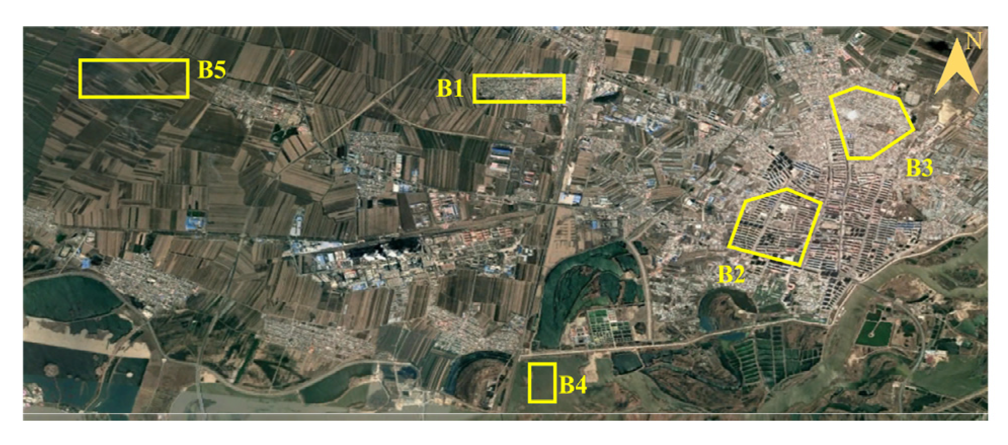
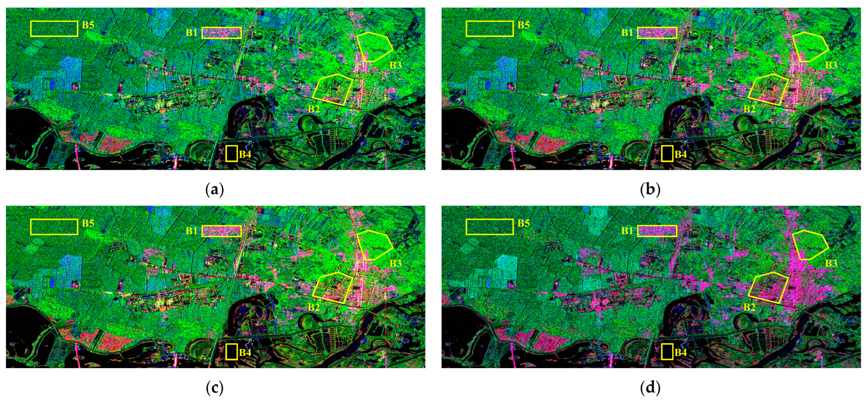
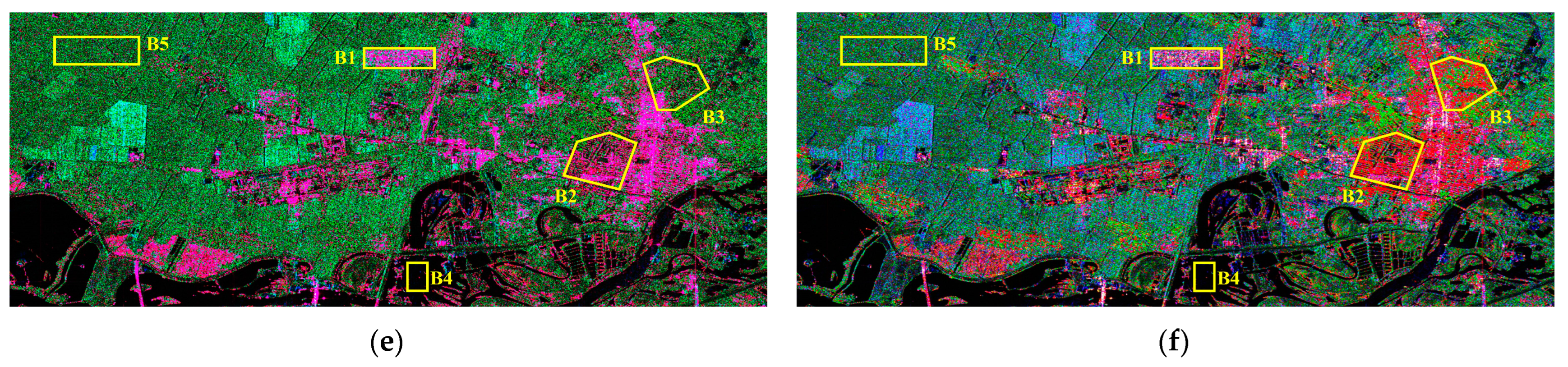
4.2. Validation by Spaceborne GF-3 Datasets

Another data set obtained using GF-3 over the city of Harbin, China was used to further verify MRDM-5SD. GF-3 is a spaceborne polarimetric SAR system, operating at C-band. The optical image of the observed area from Google Earth is shown in Figure 11, which includes urban areas, river and farmland. Five ROIs were selected to analyze the effectiveness of decomposition methods in detail. Patch B1 and B2 are orthogonal and moderately oriented urban areas, respectively. Patch B3 is highly oriented urban area with dense buildings. Patch B4 is water body and Patch B5 is farmland. The decomposition results of Y4O, Y4R, G4U, 6SD, 7SD and MRDM-5SD are shown in Figure 12. For detailed analysis, the scattering contributions of Patch B1-B5 are listed in

Table 3. Scattering contributions (%) of Patch B1-B5 for GF-3 data sets.

ROIs	Methods	${\mathit{P}}_{\mathit{s}}$	${\mathit{P}}_{\mathit{d}}$	${\mathit{P}}_{\mathit{v}}$	${\mathit{P}}_{\mathit{h}}$	${\mathit{P}}_{\mathit{o}\mathit{d}}$	${\mathit{P}}_{\mathit{c}\mathit{d}}$	${\mathit{P}}_{\mathit{m}\mathit{d}}$
Patch B1	Y4O	25.4	52.8	17.1	4.7	-	-	-
	Y4R	26.2	57.0	13.4	3.4	-	-	-
	G4U	22.9	58.2	18.8	0.1
	6SD	22.3	62.5	6.7	3.1	2.7	2.7	-
	7SD	22.1	60.6	6.4	2.6	2.2	2.0	4.1
	MRDM-5SD	22.9	61.2	10.6	-	2.7	2.6	-
Patch B2	Y4O	8.9	22.3	55.3	13.5	-	-	-
	Y4R	10.7	42.6	38.7	8.0	-	-	-
	G4U	8.6	43.9	47.4	0.1	-	-	-
	6SD	10.4	45.8	9.7	8.5	16.1	9.5	-
	7SD	10.1	40.4	3.9	6.1	11.3	5.6	22.6
	MRDM-5SD	9.0	67.2	7.5	-	10.3	6.0	-
Patch B3	Y4O	6.6	7.0	76.2	10.2	-	-	-
	Y4R	6.7	10.5	73.4	9.4	-	-	-
	G4U	5.3	11.0	83.6	0.1	-	-	-
	6SD	5.5	12.8	22.6	7.5	27.7	23.9	-
	7SD	5.3	13.6	6.8	5.2	23.4	20.6	25.1
	MRDM-5SD	8.4	60.6	13.8	-	8.5	8.7	-
Patch B4	Y4O	36.3	11.9	39.8	12.0	-	-	-
	Y4R	37.8	15.1	36.4	10.7	-	-	-
	G4U	30.9	17.8	47.6	3.7	-	-	-
	6SD	26.3	23.8	21.0	6.9	11.4	10.6	-
	7SD	21.6	27.9	22.6	4.8	10.1	8.9	4.1
	MRDM-5SD	34.2	26.7	23.1	-	8.3	7.7	-
Patch B5	Y4O	14.1	1.2	71.2	13.5	-	-	-
	Y4R	13.4	2.6	70.9	13.1	-	-	-
	G4U	9.8	4.0	86.1	2.1	-	-	-
	6SD	12.2	7.6	35.3	9.1	17.7	18.1	-
	7SD	10.6	9.3	30.9	8.1	16.4	16.7	8.0
	MRDM-5SD	18.4	16.9	37.8	-	13.2	13.7	-

.

Patch B1 is orthogonal urban area, where double-bounce scattering is dominant and all the regions of the decomposition methods appear red. The percentage of double-bounce scattering in this region for MRDM-5SD is 61.2%, which is similar to those of 6SD and 7SD. Compared with the Y4O, Y4R and G4U, the proportion of double-bounce scattering was improved. Patch B2 is an urban area with moderate orientation angle. The detailed percentages of double-bounce scattering are 22.3%, 42.6%, 43.9%, 45.8%, 40.4% and 67.2% for Y4O, Y4R, G4U, 6SD, 7SD and MRDM-5SD, respectively. It can be seen that MRDM-5SD greatly improves the proportion of double-bounce scattering.

Patch B3 is a highly oriented urban area with dense buildings. An enlarged view of the optical image and the decomposition method results of each method are shown in Figure 13. The area exhibits green in decomposition except MRDM-5SD. It is obvious that Y4O, Y4R, G4U, 6SD and 7SD cannot extract enough double-bounce scattering contribution, accounting for only 7.0%, 10.5%, 11.0%, 12.8% and 13.6%, respectively. The results of these decompositions are not accurate enough to become effective features in Patch B3. MRDM-5SD can effectively extract the double-bounce scattering component of this region, accounting for 60.6%. This experiment again evidences the effectiveness of MRDM-5SD in urban areas with large orientation angles.

The contributions of scattering components in Patch B4 and B5 also verify the effectiveness of MRDM-5SD in regions except urban areas. In water body areas (Patch B4), surface scattering is dominant, which accords with the basic scattering law of electromagnetic wavee. The percentage of surface scattering in MRDM-5SD reaches 34.2%, which is higher than 26.3% in 6SD and 21.6% in 7SD. In Patch B5 (farmland), volume scattering is dominant and the area exhibits green. However, since the farmland is flat, surface scattering energy is also considerable. Therefore, the farmland exhibits blue-green.

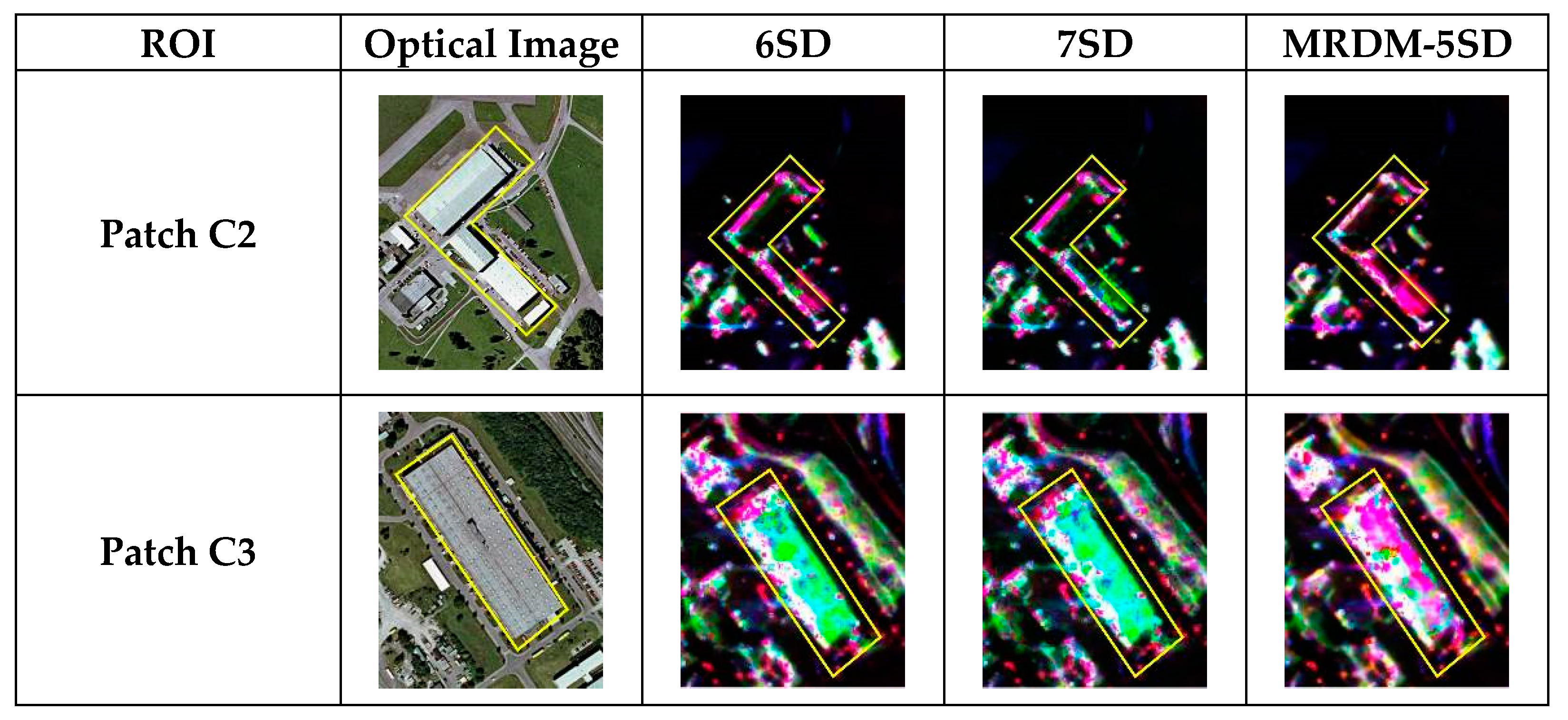
4.3. Validation by Airborne E-SAR Datasets

To further evaluate the adequacy of MRDM-5SD, airborne E-SAR L-Band data sets were used to analyze the decomposition performance. The observed scene is Oberpfaffenhofen, Germany, including areas of buildings, vegetation, airport and flatlands. The optical image is shown in Figure 14 and the decomposition results of Y4O, Y4R, G4U, 6SD, 7SD and MRDM-5SD are shown in Figure 15.

There is a large area of buildings to the right of the observed area, which exhibits intense red. The upper left is a lush vegetated area with strong volume scattering. Below are flat grounds such as airport runway, which should exhibit blue for surface scattering. However, the area is actually dark since the energy of surface scattering is weak.

In order to analyze the scattering of typical regions, five ROIs are selected. The detailed percentages of scattering contributions are listed in

Table 4. Scattering contributions (%) of Patch C1-C5 for E-SAR data sets.

ROIs	Methods	${\mathit{P}}_{\mathit{s}}$	${\mathit{P}}_{\mathit{d}}$	${\mathit{P}}_{\mathit{v}}$	${\mathit{P}}_{\mathit{h}}$	${\mathit{P}}_{\mathit{o}\mathit{d}}$	${\mathit{P}}_{\mathit{c}\mathit{d}}$	${\mathit{P}}_{\mathit{m}\mathit{d}}$
Patch C1	Y4O	33.0	54.2	11.1	1.7	-	-	-
	Y4R	33.2	54.6	10.6	1.6	-	-	-
	G4U	31.1	54.6	13.9	0.4	-	-	-
	6SD	32.9	56.9	5.8	1.5	1.6	1.3	-
	7SD	34.0	56.0	4.9	1.3	0.8	1.2	1.8
	MRDM-5SD	31.3	56.0	10.4	-	1.3	1.0	-
Patch C2	Y4O	24.1	21.9	48.4	5.6	-	-	-
	Y4R	27.2	28.0	39.4	5.4	-	-	-
	G4U	21.8	29.2	48.4	0.6	-	-	-
	6SD	20.8	38.4	17.7	2.1	8.9	12.1	-
	7SD	20.8	36.7	19.4	2.0	2.0	19.7	5.4
	MRDM-5SD	26.2	47.8	17.1	-	5.2	3.7	-
Patch C3	Y4O	57.6	5.8	31.1	5.5	-	-	-
	Y4R	65.4	12.3	18.6	3.7	-	-	-
	G4U	66.0	9.9	24.0	0.1	-	-	-
	6SD	50.2	23.8	20.5	1.5	2.5	1.5	-
	7SD	34.9	9.3	48.0	2.2	1.5	1.7	2.4
	MRDM-5SD	52.7	32.0	11.5	-	3.1	0.7	-
Patch C4	Y4O	80.7	7.6	5.9	5.8	-	-	-
	Y4R	80.5	7.8	5.9	5.8	-	-	-
	G4U	80.3	7.9	6.0	5.8	-	-	-
	6SD	71.7	7.3	5.3	5.2	5.3	5.2	-
	7SD	86.6	8.2	4.2	0.2	0.3	0.3	0.2
	MRDM-5SD	86.5	8.7	3.5	-	0.6	0.7	-
Patch C5	Y4O	21.0	26.8	49.7	2.5	-	-	-
	Y4R	21.2	26.9	49.3	2.6	-	-	-
	G4U	18.3	27.8	53.5	0.4	-	-	-
	6SD	24.8	30.0	36.8	2.6	3.1	2.7	-
	7SD	27.5	28.7	32.9	2.4	2.9	2.9	2.7
	MRDM-5SD	25.3	22.3	48.2	-	2.2	2.0	-

. Patch C1 is urban area perpendicular to the incident direction of radar, where double-bounce scattering is predominantly observed. The percentage of double-bounce scattering in MRDM-5SD is close to those of 6SD and 7SD. Patch C4 is a flat region with grassland, so surface scattering is dominant. The detailed surface scattering contributions of Y4O, Y4R, G4U, 6SD, 7SD and MRDM-5SD are 80.7%, 80.5%, 80.3%, 71.7%, 86.6% and 86.5%, respectively. Patch C5 is a vegetation area and volume scattering should be predominant. The percentage of volume scattering in MRDM-5SD is 48.2%, which is higher than the 36.8% of 6SD and 32.9% of 7SD.

Patch C2 and C3 are buildings with large orientation angles. The enlarged view is shown in Figure 16, in which only the decomposition results of 6SD, 7SD and MRDM-5SD are presented.

The double-bounce scattering contributions by Y4O, Y4R and G4U are weak, so the results are not satisfactory. Patch C2 is an L-shaped building area with large orientation angles. Both 6SD and 7SD can extract strong double-bounce scattering contributions, making the whole region exhibit red. However, MRDM-5SD can significantly increase the double-bounce scattering component. The percentage of double-bounce scattering in this area from MRDM-5SD is 47.8%, which is even higher than those of 6SD and 7SD. Moreover, the volume scattering component is reduced with use of MRDM-5SD as well. Patch C3 is another building with large orientation angle. The contribution of double-bounce scattering from 6SD reaches 23.8% and that of volume scattering reaches 20.5%. However, due to the large roof of the building, strong surface scattering is also generated, so the whole area exhibits blue-green. The double-bounce scattering contribution from 7SD is weak. MRDM-5SD improves the double-bounce scattering percentage to 32.0% and reduces the percentage of volume scattering to 11.5%, making the area exhibit red.

As can be seen from the above experimental results, MRDM-5SD can achieve better decomposition results compared with other existing decomposition methods. Especially in urban areas with large orientation angles, the contribution of double-bounce scattering can be greatly improved.

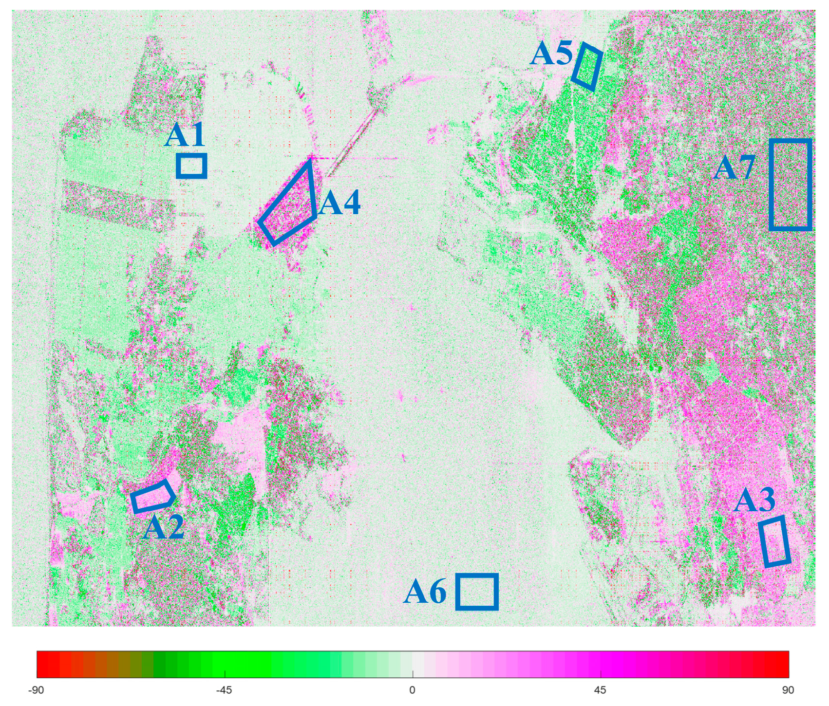
4.4. Building Detection for ALOS-2/PALSAR-2 Datasets

The superiority of MRDM-5SD is further confirmed at the application level. Since MRDM-5SD modifies the double-bounce scattering model, the reliability of the decomposition method is verified via building detection experiments.

The ALOS-2/PALSAR-2 datasets were used for detection and an area of $2000\times 2700$ pixels was selected. The ground objects in this scene include water, vegetation and urban buildings. The traditional support vector machine (SVM) was used for building detection and the scattering contributions extracted using each polarimetric decomposition method are input. We chose 400 pixels each from water areas, vegetation areas and urban building areas as training samples. The ground truth is shown in Figure 17a, which is based on the Y4R decomposition result. Building areas are marked in red. The detection results of Y4R, G4U, 6SD, 7SD and MRDD-5SD decomposition are shown in Figure 17b–f, respectively.

It can be seen from the figure that MRDD-5SD has better effects of building detection, especially in urban areas with large orientation angles. More buildings are detected in Figure 17f and the miss rate is reduced. In order to compare the detection results in detail, the precision rate, false alarm rate and miss rate were calculated and are shown in

Table 5. Comparison of detection results from different decomposition methods.

Decomposition Methods	Precision Rate (%)	False Alarm Rate (%)	Miss Rate (%)
Y4R	87.50	4.83	6.00
G4U	85.03	6.00	5.35
6SD	85.14	5.96	5.14
7SD	85.54	5.63	7.40
MRDD-5SD	92.33	2.87	3.88

.

According to the evaluation index, the best detection result is observed when MRDD-5SD decomposition is used. The precision rate is 92.33%, which is higher than any other methods. The false alarm rate and miss rate are also reduced compared with detection experiments using other decomposition methods. It can be concluded that MRDD-5SD performs better in urban areas. In areas of buildings with large orientation angles, MRDD-5SD can effectively increase the proportion of double-bounce scattering and thus reduce the miss rate of buildings in such areas.

5. Conclusions

In this paper, a modified rotational dihedral model (MRDM) is proposed. Based on electromagnetic analysis and calculation, the scattering of a rotational dihedral was analyzed using high-frequency approximation methods. In this case, MRDM is proposed to describe the scattering mechanism of rotational dihedrals accurately. MRDM was further introduced to a five-component decomposition method (MRDM-5SD). The decomposition method was validated using spaceborne L-band ALOS-2/PALSAR-2, spaceborne C-band GF-3, and airborne L-band E-SAR datasets. The experiments show that MRDM-5SD can effectively improve the double-bounce scattering contribution in urban areas, especially those with large orientation angles. The percentage of double-bounce scattering in highly oriented urban area can be greatly improved compared with advanced existing decomposition methods. The superiority of the proposed method was further verified via building detection experiments. Therefore, MRDM-5SD based on MRDM can extract effective features of urban areas and other regions, which can provide support for the application of PolSAR data.

References

1. Lee, J.S.; Pottier, E. Overview of polarimetric radar imaging. In Polarimetric Radar Imaging from Basics to Applications; Taylor & Francis Group: Boca Raton, FL, USA, 2009; pp. 5–13. [Google Scholar]
2. Cloude, S.R. Depolarisation and scattering entropy. In Polarization Applications in Remote Sensing; Oxford University Press: Oxford, UK, 2010; pp. 71–118. [Google Scholar]
3. Aghababaee, H.; Sahebi, M.R. Model-based target scattering decomposition of polarimetric SAR tomography. IEEE Trans. Geosci. Remote Sens. 2018, 56, 972–983. [Google Scholar] [CrossRef]
4. Pallotta, L.; Orlando, D. Polarimetric covariance eigenvalues classification in SAR images. IEEE Geosci. Remote Sens. Lett. 2019, 16, 746–750. [Google Scholar] [CrossRef]
5. Li, Y.; Yin, Q.; Lin, Y.; Hong, W. Anisotropy scattering detection from multiaspect signatures of circular polarimetric SAR. IEEE Trans. Geosci. Remote Sens. 2018, 15, 1575–1579. [Google Scholar] [CrossRef]
6. Liu, C.; Yang, J.; Ou, J.; Fan, D. Offshore bridge detection in Polarimetric SAR images based on water network construction using Markov tree. Remote Sens. 2022, 14, 3888. [Google Scholar] [CrossRef]
7. Zhang, T.; Wang, W.; Yang, Z.; Yin, J.; Yang, J. Ship detection from PolSAR imagery using the hybrid polarimetric covariance matrix. IEEE Geosci. Remote Sens. Lett. 2021, 18, 1575–1579. [Google Scholar] [CrossRef]
8. Li, H.; Cui, X.; Chen, S.; Yang, J. PolSAR ship detection with optimal polarimetric rotation domain features and SVM. Remote Sens. 2021, 13, 3932. [Google Scholar] [CrossRef]
9. Richards, J.A. Interpretation based on structural models. In Remote Sensing with Imaging Radar; Springer: Berlin/Heidelberg, Germany, 2009; pp. 281–301. [Google Scholar]
10. Cui, Y.; Yamaguchi, Y.; Yang, J.; Kobayashi, H.; Park, S.; Singh, G. On complete model-based decomposition of polarimetric SAR coherency matrix data. IEEE Trans. Geosci. Remote Sens. 2014, 52, 1991–2001. [Google Scholar] [CrossRef]
11. An, W.; Lin, M. An incoherent decomposition algorithm based on polarimetric symmetry for multilook polarimetric SAR data. IEEE Trans. Geosci. Remote Sens. 2020, 58, 2383–2397. [Google Scholar] [CrossRef]
12. Mohanty, S.; Singh, G. Improved POLSAR model-based decomposition interpretation under scintillation conditions. IEEE Trans. Geosci. Remote Sens. 2019, 57, 7567–7578. [Google Scholar] [CrossRef]
13. Ainsworth, T.L.; Wang, Y.; Lee, J.S. Model-based polarimetric SAR decomposition: An L1 regularization approach. IEEE Trans. Geosci. Remote Sens. 2022, 60, 5208013. [Google Scholar] [CrossRef]
14. Freeman, A.; Durden, S.L. A three-component scattering model for polarimetric SAR data. IEEE Trans. Geosci. Remote Sens. 1998, 36, 963–973. [Google Scholar] [CrossRef] [Green Version]
15. Singh, G.; Yamaguchi, Y.; Park, S. General four-component scattering power decomposition with unitary transformation of coherency matrix. IEEE Trans. Geosci. Remote Sens. 2013, 51, 3014–3022. [Google Scholar] [CrossRef]
16. Chen, S.; Wang, X.; Xiao, S.; Sato, M. General polarimetric model-based decomposition for coherency matrix. IEEE Trans. Geosci. Remote Sens. 2014, 52, 1843–1855. [Google Scholar] [CrossRef]
17. Yamaguchi, Y.; Moriyama, T.; Ishido, M.; Yamada, H. Four-component scattering model for polarimetric SAR image decomposition. IEEE Trans. Geosci. Remote Sens. 2005, 43, 1699–1706. [Google Scholar] [CrossRef]
18. Sato, A.; Yamaguchi, Y.; Singh, G.; Park, S. Four-component scattering power decomposition with extended volume scattering model. IEEE Geosci. Remote Sens. Lett. 2012, 9, 160–171. [Google Scholar] [CrossRef]
19. Yamaguchi, Y.; Sato, A.; Boerner, W.; Sato, R.; Yamada, H. Four-component scattering power decomposition with rotation of coherency matrix. IEEE Trans. Geosci. Remote Sens. 2011, 49, 2251–2258. [Google Scholar] [CrossRef]
20. Singh, G.; Yamaguchi, Y. Model-based six-component scattering matrix power decomposition. IEEE Trans. Geosci. Remote Sens. 2018, 56, 5687–5704. [Google Scholar] [CrossRef]
21. Singh, G.; Malik, R.; Mohanty, S.; Rathore, V.S.; Yamada, K.; Umemura, M.; Yamaguchi, Y. Seven-component scattering power decomposition of POLSAR coherency matrix. IEEE Trans. Geosci. Remote Sens. 2019, 57, 8371–8382. [Google Scholar] [CrossRef]
22. Maurya, H.; Panigrahi, R.K. PolSAR coherency matrix optimization through selective unitary rotations for model-based decomposition scheme. IEEE Geosci. Remote Sens. Lett. 2019, 16, 658–662. [Google Scholar] [CrossRef]
23. Wang, Y.; Yu, W.; Liu, X.; Wang, C.; Kuijper, A.; Guthe, S. Demonstration and analysis of an extended adaptive general four-component decomposition. IEEE J. Sel. Top. Appl. Earth. Obs. Remote Sens. 2020, 13, 2573–2586. [Google Scholar] [CrossRef]
24. Yin, Q.; Xu, J.; Xiang, D.; Zhou, Y.; Zhang, F. Polarimetric decomposition with an urban area descriptor for compact polarimetric SAR data. IEEE J. Sel. Top. Appl. Earth. Obs. Remote Sens. 2021, 14, 10033–10044. [Google Scholar] [CrossRef]
25. Zhang, L.; Chen, Y.; Wang, N.; Zou, B.; Liu, S. Scattering mechanism analysis of man-made targets via polarimetric SAR observation simulation. IEEE J. Sel. Top. Appl. Earth. Obs. Remote Sens. 2022, 15, 919–929. [Google Scholar] [CrossRef]
26. Gordon, W. Far-field approximations to the Kirchoff-Helmholtz representations of scattered fields. IEEE Trans. Antennas Propag. 1975, 23, 590–592. [Google Scholar] [CrossRef]
27. Giorgio, F.; Riccio, D. Analytic formulations of electromagnetic scattering. In Scattering, Natural Surfaces, and Fractals; Elsevier: Burlington, MA, USA, 2006; p. 130. [Google Scholar]
28. Chai, S.R.; Guo, L.X.; Li, K.; Li, L. Combining CS with FEKO for fast target characteristic acquisition. IEEE Trans. Antennas Propag. 2018, 66, 2494–2504. [Google Scholar] [CrossRef]
29. Lee, J.S.; Schuler, D.L.; Ainsworth, T.L. Polarimetric SAR data compensation for terrain azimuth slope variation. IEEE Trans. Geosci. Remote Sens. 2000, 38, 2153–2163. [Google Scholar]
30. Chen, Q.; Jiang, Y.M.; Zhao, L.J.; Kuang, G.Y. Polarimetric scattering similarity between a random scatterer and a canonical scatterer. IEEE Geosci. Remote Sens. Lett. 2010, 7, 866–869. [Google Scholar] [CrossRef]
31. Maurya, H.; Panigrahi, R.K. Investigation of branching conditions in model-based decomposition methods. IEEE Geosci. Remote Sens. Lett. 2018, 15, 1224–1228. [Google Scholar] [CrossRef]
Figure 1. Dihedral scattering analysis model.
Remotesensing 15 00101 g001
Figure 2. Comparison of parametric scattering model with different relative permittivities.
Remotesensing 15 00101 g002
Figure 3. Comparison of parametric scattering model with different conductivities.
Remotesensing 15 00101 g003
Figure 4. Comparison of parametric scattering model with different look angles.
Remotesensing 15 00101 g004
Figure 5. Comparison of parametric scattering model with different orientation angles.
Remotesensing 15 00101 g005
Figure 6. Flowchart of MRDM-5SD.
Remotesensing 15 00101 g006
Figure 7. Optical image of the observed area from Google Earth.
Remotesensing 15 00101 g007
Figure 8. Orientation angle estimation of ALOS-2/PALSAR-2 data sets.
Remotesensing 15 00101 g008
Figure 9. Decomposition results of ALOS-2/PALSAR-2 data sets over San Francisco (RGB component: red: double-bounce scattering, green: volume scattering, blue: surface scattering). (a) Y4O, (b) Y4R, (c) G4U, (d) 6SD, (e) 7SD, (f) MRDM-5SD.
Remotesensing 15 00101 g009
Figure 10. Enlarged view of Patch A1 (orthogonal urban area), Patch A2, A3 (urban areas with moderate orientation angles), Patch A4, A5 (urban areas with large orientation angles), Patch A6 (water body), Patch A7 (hilly terrain) by Y4R, 7SD and MRDM-5SD (RGB component: red: double-bounce scattering, green: volume scattering, blue: surface scattering).
Remotesensing 15 00101 g010
Figure 11. Optical image of GF-3 data sets from Google Earth.
Remotesensing 15 00101 g011
Figure 12. Decomposition results of GF-3 data sets over Harbin, China (RGB component: red: double-bounce scattering, green: volume scattering, blue: surface scattering). (a) Y4O, (b) Y4R, (c) G4U, (d) 6SD, (e) 7SD, (f) MRDM-5SD.
Remotesensing 15 00101 g012aRemotesensing 15 00101 g012b
Figure 13. Enlarged view of Patch B3 (a) optical image, (b) Y4O, (c) Y4R, (d) G4U, (e) 6SD, (f) 7SD, (g) MRDM-5SD (RGB component: red: double-bounce scattering, green: volume scattering, blue: surface scattering).
Remotesensing 15 00101 g013
Figure 14. Optical image of Oberpfaffenhofen, Germany.
Remotesensing 15 00101 g014
Figure 15. Decomposition results of E-SAR data sets over Oberpfaffenhofen, Germany (RGB component: red: double-bounce scattering, green: volume scattering, blue: surface scattering). (a) Y4O, (b) Y4R, (c) G4U, (d) 6SD, (e) 7SD, (f) MRDM-5SD.
Remotesensing 15 00101 g015
Figure 16. Enlarged view of Patch C2 and C3 (both highly oriented buildings) via 6SD, 7SD and MRDM-5SD (RGB component: red: double-bounce scattering, green: volume scattering, blue: surface scattering).
Remotesensing 15 00101 g016
Figure 17. Building detection results of ALOS-2/PALSAR-2 dataset. (a) Ground truth image, (b) Y4R, (c) G4U, (d) 6SD, (e) 7SD, (f) MRDD-5SD.
Remotesensing 15 00101 g017aRemotesensing 15 00101 g017b