
Quick Quality Assessment and Radiometric Calibration of C-SAR/01 Satellite Using Flexible Automatic Corner Reflector

 ,
,
Abstract
:
1. Introduction
2. Study Area and Data
2.1. Experimental Area
2.2. Remote Sensing Data
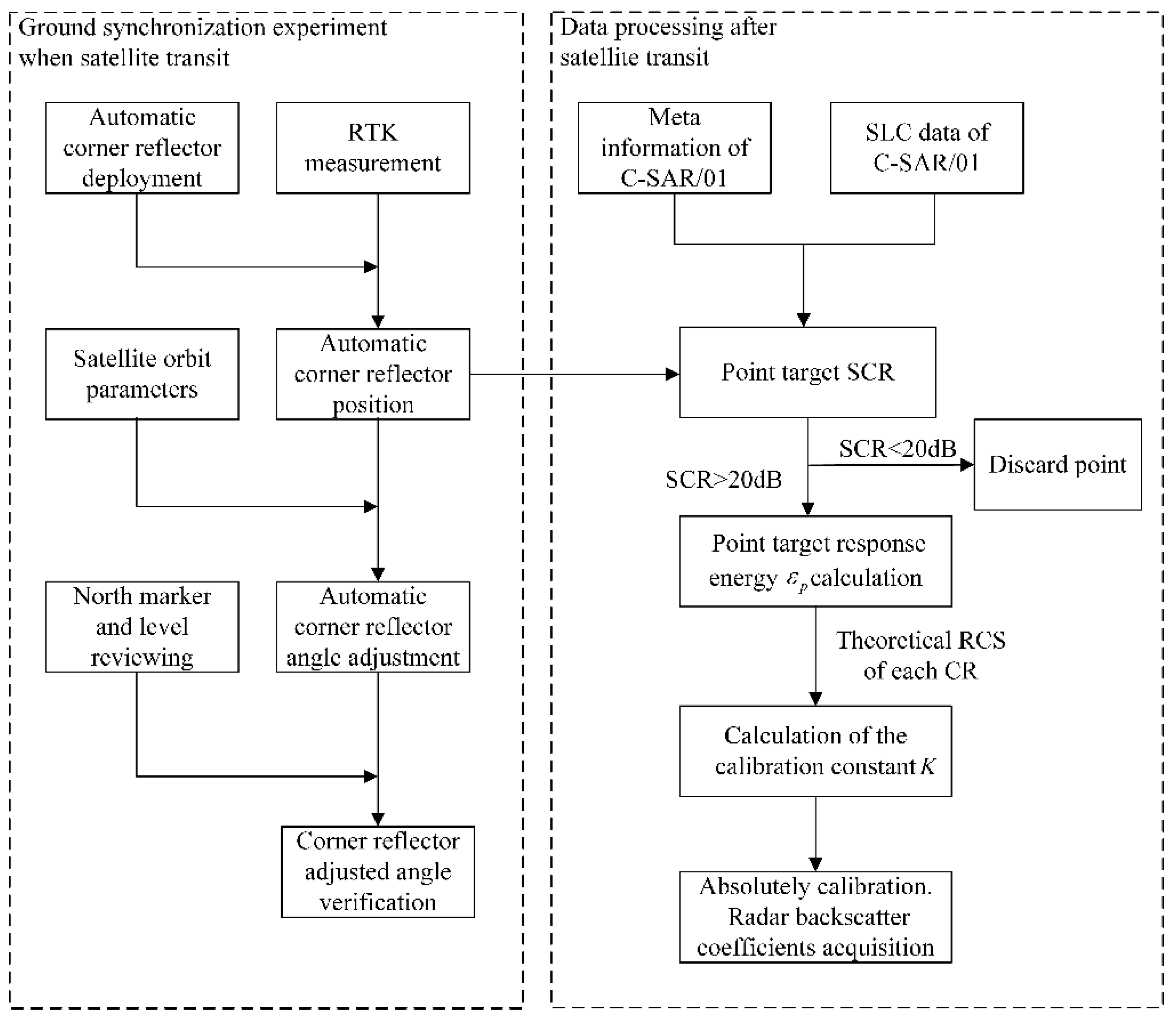
2.3. Ground Synchronous Measurement
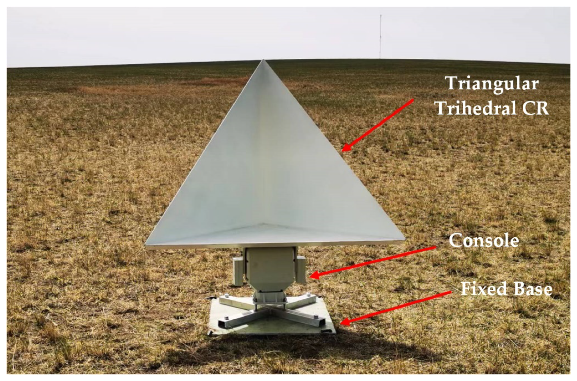
2.3.1. Flexible Automatic Trihedral Corner Reflector
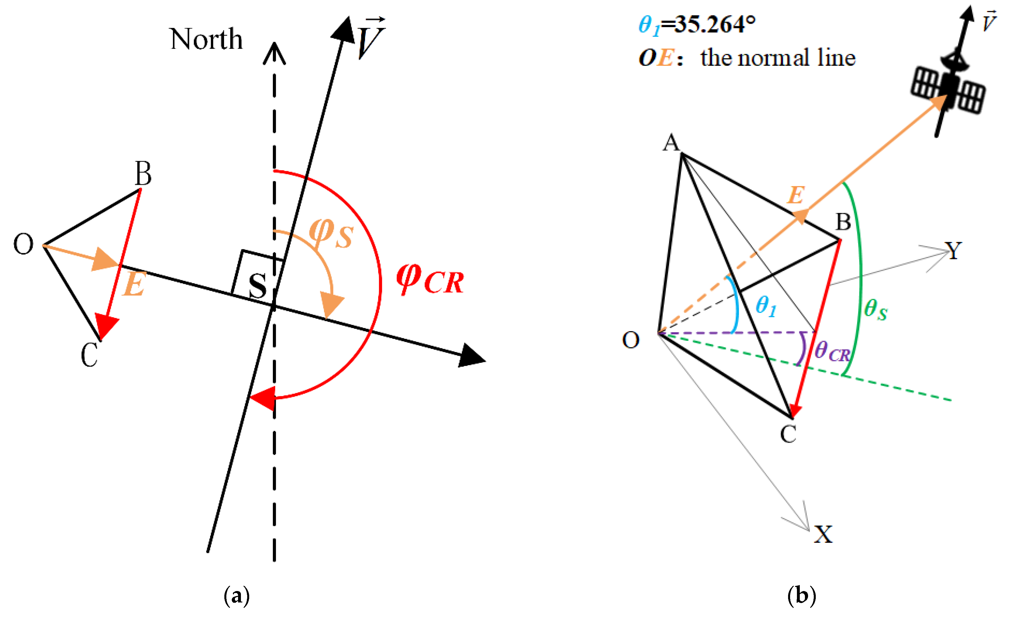
2.3.2. Azimuth and Elevation Angle of CR Calculation
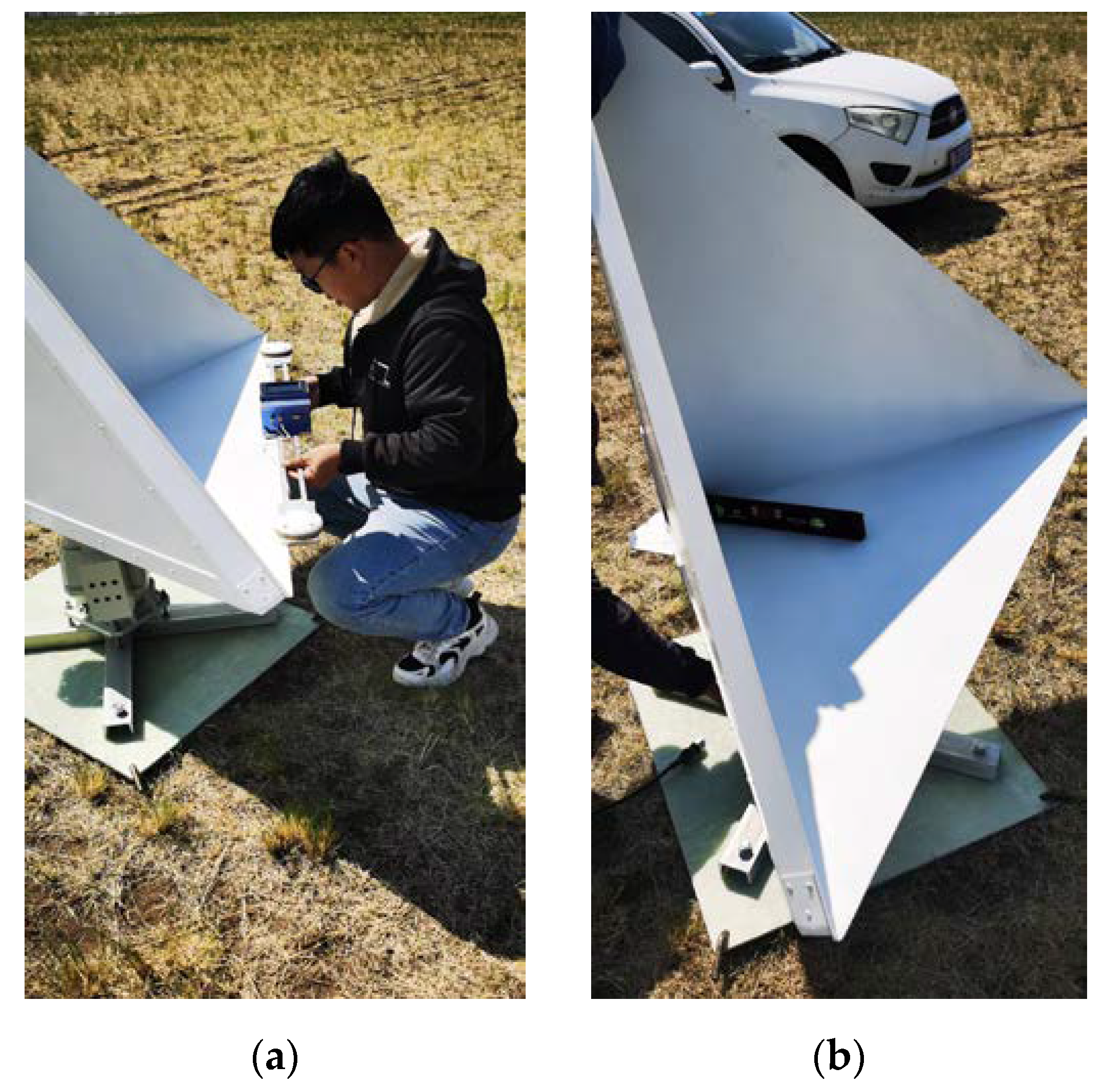
2.3.3. Auxiliary Parameter Measurement
3. Method
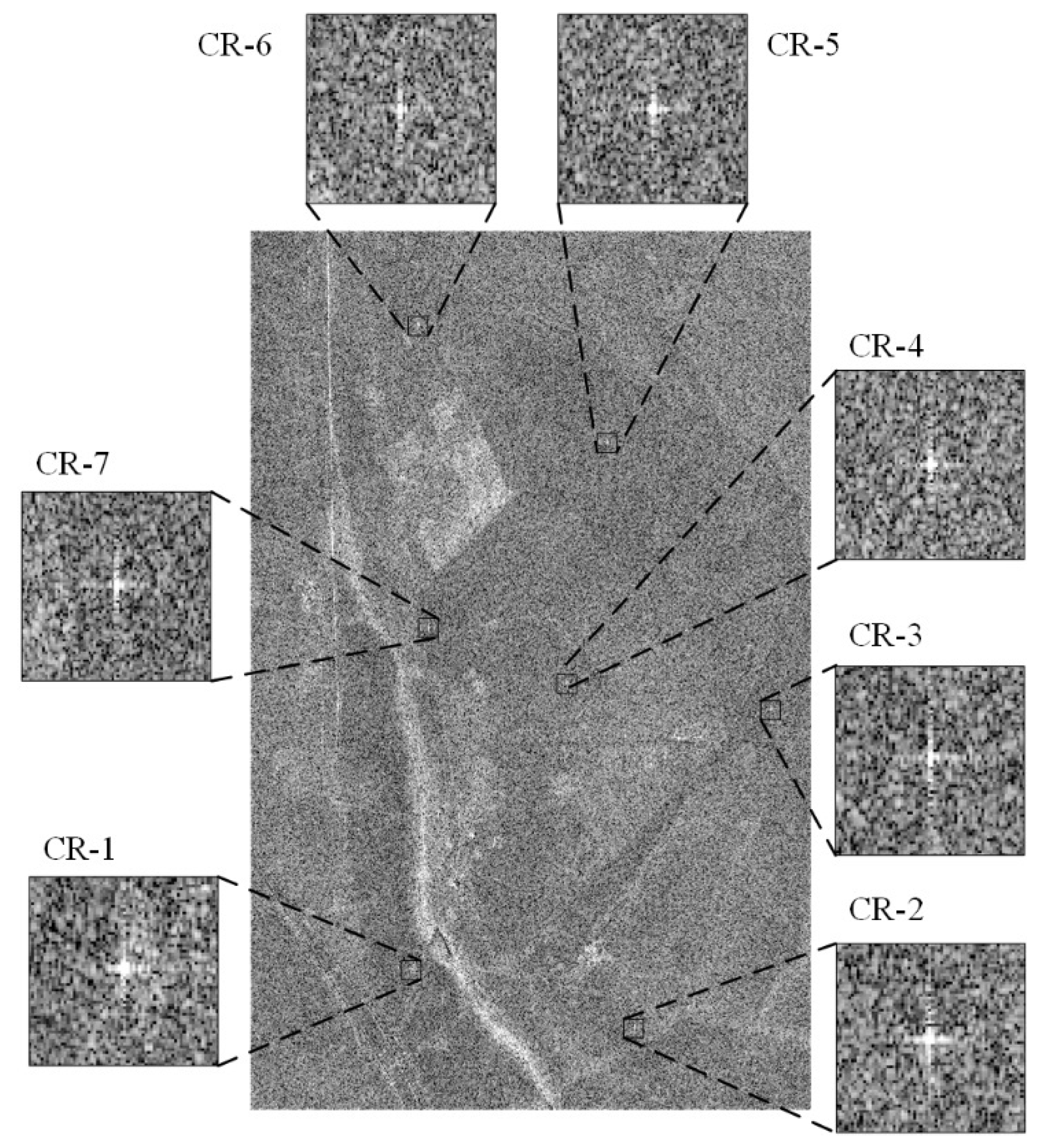
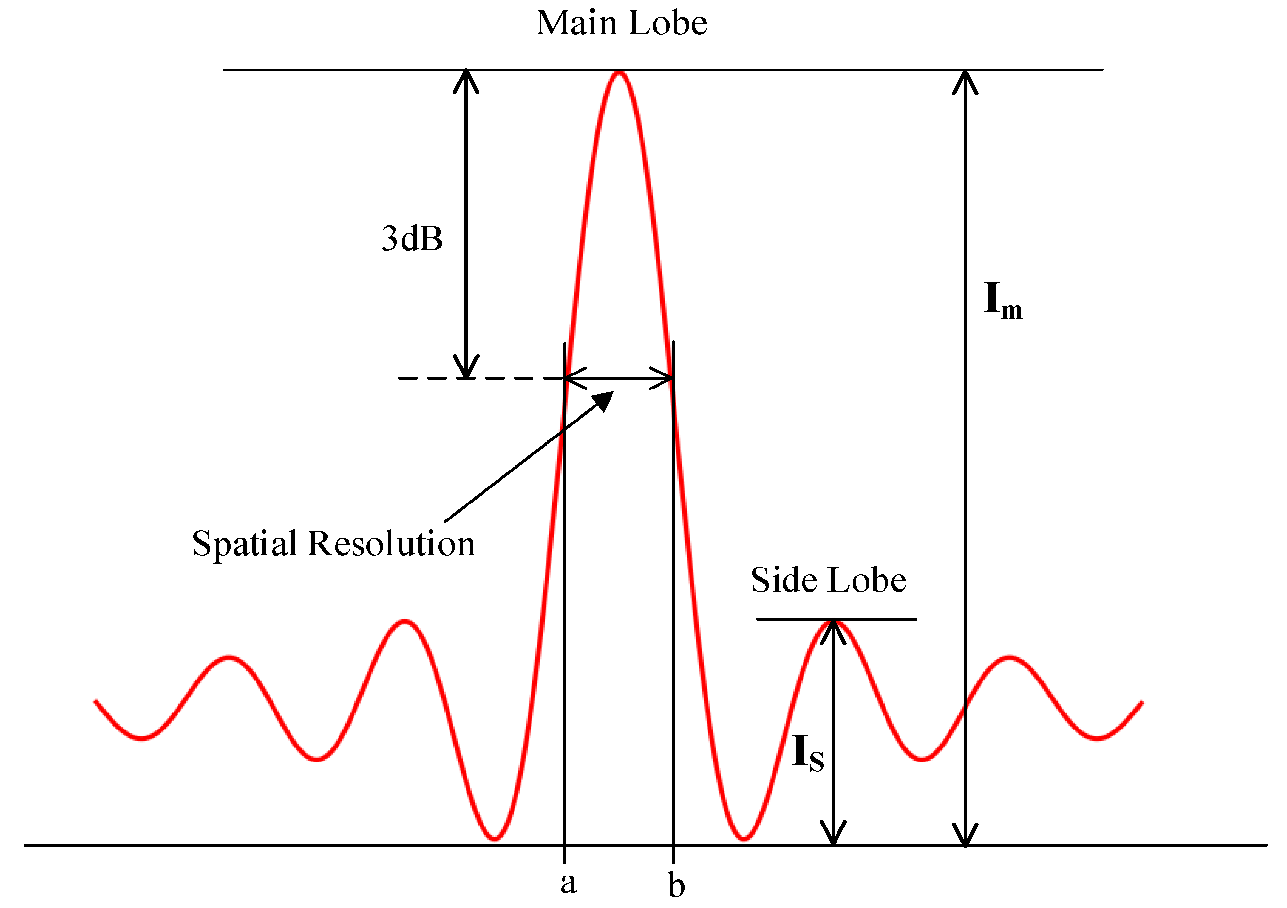
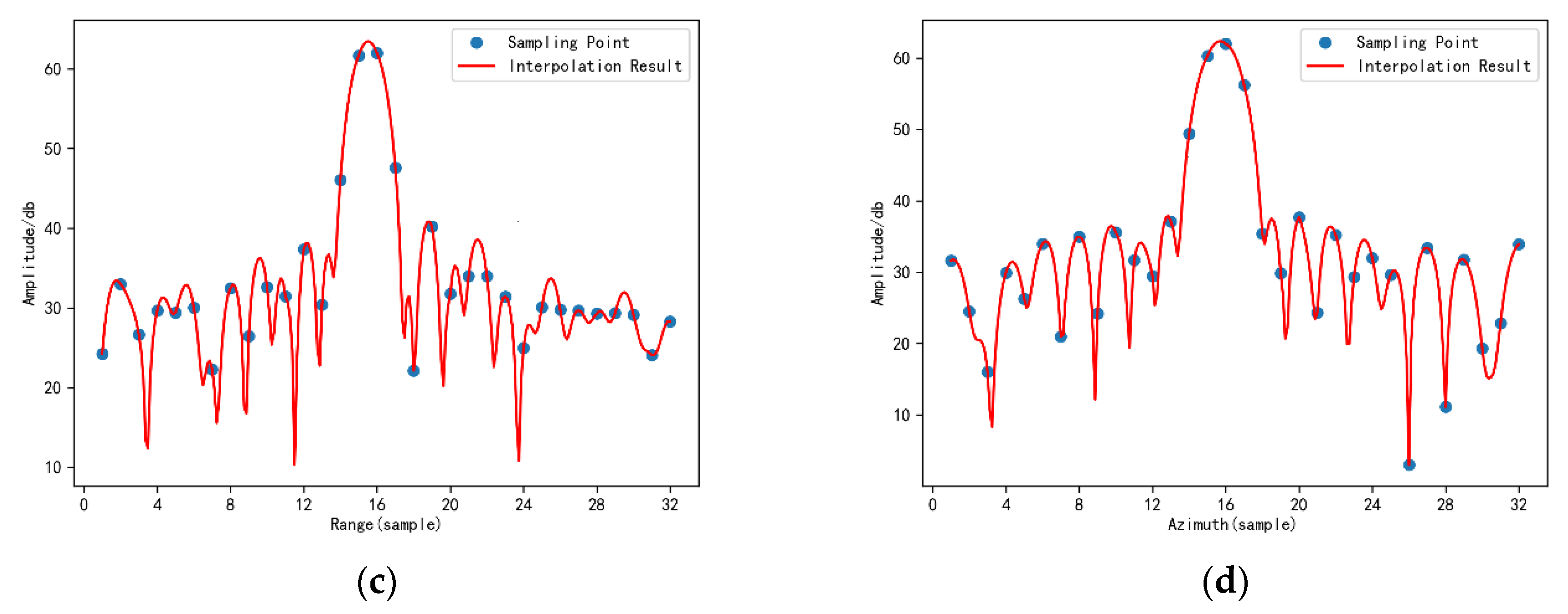
3.1. SCR Analysis
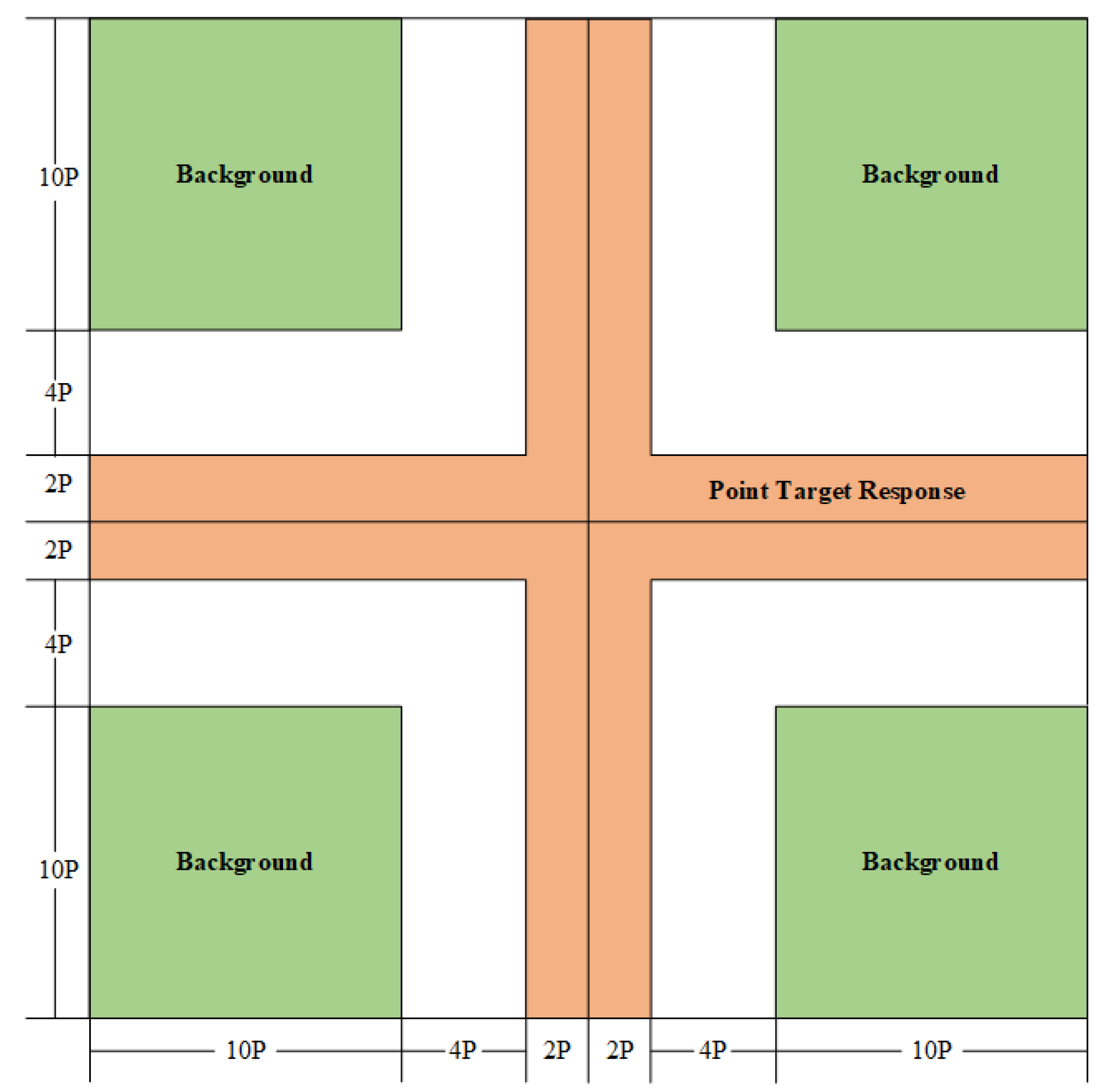
3.2. Point Target Response Energy Calculation
3.3. Calculation of the Calibration Constant
4. Image Quality Assessment Results
5. Radiometric Calibration Processing Results
5.1. Point Target SCR Analysis
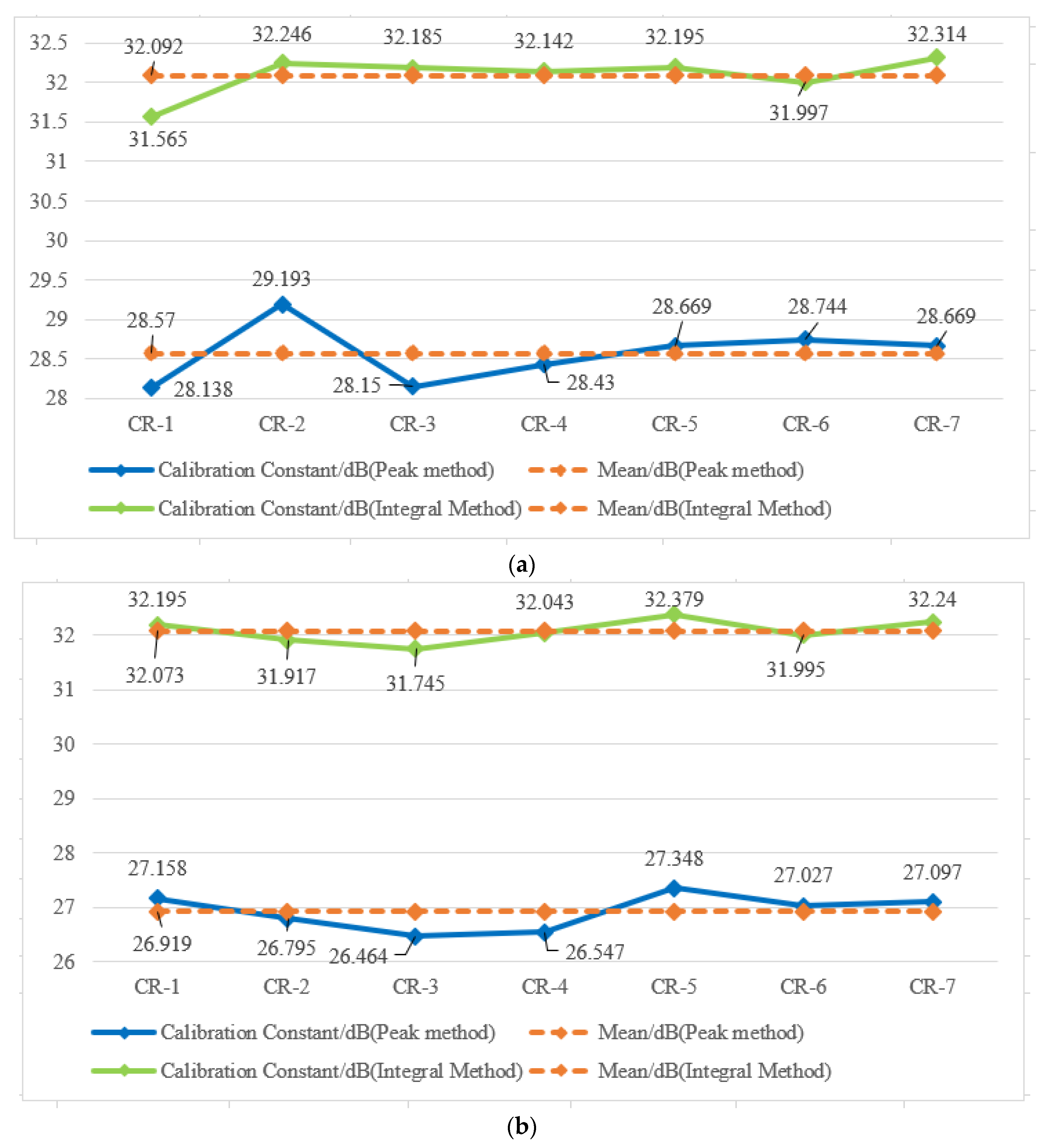
5.2. Response Energy and Calibration Constant Calculation
5.3. Backscattering Coefficient Calculation and Calibration Accuracy Analysis
6. Discussion
7. Conclusions
Author Contributions
Funding
Data Availability Statement
Conflicts of Interest
References
- Moreira, A. A golden age for spaceborne SAR systems. In Proceedings of the 2014 20th International Conference on Microwaves, Radar and Wireless Communications (MIKON), Gdansk, Poland, 16–18 June 2014; pp. 1–4. [Google Scholar]
- Freeman, A. SAR calibration: An overview. IEEE Trans. Geosci. Remote Sens. 1992, 30, 1107–1121. [Google Scholar] [CrossRef]
- Schwerdt, M.; Brautigam, B.; Bachmann, M.; Doring, B.; Schrank, D.; Gonzalez, J.H. Final TerraSAR-X Calibration Results Based on Novel Efficient Methods. IEEE Trans. Geosci. Remote Sens. 2010, 48, 677–689. [Google Scholar] [CrossRef]
- Schmidt, K.; Ramon, N.T.; Schwerdt, M. Radiometric Accuracy and Stability of Sentinel-1A Determined using Point Targets. Int. J. Microw. Wirel. Technol. 2018, 10, 538–546. [Google Scholar] [CrossRef] [Green Version]
- Schwerdt, M.; Schmidt, K.; Ramon, N.T.; Klenk, P.; Yague-Martinez, N.; Prats-Iraola, P.; Zink, M.; Geudtner, D.; Chapman, B.; Siqueira, P.; et al. Independent System Calibration of Sentinel-1B. Remote Sens. 2017, 9, 511. [Google Scholar] [CrossRef] [Green Version]
- Mishra, M.; Pate, P.; Srivastava, H.S.; Patel, P.R.; Shukla, A.K. Absolute Radiometric Calibration of FRS -1 and MRS mode of RISAT-1 Synthetic Aperture Radar (SAR) data using Corner Reflectors. Int. J. Adv. Eng. Res. Sci. (IJAERS) 2014, 1, 78–89. [Google Scholar]
- Srivastava, S.; Cote, S.; Muir, S. The RADARSAT-1 imaging performance, 14 years after launch, and independent report on RADARSAT-2 image quality. In Proceedings of the 2010 IEEE International Geoscience and Remote Sensing Symposium, Honolulu, HI, USA, 25–30 July 2010; pp. 3458–3461. [Google Scholar]
- Gisinger, C.; Schubert, A.; Breit, H.; Garthwaite, M.; Balss, U.; Willberg, M.; Small, D.; Eineder, M.; Miranda, N. In-Depth Verification of Sentinel-1 and TerraSAR-X Geolocation Accuracy Using the Australian Corner Reflector Array. IEEE Trans. Geosci. Remote Sens. 2021, 59, 1154–1181. [Google Scholar] [CrossRef]
- Zhou, X.; Zeng, Q.; Jiao, J.; Wang, Q.; Xiong, S.; Gao, S. Field calibration and validation of Radarsat-2. In Proceedings of the 2013 IEEE International Geoscience and Remote Sensing Symposium (IGARSS), Melbourne, Australia, 21–26 July 2013; pp. 4451–4454. [Google Scholar]
- Praveen, T.N.; Raju, M.V.; Vishwanath, B.D.; Meghana, P.; Manjula, T.R.; Raju, G. Absolute radiometric calibration of RISAT-1 SAR image using peak method. In Proceedings of the 2018 3rd IEEE International Conference on Recent Trends in Electronics, Information & Communication Technology (RTEICT), Bengaluru, India, 18–19 May 2018; pp. 456–460. [Google Scholar]
- Dring, B.; Schwerdt, M.; Bauer, R. TerraSAR-X Calibration Ground Equipment. In Proceedings of the Wave Propagation in Communication, Microwaves Systems and Navigation -2007 (WFMN07), Chemnitz, Germany, 4–5 July 2007; pp. 86–90. [Google Scholar]
- Sharma, S.; Dadhich, G.; Rambhia, M.; Mathur, A.K.; Prajapati, R.P.; Patel, P.R.; Shukla, A. Radiometric calibration stability assessment for the RISAT-1 SAR sensor using a deployed point target array at the Desalpar site, Rann of Kutch, India. Int. J. Remote Sens. 2017, 38, 7242–7259. [Google Scholar] [CrossRef]
- Chang, Y.; Li, P.; Yang, J.; Zhao, J.; Zhao, L.; Shi, L. Polarimetric Calibration and Quality Assessment of the GF-3 Satellite Images. Sensors 2018, 18, 403–415. [Google Scholar] [CrossRef] [PubMed] [Green Version]
- Doerry, A.W. Reflectors for SAR Performance Testing; Technical Report; Sandia National Laboratories: Albuquerque, NM, USA; Livermore, CA, USA, 2008. [Google Scholar]
- Ye, X.; Kaufmann, H.; Guo, X. Differential SAR Interferometry Using Corner Refletors. In Proceedings of the 2002 IEEE International Geoscience & Remote Sensing Symposium, Toronto, Canada, 24–28 June 2002; pp. 1243–1246. [Google Scholar]
- Liu, Y. Research on Low Earth Orbit Spacecraft Orbit Prediction Strategy Based on SGP4 Model. Master’s Dissertation, Harbin Institute of Technology, Harbin, China, 2009. [Google Scholar]
- Yang, S.; Xu, Z.; Cheng, C. Method of airborne SAR radiation calibration based on point target. In Proceedings of the International Archives of the Photogrammetry, Remote Sensing and Spatial Information Sciences—ISPRS Archives, Online, 14–20 June 2020; pp. 123–128. [Google Scholar]
- Zongmin, F.; Lei, H.; Zhihua, T.; Jiuli, L.; Liangbo, Z. Airborne SAR radiometric calibration using point targets. IOP Conf. Ser. Earth Environ. Sci. 2014, 17, 012186. [Google Scholar] [CrossRef] [Green Version]
- Touzi, R.; Hawkins, R.K.; Cote, S. High-Precision Assessment and Calibration of Polarimetric RADARSAT-2 SAR Using Transponder Measurements. IEEE Trans. Geosci. Remote Sens. 2013, 51, 487–503. [Google Scholar] [CrossRef]
- Ulander, I.M.H. Accuracy of using point targets for SAR calibration. IEEE Trans. Aerosp. Electron. Syst. 1991, 27, 139–148. [Google Scholar] [CrossRef]
- Gray, A.L.; Vachon, P.W. Synthetic aperture radar calibration using reference reflectors. IEEE Trans. Geosci. Remote Sens. 1990, 28, 374–383. [Google Scholar] [CrossRef]
- Yuan, L.; Li, Z.; Ge, J.; Jiang, K. Research on Approach of SAR Radiometric Calibration Using Point Target. Radio Eng. 2009, 39, 25–28. [Google Scholar]
- Li, L.; Zhang, F.; Shao, Y.; Wei, Q.; Huang, Q.; Jiao, Y. Airborne SAR Radiometric Calibration Based on Improved Sliding Window Integral Method. Sensors 2022, 22, 320. [Google Scholar] [CrossRef] [PubMed]
- Zhao, L.; Li, Y.; Zhang, Q.; Liu, J.; Yuan, X.; Chen, Q. Design and Verification of Image Quality Indexes of GF-3 Satellite. Spacecr. Eng. 2017, 26, 18–23. [Google Scholar]
- Martinez, A.; Marchand, J.L. Implementation and quality analysis of a CSA SAR processor. In Proceedings of the IGARSS ’93-IEEE International Geoscience and Remote Sensing Symposium, Tokyo, Japan, 18–21 August 1993; pp. 1179–1181. [Google Scholar]
- Vu, V.T.; Sjögren, T.K.; Pettersson, M.I.; Gustavsson, A. Definition on SAR image quality measurements for UWB SAR. In Proceedings of the Proc. SPIE Image and Signal Process. Remote Sens. XIV, Cardiff, UK, 15 September 2008; pp. 71091A.71091–71091A.71099. [Google Scholar]
- Kuang, G.; Gao, G.; Jiang, Y. Synthetic Aperture Radar Target Detection Theory Algorithms and Applications; National University of Defense Technology Press: Changsha, China, 2007. [Google Scholar]
- Cumming, I.G.; Wong, F.H. Digital Signal Processing of Synthetic Aperture Radar Data: Algorithms and Implementation; Artech House: Boston, MA, USA; London, UK, 2005. [Google Scholar]


| Imaging Mode | Nominal Resolution /m | Imaging Swath /km | Polarization Mode | |
|---|---|---|---|---|
| Spotlight (SL) | 1 | 10 | Single | |
| Strip | Ultra-Fine Strip (UFS) | 3 | 30 | Single |
| Fine Strip I (FSI) | 5 | 50 | Dual | |
| Fine Strip II (FSII) | 10 | 100 | Dual | |
| Standard Strip (SS) | 25 | 130 | Dual | |
| Quad Polarization Strip I (QPSI) | 8 | 30 | Full (Quad) | |
| Quad Polarization Strip II (QPSII) | 25 | 40 | Full (Quad) | |
| Scan | Narrow ScanSAR (NSC) | 50 | 300 | Dual |
| Wide ScanSAR (WSC) | 100 | 500 | Dual | |
| Global Observation (GLO) | 500 | 650 | Dual | |
| Wave (WAV) | 8 | 20 | Full (Quad) | |
| Expanded incidence angle (EXT) | Low Incidence | 25 | 130 | Dual |
| High Incidence | 25 | 80 | Dual | |
| Date | Orbit Direction | Look Direction | Imaging Mode | Incidence Angle/° | Polarization | Nominal Resolution/m | Azimuth Pixel Size/m | Range Pixel Size/m |
|---|---|---|---|---|---|---|---|---|
| 12 May 2022 | Descending | Right | UFS | 28.43~30.57 | HH | 3 | 1.669818 | 1.124222 |
| 15 May 2022 | Ascending | Right | FSI | 26.01~29.60 | HH/HV | 5 | 2.613357 | 1.124222 |
| CR Number | Resolution (m) | PSLR (dB) | ISLR (dB) | |||
|---|---|---|---|---|---|---|
| Range | Azimuth | Range | Azimuth | Range | Azimuth | |
| CR-1 | 1.353 | 2.887 | −22.195 | −23.274 | −21.802 | −21.268 |
| CR-2 | 1.388 | 2.862 | −24.944 | −23.353 | −22.745 | −19.93 |
| CR-3 | 1.353 | 2.887 | −22.087 | −23.885 | −21.554 | −20.633 |
| CR-4 | 1.370 | 2.887 | −22.955 | −24.332 | −21.922 | −21.083 |
| CR-5 | 1.370 | 2.887 | −22.204 | −25.205 | −21.259 | −21.116 |
| CR-6 | 1.353 | 2.862 | −22.45 | −23.386 | −21.845 | −18.792 |
| CR-7 | 1.370 | 2.862 | −22.988 | −23.735 | −21.842 | −21.29 |
| Mean | 1.365 | 2.876 | −22.832 | −23.881 | −21.853 | −20.587 |
| CR Number | Resolution (m) | PSLR (dB) | ISLR (dB) | |||
|---|---|---|---|---|---|---|
| Range | Azimuth | Range | Azimuth | Range | Azimuth | |
| CR-1 | 1.651 | 4.881 | −23.047 | −24.345 | −21.831 | −19.536 |
| CR-2 | 1.616 | 4.760 | −23.361 | −24.533 | −17.211 | −20.467 |
| CR-3 | 1.616 | 4.760 | −22.63 | −24.473 | −21.464 | −18.514 |
| CR-4 | 1.599 | 4.801 | −23.345 | −22.544 | −22.232 | −19.786 |
| CR-5 | 1.669 | 4.841 | −24.303 | −25.288 | −21.699 | −20.758 |
| CR-6 | 1.669 | 4.841 | −23.953 | −22.465 | −19.765 | −17.352 |
| CR-7 | 1.616 | 4.760 | −25.154 | −23.26 | −22.62 | −17.635 |
| Mean | 1.634 | 4.807 | −23.685 | −23.844 | −20.975 | −19.150 |
| CR Number | UFS Data | FSI Data |
|---|---|---|
| CR-1 | 36.903 | 32.598 |
| CR-2 | 38.181 | 33.866 |
| CR-3 | 38.262 | 32.262 |
| CR-4 | 37.398 | 34.88 |
| CR-5 | 38.572 | 32.769 |
| CR-6 | 37.678 | 32.109 |
| CR-7 | 39.905 | 34.125 |
| Mean | 38.128 | 33.230 |
| CR Number | Theoretical RCS (/dBsm) | Integral Method | Peak Method | ||
|---|---|---|---|---|---|
| Response Energy (/dB) | Calibration Constant (/dB) | Response Energy (/dB) | Calibration Constant (/dB) | ||
| CR-1 | 31.332 | 65.988 | 31.565 | 62.56 | 28.138 |
| CR-2 | 31.332 | 66.655 | 32.246 | 63.603 | 29.193 |
| CR-3 | 31.332 | 66.588 | 32.185 | 62.552 | 28.15 |
| CR-4 | 31.332 | 66.555 | 32.142 | 62.844 | 28.43 |
| CR-5 | 31.332 | 66.606 | 32.195 | 63.08 | 28.669 |
| CR-6 | 31.332 | 66.419 | 31.s997 | 63.165 | 28.744 |
| CR-7 | 31.332 | 66.736 | 32.314 | 63.091 | 28.669 |
| Mean response energy/dB | 66.507 | 62.985 | |||
| Mean calibration constants/dB | 32.092 | 28.57 | |||
| Standard deviation of calibration constants/dB | 0.234 | 0.342 | |||
| CR Number | Theoretical RCS (/dBsm) | Integral Method | Peak Method | ||
|---|---|---|---|---|---|
| Response Energy (/dB) | Calibration Constant (/dB) | Response Energy (/dB) | Calibration Constant (/dB) | ||
| CR-1 | 31.332 | 66.891 | 32.195 | 61.854 | 27.158 |
| CR-2 | 31.332 | 66.628 | 31.917 | 61.506 | 26.795 |
| CR-3 | 31.332 | 66.459 | 31.745 | 61.178 | 26.464 |
| CR-4 | 31.332 | 66.744 | 32.043 | 61.248 | 26.547 |
| CR-5 | 31.332 | 67.077 | 32.379 | 62.046 | 27.348 |
| CR-6 | 31.332 | 66.679 | 31.995 | 61.711 | 27.027 |
| CR-7 | 31.332 | 66.931 | 32.24 | 61.788 | 27.097 |
| Mean response energy/dB | 66.773 | 61.619 | |||
| Mean calibration constants/dB | 32.073 | 26.919 | |||
| Standard deviation of calibration constants/dB | 0.198 | 0.304 | |||
| CR Number | Theoretical RCS/dBsm | Integral Method | Peak Method | ||
|---|---|---|---|---|---|
| Measurements /dBsm | Difference /dBsm | Measurements /dBsm | Difference /dBsm | ||
| CR-1 | 31.332 | 30.8 | −0.532 | 30.886 | −0.446 |
| CR-2 | 31.332 | 31.48 | 0.148 | 31.942 | 0.61 |
| CR-3 | 31.332 | 31.42 | 0.088 | 30.898 | −0.434 |
| CR-4 | 31.332 | 31.376 | 0.044 | 31.178 | −0.154 |
| CR-5 | 31.332 | 31.429 | 0.097 | 31.417 | 0.085 |
| CR-6 | 31.332 | 31.231 | −0.101 | 31.492 | 0.16 |
| CR-7 | 31.332 | 31.549 | 0.217 | 31.418 | 0.086 |
| Relative calibration accuracy | 0.233 | 0.343 | |||
| Absolute calibration accuracy | 0.532 | 0.61 | |||
| CR Number | Theoretical RCS/dBsm | Integral Method | Peak Method | ||
|---|---|---|---|---|---|
| Measurements /dBsm | Difference /dBsm | Measurements /dBsm | Difference /dBsm | ||
| CR-1 | 31.332 | 31.45 | 0.118 | 31.56 | 0.228 |
| CR-2 | 31.332 | 31.171 | −0.161 | 31.197 | −0.135 |
| CR-3 | 31.332 | 30.999 | −0.333 | 30.866 | −0.466 |
| CR-4 | 31.332 | 31.297 | −0.035 | 30.949 | −0.383 |
| CR-5 | 31.332 | 31.633 | 0.301 | 31.75 | 0.418 |
| CR-6 | 31.332 | 31.249 | −0.083 | 31.43 | 0.098 |
| CR-7 | 31.332 | 31.495 | 0.163 | 31.5 | 0.168 |
| Relative calibration accuracy | 0.199 | 0.304 | |||
| Absolute calibration accuracy | 0.333 | 0.466 | |||
Disclaimer/Publisher’s Note: The statements, opinions and data contained in all publications are solely those of the individual author(s) and contributor(s) and not of MDPI and/or the editor(s). MDPI and/or the editor(s) disclaim responsibility for any injury to people or property resulting from any ideas, methods, instructions or products referred to in the content. |
© 2022 by the authors. Licensee MDPI, Basel, Switzerland. This article is an open access article distributed under the terms and conditions of the Creative Commons Attribution (CC BY) license (https://creativecommons.org/licenses/by/4.0/).
Share and Cite
Huang, Q.; Zhang, F.; Li, L.; Liu, X.; Jiao, Y.; Yuan, X.; Li, H. Quick Quality Assessment and Radiometric Calibration of C-SAR/01 Satellite Using Flexible Automatic Corner Reflector. Remote Sens. 2023, 15, 104. https://doi.org/10.3390/rs15010104
Huang Q, Zhang F, Li L, Liu X, Jiao Y, Yuan X, Li H. Quick Quality Assessment and Radiometric Calibration of C-SAR/01 Satellite Using Flexible Automatic Corner Reflector. Remote Sensing. 2023; 15(1):104. https://doi.org/10.3390/rs15010104
Chicago/Turabian StyleHuang, Qiqi, Fengli Zhang, Lu Li, Xiaochen Liu, Yanan Jiao, Xinzhe Yuan, and Huirong Li. 2023. "Quick Quality Assessment and Radiometric Calibration of C-SAR/01 Satellite Using Flexible Automatic Corner Reflector" Remote Sensing 15, no. 1: 104. https://doi.org/10.3390/rs15010104