Article

Attention-Based Matching Approach for Heterogeneous Remote Sensing Images

Institute of Geospatial Information, PLA Strategic Support Force Information Engineering University, Zhengzhou 450001, China
*
Author to whom correspondence should be addressed.
Remote Sens. 2023, 15(1), 163; https://doi.org/10.3390/rs15010163
Submission received: 10 October 2022 / Revised: 16 December 2022 / Accepted: 23 December 2022 / Published: 27 December 2022
(This article belongs to the Special Issue Machine Learning for Multi-Source Remote Sensing Images Analysis)

Abstract

:
Heterogeneous images acquired from various platforms and sensors provide complementary information. However, to use that information in applications such as image fusion and change detection, accurate image matching is essential to further process and analyze these heterogeneous images, especially if they have significant differences in radiation and geometric characteristics. Therefore, matching heterogeneous remote sensing images is challenging. To address this issue, we propose a feature point matching method named Cross and Self Attentional Matcher (CSAM) based on Attention mechanisms (algorithms) that have been extensively used in various computer vision-based applications. Specifically, CSAM alternatively uses self-Attention and cross-Attention on the two matching images to exploit feature point location and context information. Then, the feature descriptor is further aggregated to assist CSAM in creating matching point pairs while removing the false matching points. To further improve the training efficiency of CSAM, this paper establishes a new training dataset of heterogeneous images, including 1,000,000 generated image pairs. Extensive experiments indicate that CSAM outperforms the existing feature extraction and matching methods, including SIFT, RIFT, CFOG, NNDR, FSC, GMS, OA-Net, and Superglue, attaining an average precision and processing time of 81.29% and 0.13 s. In addition to higher matching performance and computational efficiency, CSAM has better generalization ability for multimodal image matching and registration tasks.

1. Introduction

The development of Earth observation technologies has enabled researchers to obtain remote sensing images using multimodal sensors such as visible light, infrared, and synthetic aperture radar (SAR), which provide a diverse and rich source of texture information and spatial details. Furthermore, heterogeneous images obtained by different platforms and sensors provide a certain level of complementarity and are widely used in various applications such as image fusion [1], image retrieval [2], change detection [3], land resource analysis [4], and disaster analysis [5].
Heterogeneous images provide massive data sources for the in-depth data mining of remote sensing information and big data analysis [6]. Matching such images is the core issue for further processing and analyzing heterogeneous images. Nevertheless, image matching is challenging due to the substantial differences in the images’ radiation and geometric characteristics originating from the fundamental differences in imaging mechanisms, platforms, frequency bands, and capture times [7].
Image matching is an important branch of computer vision that aims to establish accurate correspondences between points in two images [8]. Traditional matching methods often establish an initial matching set through a certain strategy (e.g., the nearest neighbor strategy (NN) or the nearest neighbor distance ratio (NNDR) [9]). Then, they adopt global or local constraints such as random sample consensus (RANSAC) [10] to eliminate mismatches. Since RANSAC estimates the entire sample through minimal subsets, it may amplify potential noise and generate assumptions far from the ground truth. The literature suggests several studies on improving RANSAC [11,12,13,14], which essentially combine prior information to increase the probability of selecting a proper subset, including the full range of samples. For instance, Chum et al. proposed a local optimization-based scheme named LO-RANSAC [11], implemented as an iterated least squares fitting process. Furthermore, Wu et al. proposed a fast sample consistency FSC [12] algorithm based on RANSAC that eliminates false matches through a small number of iterations. RANSAC and its improved variations are based on strict geometric constraints and cannot adapt well to complex geometric transformations between heterogeneous images [8].
Non-parametric models have also been used in several relevant studies. For instance, Pilet et al. [15] modeled inter-image transformations using a triangulated 2D mesh based on a robust estimator. Moreover, Ma et al. [16,17] pioneered a new nonrigid matching framework, named the vector field consensus (VFC) and its variants [18,19], that is restricted within the reproducing kernel Hilbert space in association with Tikhonov regularization to enforce the smoothness constraint. Another example is the grid-based motion statistics method (GMS) by Bian et al. [20], which encapsulates motion smoothness as the statistical likelihood of a certain number of regional matches. However, these methods rely on a dense match set, which should maintain the local coherency of correct matches [7].
Recently, matching algorithms based on simple methods have also emerged [8]. For instance, Ma et al. [21,22] proposed an image feature point matching method using local geometric constraints. In their method, the global constraints are relaxed into local constraints to improve the algorithm’s generality. Also, Jiang et al. [23] transformed feature matching into a spatial clustering problem with outliers. The main idea of [12] is to adaptively cluster putative matches into several motion-consistent clusters and one outlier cluster. Such relaxed methods are mainly applied to wide-baseline images and images containing moving objects [7].
Motivated by the development of deep learning technology [24,25], learning-based matching techniques have also been proposed [26,27,28,29]. Nevertheless, due to the disordered and scattered nature of feature points, deep convolutional neural networks cannot easily extract spatial relationships among multiple points (e.g., relative positions, feature dimensions, and angles). To address this issue, Brachmann et al. proposed a differentiable RANSAC algorithm, namely DSAC [28], to estimate the transformation matrix between images through end-to-end reinforcement learning. Similarly, Kluger et al. [30] proposed CONSAC, a robust estimator for multiparameter model fitting. Moo Yi et al. [31] introduced LFGC to find the optimal matching point by learning, using a multi-layer perceptron to adjust the weight of each pair of candidate matching points. In LFGC, the higher the probability of correct matching, the higher the weight. Zhang et al. [32] proposed a matching algorithm based on an order-aware network (OANet) dedicated to solving the problem of geometric transformation estimation. Moreover, Sarlin et al. developed a new idea for learning-based matching methods and proposed an algorithm called SuperGlue [27] to jointly find the matching and non-matching points based on a graph neural network [33].
Many researchers have worked on heterologous remote sensing image matching by designing features or templates that can overcome radiometric and geometric differences [34,35]. Inspired by HOG [36], Ye et al. proposed a feature-matching method, CFOG [37], based on directional gradient feature channels. This method describes the pixel-wise image features and accelerates the matching process using Fourier transform. Based on SIFT [38], a more generic method relying on phase coherence and maximum index map (MIM) was proposed by Li et al., namely the radiation-invariant feature transform (RIFT) [39]. Xiong et al. also proposed a self-similar image feature [40] by extending the LSS [41] feature. Lan et al. proposed a heterogeneous remote sensing image-matching method based on deep learning using convolutional neural networks (CMM-Net) [42]. Nevertheless, the above algorithms mainly focus on designing features or templates, with complex feature extraction and template-matching algorithms being time-consuming and inefficient.
The Transformer was proposed by Vaswani et al. in 2017 [43], and because of its strong learning ability, it has been widely used in natural language processing. Many recent studies have used Transformers in various computer vision applications. Instances include semantic segmentation [44], object detection [45,46], image classification [47], and image synthesis [48]. Considering the data characteristics and focusing on specific elements and attributes, the attention mechanism [49,50] performs both global and local feature aggregations. Therefore, it is suitable for dealing with disordered and scattered feature point data. Inspired by the Transformer [43] and SuperGlue [27] algorithms and based on the Attention mechanism, we propose a heterogeneous remote sensing image matching method named Cross and Self Attentional Matcher (CSAM), which uses self-Attention and cross-Attention for feature aggregation within and between images. To improve CSAM’s training process, we establish a training dataset of heterogeneous remote sensing images. The main contributions of this paper are as follows.
(1)
A feature point-matching method based on the Attention mechanisms is proposed. CSAM first encodes the feature point position and feature descriptor, where the feature points’ horizontal and vertical axis coordinates are encoded separately and then spliced so that the algorithm exploits the context and surrounding point information during the feature aggregation process. To enhance the feature aggregation efficiency, linear attention mechanisms are introduced. In the deeper network layers, self-Attention focuses on the surrounding reliable points, whereas cross-Attention focuses on the corresponding matching points. Finally, the differentiable Sinkhorn algorithm [51] is used to optimize the matching, and a loss function for the supervised training is designed.
(2)
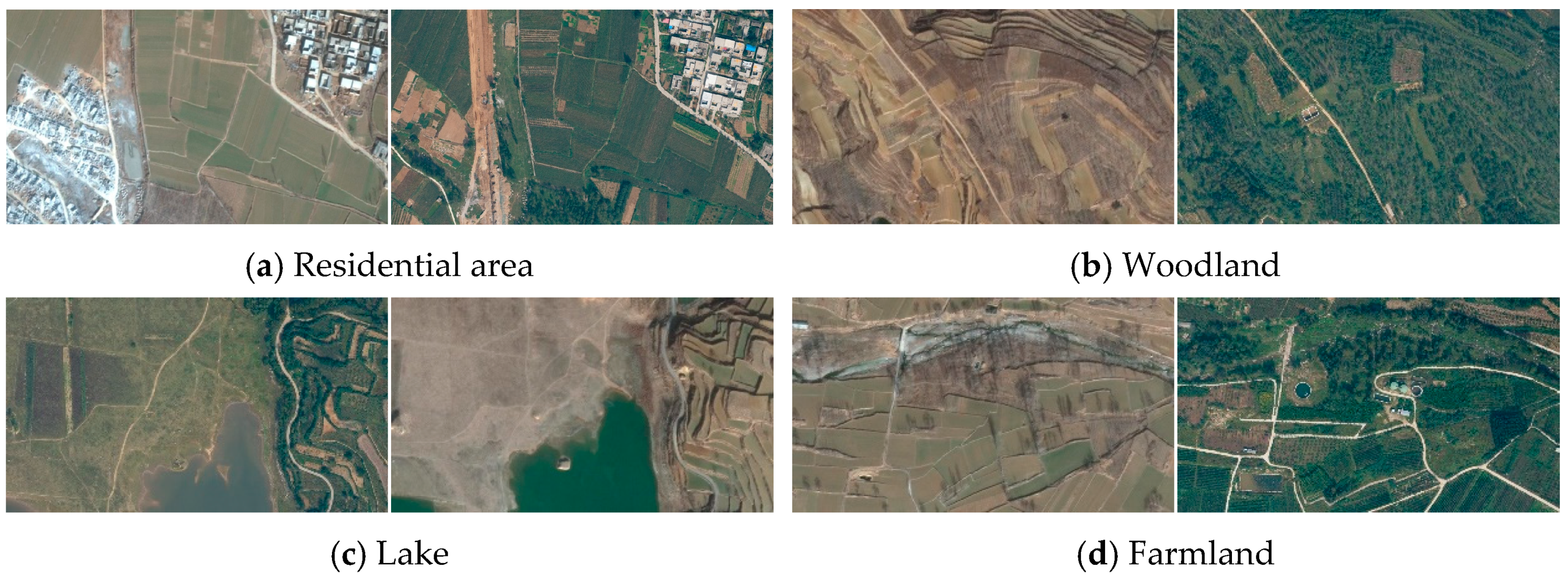
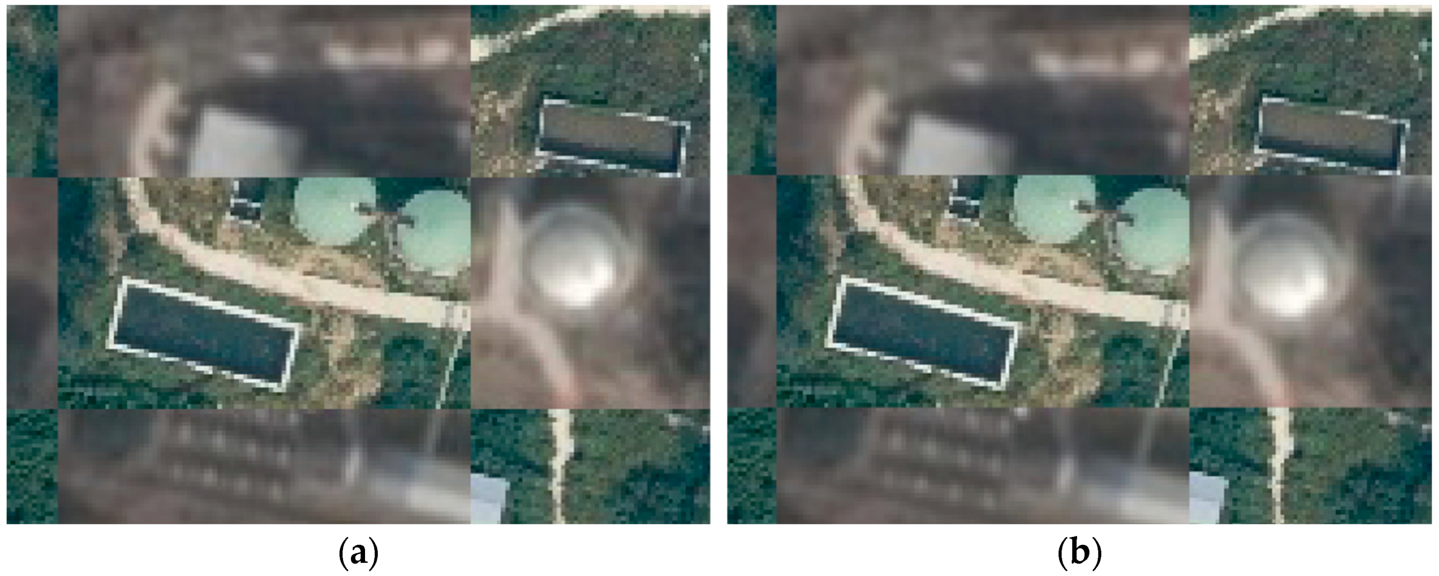
A method for building a training dataset of heterogeneous remote sensing images is suggested, and a dataset containing 700,000 pairs of images is generated for training and testing. Each image pair comprises pixel-level correspondence of UAV simulation images and satellite orthographic images. The dataset covers a period and obvious changes in the ground objects covering typical environments such as cities, suburbs, rural areas, and jungles. The original satellite images used to generate the dataset are available at https://drive.google.com/drive/folders/1EJIxYZthkN7GbfQNfdD1l8D5ADsl3WqX?usp=-sharing (accessed on 9 October 2022).
(3)
The Attention mechanism is visualized, and the differences between self-Attention and cross-Attention aggregation of the matched point pairs and unmatched points are analyzed by gradually deepening the network. Our analysis confirms the effectiveness of the Attention mechanism and studies the PRC curves of CSAM under different Attention layers to determine the optimal solution.
(4)
Comparative experiments are conducted against the NNDR, FSC, GMS, OA-Net, and SuperGlue algorithms on the test data set to verify the effectiveness of CSAM. A comparative experiment with RIFT and CFOG is also conducted on multimodal images to test the generalization ability of CSAM. Finally, a multimodal image registration experiment is conducted to test its efficiency for practical applications. The experiments highlight that CSAM has high robustness and efficiency. Therefore, it can provide a reasonable solution to heterogeneous remote sensing image matching.
The remainder of this paper is structured as follows. Section 2 introduces the Attention-based feature point matching method, CSAM, and elaborates on building a training dataset of heterologous remote sensing images. Section 3 explains the CSAM training based on the heterogeneous image training data and analyzes the process of Attention aggregation followed by comparisons with other existing methods. Finally, Section 4 summarizes the proposed method and presents several ideas for future studies.

2. Methodology

This section elaborates on the Cross and Self Attentional Matcher (CSAM), comprising: feature point encoding, feature aggregation, and matching optimization. In CSAM, the feature point position and descriptor are encoded, enabling the algorithm to exploit the context and surrounding point information during the feature aggregation process. Then, self-Attention and cross-Attention are used to aggregate the features. Furthermore, a linear attention mechanism reduces computational complexity and improves feature aggregation efficiency. Finally, a scoring matrix is established according to the features aggregated by the Attention mechanism, followed by the differentiable Sinkhorn algorithm that optimizes the matching based on a loss function to facilitate supervised learning. Section 2.2 further elaborates on the method of establishing the training dataset, including data sources, data characteristics, UAV simulation images, and satellite orthophoto correction.

2.1. The CSAM Architecture

The two images to be matched are A and B , each having a set of feature points p i and their corresponding feature descriptors d i . A and B have M and N feature points and descriptors, respectively. Also, x and y denote the horizontal and vertical coordinates of the feature points. The algorithm process is depicted in Figure 1.
Feature point encoding. Position encoding [45,52] is the first step in CSAM. To better represent the position information of the feature points p i , the horizontal and vertical axis coordinates x and y of the feature points’ positions are input into the multi-layer perceptron (MLP) for encoding. Then by splicing it with the feature descriptor d i , the initial feature vector ( 0 ) f i is obtained and input to the Attention network:
( 0 ) f i = d i + M L P p x i M L P p y i ,
where [ ] denotes concatenation.
Feature aggregation. The self-Attention and the cross-Attention layers are arranged alternately in the network for feature aggregation within and between the images. The initial feature vector ( 0 ) f i is input into the Attention network, and the feature aggregation of the self-Attention and cross-Attention layers is performed N times. The following equation represents the Attention information propagation of the i th feature vector of the image A at layer :
( + 1 ) f i A = ( ) f i A + MLP ( ) f i A m E i ,
where m E i denotes the process of attention aggregation [27,53]:
m E i = softmax 2 Q softmax 1 K T V ,   E E self   , E cross  
where Q , K , V n × d , n M , N , and d is the feature dimension. Each layer contains two secondary layers of self-attention and cross-attention. If E = E self , Q , K , V is the linear projection of all ( ) f i on the same image. Also, if E = E cross , Q is the linear projection of all ( ) f i on the image. Here, K , V are the linear projections corresponding to all ( ) f i on the image to be matched.
The input vectors of the Attention layer are usually referred to as query, key, and value. Similar to data retrieval, the query vector Q retrieves information from the value vector V according to the weight calculated by the dot product with the key vector K , where the value vector V and the key vector K are in one-to-one correspondence. The higher the similarity of Q to K , the more information is extracted from the corresponding V . As also illustrated in Figure 2a, the general Attention layer is defined as:
  Attention   ( Q , K , V ) = softmax Q K T V ,
In image matching, the number of features exceeds the feature dimension, i.e., n d . In (3) Q K T is an n × n matrix. Therefore, the complexity of the Attention mechanism is O n 2 [54]. Without Softmax, the Attention mechanism is the multiplication of three matrices Q K T V . Hence, using the associative law of matrix multiplication, we first obtain K T V , a d × d matrix, which is then left-multiplied by Q . Therefore, since d n , the complexity of the Attention mechanism is only O n . Here, this is presented by using the Linear Attention mechanism [54] (Figure 2b), which reduces the computational complexity by performing Softmax operations on Q , and K , respectively:
Attention   ( Q , K , V ) = softmax 2 Q softmax 1 K T V ,
where softmax 1 and softmax 2 denote the softmax operation in the first dimension n , and the second dimension d , respectively. Since Q is normalized in the second dimension d , and K is normalized in the first dimension n , Q K T is automatically normalized [54]. Hence, the complexity of the Attention mechanism is reduced from O n 2 to O n .
Matching optimization layer. We consider the inner product of the aggregated features ( N ) f i A and ( N ) f i B to obtain a scoring matrix S M × N . We note that a feature point has, at most, one matching point, while some feature points have no corresponding matching points. Therefore, we use the Sinkhorn algorithm [51,55] to optimize this matrix. The Sinkhorn algorithm is a differentiable Hungarian [56] algorithm that obtains the initial matching point pairs and their correspondences. Finally, the initial matching is filtered according to the preset threshold to obtain the final matching result.
As explained above, the entire algorithm is differentiable. Hence the algorithm can be trained by back-propagation. To supervise the training process, we consider the following loss function:
L = 1 M × N i = 0 M j = 0 N log ( S i j P i j ) ,
where P M × N is the real matching matrix obtained according to the transformation matrix between the two images and the feature points. The matching point assigns the corresponding position element in P to 0 according to the point number, while the other elements are set to 1.

2.2. Training Data Set

We consider an area of about 15 km2 near the Songshan Calibration Field in Dengfeng City, Henan Province, China. The established dataset contains 1,000,000 pairs of drone images and their corresponding satellite images. In this dataset, the images have a size of 540 × 960 pixels, and the training, validation, and test sets comprise 680,000, 10,000, and 310,000 image pairs, respectively. We consider this area because it covers a large variety of texture characteristics close to the Songshan Mountains’ undulating terrain, including typical environments such as woodland, farmland, residential area, water, and bare land.
The simulated UAV images are generated by setting different internal and external parameters using high-precision UAV orthophotos and elevation models. These were captured during the summer of 2018, and the ground resolution was consistent with the satellite images. The satellite orthophoto images were captured between 2009–2019 and covered four seasons with a ground resolution of 0.5 m published by Google Earth. Since the coordinates of the satellite orthophoto photos have a low accuracy of 5 m, a matching method based on position information is used for correction that corresponds to the pixel level of the UAV images. Figure 3 shows part of the image pairs of the dataset.

2.2.1. UAV Imagery

We set different internal and external parameters based on the high-precision UAV orthophoto images and elevation model. The iterative photogrammetric method [57,58] generates simulated images pixel-by-pixel. Starting from the simulated image and according to the parameters set, the coordinates of each element of the simulated image are obtained on the ortho-image using the single image mapping method. The corresponding gray interpolation and value obtained are illustrated in Figure 4.
The process is as follows. Let the pixel coordinate of a point in the simulated image be ( u s , v s ) . According to the inner orientation elements of the camera, the normalized plane coordinate ( x , y , 1 ) in the image space coordinate system is:
x = u s - c x f x y = v s - c y f y ,
where f x and f y are the normalized focal lengths on the u and v axes, respectively, and ( c x , c y ) denote the pixel coordinates of the camera’s optical center.
Given the exterior orientation elements of the camera and the elevation values of the corresponding ground point coordinates, the corresponding ground point plane coordinates are obtained using the collinearity equations:
X = Z Z S a 1 x + a 2 y a 3 c 1 x + c 2 y c 3 + X S Y = Z Z S b 1 x + b 2 y b 3 c 1 x + c 2 y c 3 + Y S ,
where ( X , Y , Z ) is the coordinate of the feature point corresponding to the ground point p in the geodetic coordinate system, and t = ( X S , Y S , Z S ) is the line element in the camera’s exterior orientation elements. Furthermore, a i , b i , c i ( i = 1 , 2 , 3 ) is the element in the rotation matrix R composed of the angle in the camera’s exterior orientation elements.
We note that the elevation value of the ground point coordinates is unknown, and only the DEM of the corresponding area is available. Therefore, it is necessary to iteratively solve the ground point coordinates using the monoscopic mapping method [59] (Figure 5), which allows for calculating the ground point coordinates corresponding to the simulated image points. Then, the image point coordinates on the orthophoto are obtained according to the plane coordinates of the ground points and the geographic parameters of the orthophoto. Nevertheless, the coordinates do not necessarily fall exactly at the center of the image element. Therefore, we use grayscale interpolation and the bilinear algorithm to address this issue.

2.2.2. Satellite Orthophoto

The considered satellite images are orthophotos published by Google Earth. The low precision of the plane coordinates of the satellite orthophoto image was corrected using a matching method based on position information, establishing pixel-level correspondence with the UAV orthophoto image. The correction process is depicted in Figure 6.
Here, the satellite orthophoto is first matched with the high-precision UAV orthophoto, and then the transformation matrix between the images is estimated. We use the CMM-Net [27] network for feature extraction and the NNDR algorithm for matching. The original location information is also used as a constraint to improve the probability of correct matching. After obtaining the matching pairs, RANSAC estimates the homography matrix between the images. The coordinates on the original satellite image are obtained for the corrected image according to the homography matrix, and finally, the grayscale interpolation and grayscale assignment are followed by the bilinear interpolation method. An instance of the images before and after the correction is illustrated in Figure 7, highlighting that even if the time between the two images is long and the buildings and vegetation significantly change, the correction algorithm can still grasp the invariant elements and achieve pixel-level correspondence.

3. Experiments

The experiments illustrate the training process of the CSAM algorithm and visualize the Attention module (Section 3.1). The conducted experiments under different Attention network layers are presented in Section 3.2 to determine the optimal number of layers. In Section 3.3, a comparative experiment is conducted involving multiple image-matching algorithms. To further test the CSAM’s performance, a multimodal image-matching experiment is conducted in Section 3.4. Finally, in Section 3.5, a registration experiment is carried out using multimodal images to test our method’s practical application effect in image registration. The hardware setup for the experiment involves the Ubuntu 20.04 operating system with an Intel i9-11900K CPU and a memory size of 64 GB. The graphic card is GeForce RTX 3090, and the algorithm is implemented in Python. The hardware requirements are not essential and can be replaced with other products.

3.1. Training and Visualizing the Attention

The CSAM algorithm initializes the weights by random numbers generated through a Gaussian distribution [60]. The Adam optimizer [61] is then used with an initial learning rate of 0.0001. We train CSAM for 300 epochs and decay the learning rate by an exponential 0.9998 every 20 epochs starting from the 100th epoch. To extract features, the Superpoint [62] algorithm is used. During training, the feature extraction network freezes and is only used to propagate gradients without participating in training. Furthermore, to prevent over-fitting, adding Gaussian filtering, changing resolution, and doing certain rotations are used for data augmentation during the training process. To further illustrate the algorithm’s mechanism, the process of aggregating features using self-Attention and cross-Attention is visualized in Figure 8 and Figure 9.
Figure 8 and Figure 9 show that the cross-Attention and self-Attention initially focus on the feature points of the whole image. As the number of network layers increases, the cross-attention of the correctly matched point pairs gradually changes to focusing on the corresponding matching points. The self-attention gradually focuses on the surrounding reliable points, and the distribution of Attention gradually becomes similar, resulting in more similar aggregated features of these two points and scores higher in the matching matrix.
For the unmatched points that need to be matched, the last layer of cross-Attention does not focus on the unmatched points. Although the two self-Attention modules gradually focus on the surrounding reliable points, the distribution of Attention is not similar. This makes the features of the two points aggregate differently and score lower in the matching matrix. The attention network increases the similarity of the matching points and the difference between unmatched points through context-based feature aggregation. It also initially realizes the correspondence between matching points and eliminates incorrect matching points.

3.2. Experiments with Attention Network Layers

The algorithm’s performance is evaluated using the precision vs. recall curve (PRC) [9,63]. The vertical axis of the curve is precision, which represents the proportion of correct matching to all matching, and the horizontal axis is recall, representing the proportion of correct matching in actual matching. The formulas for calculating recall and precision are:
Recall = N C M N C M + N F C M ,
Precision = N C M N C M + N F M ,
where NCM is the Number of Correct Matches, and NFM denotes the Number of False Matches. Also, NFCM is the number that could have been correctly matched but was missed by the algorithm. The farther the PRC curve is from the origin, the greater the recall and precision and the higher the algorithm’s performance.
The judgment formula for the correct matching point pair is:
H 1 f x 1 , y 1 x 2 , y 2 2 T ,
where x 1 , y 1 and x 2 , y 2 are the coordinates of the feature points of the simulated UAV image and the coordinates of the feature point of the satellite orthographic image, respectively. f represents the transformation from the coordinates of the simulated UAV image to the coordinates of the UAV orthographic image, and H is the homography matrix for correcting the satellite orthophoto image. Moreover, T is a threshold set as T = 3 2 pixels. The processing time (PT) (in seconds) is also used to evaluate the algorithm’s efficiency. The smaller the PT value, the higher the detector efficiency.
The test data set is used for matching experiments to analyze the impact of the number of Attention network layers on the matching algorithm. Figure 10 illustrates the performance of the matching algorithm with different Attention network layers. Subplots (a) and (b) correspond to the average PRC curve and average processing time of the images in the test dataset, respectively. Different recall and precision values are obtained by adjusting the threshold of the matching optimization layer. In our experiment, we set the thresholds to 0, 0.2, 0.4, 0.6, and 0.8. Figure 10 reveals that as the number of network layers increases and the PRC curve gradually moves away from the origin. When increasing the number of layers beyond 11, the curve position hardly changes, while the PT gradually increases. Considering the PRC curve and PT, we set the number of layers to 11 as the optimal number for the Attention network.

3.3. Comparison Test for Different Algorithms

To evaluate the effectiveness of CSAM, experiments are designed to compare it with the Superglue, NNDR + FSC, NNDR + GMS, OA-Net, SIFT, RIFT, and CFOG algorithms. For the feature points extracted by the SIFT and RIFT algorithms, the NNDR strategy is used to determine the initial matching point pairs, and the FSC algorithm is used to eliminate false matches. The NNDR + FSC, NNDR + GMS, OA-Net, Superglue, and CSAM algorithms perform matching and false matching elimination based on the feature points extracted by Superpoint. The considered test data is part of the test data set presented in Section 2.2. The corresponding test results are presented in Table 1 and Figure 11, Figure 12, Figure 13 and Figure 14, while the quantitative evaluation indicators include NCM, precision, and PT.
Table 1 highlights that among the eight algorithms evaluated, SIFT + NNDR + FSC, Superpoint + NNDR + FSC, Superpoint + NNDR + GMS, and Superpoint + OA-Net have a rather poor effect, low precision, and provide few correct matching point pairs. There are also many mismatches in the results obtained by Superpoint + Superglue. Compared with Superpoint + Superglue, Superpoint + CSAM achieves higher precision and more correct matching point pairs, and the algorithm takes the same time. This highlights that the proposed feature point encoding method can more effectively use the relative positional relationship between the feature points to aggregate features. The linear Attention mechanism ensures that the calculation amount of the algorithm remains unchanged by increasing the number of network layers. Considering RIFT + NNDR + FSC, CFOG, and Superpoint + CSAM, these all have higher precision, but the combination of Superpoint + CSAM has more correct matches and lower processing complexity. By comprehensively analyzing the three indexes of NCM, precision, and PT, the above results confirm that the CSAM algorithm outperforms the competitor methods on the test dataset.
Figure 11, Figure 12, Figure 13 and Figure 14 illustrate the matching effects of the four well-performing algorithms. The left image is a satellite orthographic image, and the right is a simulated UAV image. In these figures, subplots (a) and (c) are the images of the same sparse texture area, and (b) and (d) show images of the same area with relatively richer textures.
Compared with (a) and (b), the UAV images of (c) and (d) are rotated and tilted to a certain extent. Moreover, RIFT + NNDR + FSC, CFOG, and Superpoint + Superglue are less effective in areas with sparse or repeated textures, e.g., farmlands and woodlands, whereas more points are matched in densely textured residential areas. Furthermore, RIFT + NNDR + FSC and Superpoint + Superglue have certain anti-rotation and tilt capabilities. Moreover, Superpoint + Superglue can match more points. Nevertheless, there are also many mismatches and low precision. Finally, Superpoint + CSAM can match many matching points in different situations, and the distribution is relatively uniform.

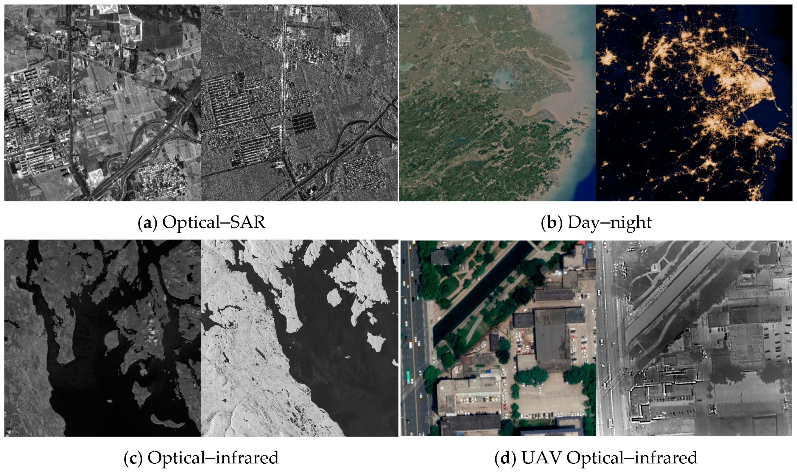
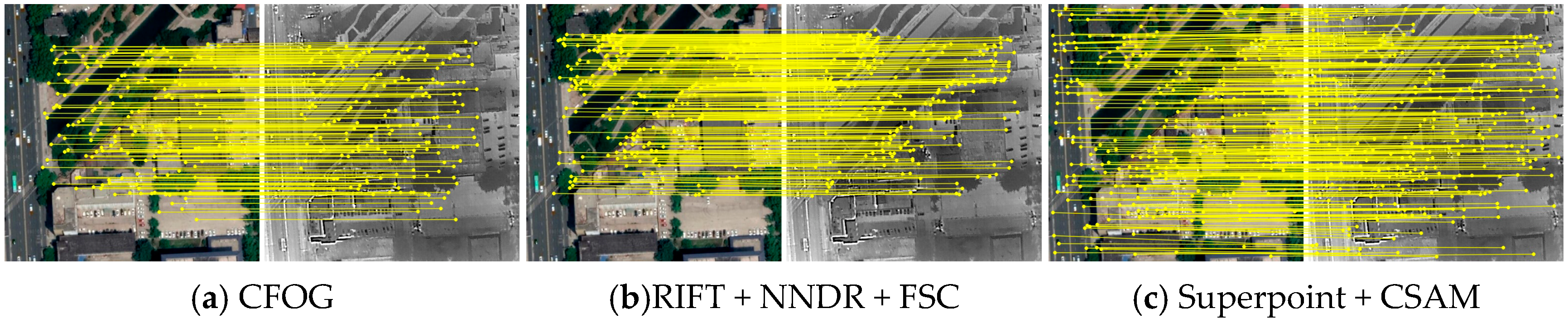
3.4. Multimodal Image Matching

A multimodal image-matching experiment is designed to evaluate the algorithm’s performance further. Since the algorithm is only trained on the visible light image dataset, the multimodal image-matching experiment can test the generalization ability of the algorithm on different bands and different types of images.
The competitor algorithms are RIFT + NNDR + FSC and CFOG, which perform better on the test dataset. The test data are presented in Table 2, and Figure 15, and the test data bands and modes include visible light, thermal infrared, SAR, luminous remote sensing images, grid maps, and depth maps. The test results are presented in Table 3 and Figure 16, Figure 17, Figure 18, Figure 19, Figure 20 and Figure 21. The evaluation index is NCM, and the judgment formula for correctly matched point pairs is:
H x 1 , y 1 x 2 , y 2 2 T ,
where x 1 , y 1 and x 2 , y 2 are the coordinates of the reference image feature points and the coordinates of the image feature points to be matched, respectively. Also, H is a homography matrix describing the projective transformation between two images, calculated by manually selecting 40–60 evenly distributed control points on the images. Here we also set T = 3 2 pixels.
Comparing and analyzing the results presented in Table 3 and Figure 16, Figure 17, Figure 18, Figure 19, Figure 20 and Figure 21 suggest the following. For Optical–SAR and Day–night image pairs, all three methods can correctly match a certain number of feature points, where RIFT + NNDR + FSC and Superpoint + CSAM both outperform CFOG. Nevertheless, for Optical–infrared image pairs with a certain rotation angle, CFOG completely fails. This is consistent with the performance in the test dataset. Superpoint + CSAM has more correct matching points than RIFT + NNDR + FSC and is more uniform.
The three methods can also match more feature points on Optical–map, UAV Optical–infrared, and Optical–map image pairs. However, the correct matching point pairs of CFOG and RIFT + NNDR + FSC are concentrated in the middle of the image, and the feature points at the edge of the image are not correctly matched. The correct matching point pair distribution of Superpoint + CSAM is more uniform.

3.5. Multimodal Image Registration

Image registration is one of the main purposes of image matching [8]. To illustrate the effectiveness of the CSAM algorithm, we conduct image registration experiments based on matching. First, the homography matrix is obtained according to the matching point group given by Superpoint + CSAM. This matrix is then used to correct the first image, and the corresponding image is registered with the second image. The effect of registration reflects the accuracy of the matching algorithm, and we use superimposed windowing for better illustration. Figure 22 shows the registration effect and partially enlarged diagrams of the four image groups. Except for the UAV Optical–infrared image, the registration errors of all regions on the other image types (modalities) are mainly controlled within 2 pixels. Additionally, some areas of the UAV Optical–infrared image are dislocated, which might be attributed to the drone’s low flying altitude and the tall buildings presented in the image. When the relative flight altitude is low, and the ground undulation is large, the ground can no longer be regarded as a plane. The homography matrix describes the mapping relationship between two planes and only applies to approximate planes. So the homography matrix cannot fit the transformation relationship between the two images.

3.6. Limitation Analysis

Although the proposed method is appealing, it also has two main limitations. First, CASM implements the image-matching process based on the feature points and descriptors extracted by Superpoint. However, Superpoint cannot handle heterogeneous images very well, and the repetition rate of the extracted feature points is low, decreasing matching precision. Second, in the matching process, CASM is not very sensitive to the absolute position accuracy of the feature points, and some matching points with large position differences cannot be eliminated. As shown in Figure 23, among the four matching point pairs in the partially enlarged image on the right, the positions of point pairs 1, 3, and 4 in both images are the same. However, the positions of the No. 2 point pair are different. In the case that there is no corresponding feature point in the same position as the two images, CASM selects the two points with the smallest error to form a matching pair.

4. Conclusions

This paper proposes a feature point matching method, CSAM, to achieve robust cross-modal image matching on heterogeneous remote sensing images. Our method relies on the Attention mechanism, and specifically, self-Attention and cross-Attention are alternatively used on the two images to be matched, exploiting feature point location and context information. The feature descriptor information is further aggregated, enabling CSAM to infer and eliminate the potential jointly and false matching points, respectively, and the Sinkhorn algorithm performs matching optimization. Furthermore, a method to build a training dataset of heterogeneous images has also been developed to improve the training efficiency. The dataset contains 1,000,000 image pairs generated for training, validation, and testing. Several experiments demonstrate that CSAM outperforms the competitor feature extraction and matching algorithms such as SIFT, RIFT, CFOG, NNDR, FSC, GMS, OA-Net, and Superglue, attaining an NCM and processing time of 183 and 0.13 s, respectively. While the average precision of CSAM is similar to that of RIFT and CFOG algorithms, its processing time is significantly lower. The experiments also reveal that CSAM has a strong generalization ability and robustness in matching and registering multimodal images. Compared with RIFT and CFOG, the matched points obtained by our method are more uniform, and the registration errors are mainly controlled within 2 pixels. Although CSAM affords robust matching between heterogeneous image feature points, the repetition rate of the feature points is relatively low because CASM is not very sensitive to the absolute position accuracy of feature points, and some matching points with large position differences cannot be eliminated. This is due to the Superpoint algorithm used to extract the feature points and descriptors in the CSAM training and experiment process. Thus, the low repetition rate of the feature points will decrease the matching precision. Therefore, future research must investigate more efficient source image feature extraction methods or devise end-to-end heterogeneous image matching algorithms based on CSAM.

Author Contributions

Conceptualization, H.H. and C.L.; methodology, H.H.; software, L.L. and F.Y.; validation, H.H., C.L. and Q.X.; formal analysis, H.H. and L.W.; resources, C.L.; writing—original draft preparation, H.H.; writing—review and editing, H.H., C.L. and X.X.; funding acquisition, C.L. and Q.X. All authors have read and agreed to the published version of the manuscript.

Funding

This work is supported by the Basic Research Strengthening Program of China (173 Program) (2020-JCJQ-ZD-015-00). It was also supported in part by the National Natural Science Foundation of China under grant nos. 42001338 and 42201492.

Data Availability Statement

The training data can be obtained from https://drive.google.com/drive/folders/1EJIxYZthkN7GbfQNfdD1l8D5ADsl3WqX?usp=sharing (accessed on 9 October 2022).

Acknowledgments

We are grateful to those involved in data processing and manuscript writing revision.

Conflicts of Interest

The authors declare no conflict of interest.

References

  1. Zhang, Y. Understanding image fusion. Photogramm. Eng. Remote Sens. 2004, 70, 657–661. [Google Scholar]
  2. Fang, Y.; Li, P.; Zhang, J.; Ren, P. Cohesion Intensive Hash Code Book Co-construction for Efficiently Localizing Sketch Depicted Scenes. IEEE Trans. Geosci. Remote Sens. 2021, 60, 5629016. [Google Scholar]
  3. Radke, R.J.; Andra, S.; Al-Kofahi, O.; Roysam, B. Image change detection algorithms: A systematic survey. IEEE Trans. Image Process. 2005, 14, 294–307. [Google Scholar] [CrossRef] [PubMed]
  4. Tuia, D.; Marcos, D.; Camps-Valls, G. Multi-temporal and multi-source remote sensing image classification by nonlinear relative normalization. ISPRS J. Photogramm. Remote Sens. 2016, 120, 1–12. [Google Scholar] [CrossRef] [Green Version]
  5. Brunner, D.; Lemoine, G.; Bruzzone, L. Earthquake damage assessment of buildings using VHR optical and SAR imagery. IEEE Trans. Geosci. Remote Sens. 2010, 48, 2403–2420. [Google Scholar] [CrossRef] [Green Version]
  6. Deren, L. Towards geo-spatial information science in big data era. Acta Geod. Cartogr. Sin. 2016, 45, 379. [Google Scholar]
  7. Jiang, X.; Ma, J.; Xiao, G.; Shao, Z.; Guo, X. A review of multimodal image matching: Methods and applications. Inf. Fusion 2021, 73, 22–71. [Google Scholar] [CrossRef]
  8. Ma, J.; Jiang, X.; Fan, A.; Jiang, J.; Yan, J. Image matching from handcrafted to deep features: A survey. Int. J. Comput. Vis. 2020, 129, 23–79. [Google Scholar] [CrossRef]
  9. Mikolajczyk, K.; Schmid, C. A performance evaluation of local descriptors. IEEE Trans. Pattern Anal. Mach. Intell. 2005, 27, 1615–1630. [Google Scholar] [CrossRef] [Green Version]
  10. Fischler, M.A.; Bolles, R.C. Random sample consensus: A paradigm for model fitting with applications to image analysis and automated cartography. Commun. ACM 1981, 24, 381–395. [Google Scholar] [CrossRef]
  11. Chum, O.; Matas, J.; Kittler, J. Locally optimized RANSAC. In Proceedings of the Joint Pattern Recognition Symposium, Madison, WI, USA, 18–20 June 2003; pp. 236–243. [Google Scholar]
  12. Wu, Y.; Ma, W.; Gong, M.; Su, L.; Jiao, L. A novel point-matching algorithm based on fast sample consensus for image registration. IEEE Geosci. Remote Sens. Lett. 2014, 12, 43–47. [Google Scholar] [CrossRef]
  13. Torr, P.H.; Zisserman, A. MLESAC: A new robust estimator with application to estimating image geometry. Comput. Vis. Image Underst. 2000, 78, 138–156. [Google Scholar] [CrossRef] [Green Version]
  14. Ni, K.; Jin, H.; Dellaert, F. GroupSAC: Efficient consensus in the presence of groupings. In Proceedings of the 2009 IEEE 12th International Conference on Computer Vision, Kyoto, Japan, 29 September–2 October 2009; pp. 2193–2200. [Google Scholar]
  15. Pilet, J.; Lepetit, V.; Fua, P. Fast non-rigid surface detection, registration and realistic augmentation. Int. J. Comput. Vis. 2008, 76, 109–122. [Google Scholar] [CrossRef]
  16. Ma, J.; Zhao, J.; Tian, J.; Bai, X.; Tu, Z. Regularized vector field learning with sparse approximation for mismatch removal. Pattern Recognit. 2013, 46, 3519–3532. [Google Scholar] [CrossRef]
  17. Ma, J.; Zhao, J.; Tian, J.; Yuille, A.L.; Tu, Z. Robust point matching via vector field consensus. IEEE Trans. Image Process. 2014, 23, 1706–1721. [Google Scholar] [CrossRef] [Green Version]
  18. Ma, J.; Zhou, H.; Zhao, J.; Gao, Y.; Jiang, J.; Tian, J. Robust feature matching for remote sensing image registration via locally linear transforming. IEEE Trans. Geosci. Remote Sens. 2015, 53, 6469–6481. [Google Scholar] [CrossRef]
  19. Ma, J.; Wu, J.; Zhao, J.; Jiang, J.; Zhou, H.; Sheng, Q.Z. Nonrigid point set registration with robust transformation learning under manifold regularization. IEEE Trans. Neural Netw. Learn. Syst. 2018, 30, 3584–3597. [Google Scholar] [CrossRef]
  20. Bian, J.; Lin, W.-Y.; Matsushita, Y.; Yeung, S.-K.; Nguyen, T.-D.; Cheng, M.-M. Gms: Grid-based motion statistics for fast, ultra-robust feature correspondence. In Proceedings of the IEEE Conference on Computer Vision and Pattern Recognition (CVPR), Honolulu, HI, USA, 21–26 July 2017; pp. 4181–4190. [Google Scholar]
  21. Ma, J.; Jiang, J.; Zhou, H.; Zhao, J.; Guo, X. Guided locality preserving feature matching for remote sensing image registration. IEEE Trans. Geosci. Remote Sens. 2018, 56, 4435–4447. [Google Scholar] [CrossRef]
  22. Ma, J.; Zhao, J.; Jiang, J.; Zhou, H.; Guo, X. Locality preserving matching. Int. J. Comput. Vis. 2019, 127, 512–531. [Google Scholar] [CrossRef]
  23. Jiang, X.; Ma, J.; Jiang, J.; Guo, X. Robust feature matching using spatial clustering with heavy outliers. IEEE Trans. Image Process. 2019, 29, 736–746. [Google Scholar] [CrossRef]
  24. Zhu, X.X.; Tuia, D.; Mou, L.; Xia, G.-S.; Zhang, L.; Xu, F.; Fraundorfer, F. Deep learning in remote sensing: A comprehensive review and list of resources. IEEE Geosci. Remote Sens. Mag. 2017, 5, 8–36. [Google Scholar] [CrossRef] [Green Version]
  25. Kussul, N.; Lavreniuk, M.; Skakun, S.; Shelestov, A. Deep learning classification of land cover and crop types using remote sensing data. IEEE Geosci. Remote Sens. Lett. 2017, 14, 778–782. [Google Scholar] [CrossRef]
  26. Liu, R.; Yang, C.; Sun, W.; Wang, X.; Li, H. Stereogan: Bridging synthetic-to-real domain gap by joint optimization of domain translation and stereo matching. In Proceedings of the IEEE/CVF Conference on Computer Vision and Pattern Recognition, Seattle, WA, USA, 13–19 June 2020; pp. 12757–12766. [Google Scholar]
  27. Sarlin, P.-E.; DeTone, D.; Malisiewicz, T.; Rabinovich, A. Superglue: Learning feature matching with graph neural networks. In Proceedings of the IEEE/CVF Conference on Computer Vision and Pattern Recognition, Seattle, WA, USA, 13–19 June 2020; pp. 4938–4947. [Google Scholar]
  28. Brachmann, E.; Krull, A.; Nowozin, S.; Shotton, J.; Michel, F.; Gumhold, S.; Rother, C. Dsac-differentiable ransac for camera localization. In Proceedings of the IEEE Conference on Computer Vision and Pattern Recognition, Honolulu, HI, USA, 21–26 July 2017; pp. 6684–6692. [Google Scholar]
  29. Ma, J.; Jiang, X.; Jiang, J.; Zhao, J.; Guo, X. LMR: Learning a two-class classifier for mismatch removal. IEEE Trans. Image Process. 2019, 28, 4045–4059. [Google Scholar] [CrossRef] [PubMed]
  30. Kluger, F.; Brachmann, E.; Ackermann, H.; Rother, C.; Yang, M.Y.; Rosenhahn, B. Consac: Robust multi-model fitting by conditional sample consensus. In Proceedings of the IEEE/CVF Conference on Computer Vision and Pattern Recognition, Seattle, WA, USA, 13–19 June 2020; pp. 4634–4643. [Google Scholar]
  31. Yi, K.M.; Trulls, E.; Ono, Y.; Lepetit, V.; Salzmann, M.; Fua, P. Learning to find good correspondences. In Proceedings of the IEEE Conference on Computer Vision and Pattern Recognition, Salt Lake City, UT, USA, 18–23 June 2018; pp. 2666–2674. [Google Scholar]
  32. Zhang, J.; Sun, D.; Luo, Z.; Yao, A.; Zhou, L.; Shen, T.; Chen, Y.; Quan, L.; Liao, H. Learning two-view correspondences and geometry using order-aware network. In Proceedings of the IEEE/CVF International Conference on Computer Vision, Seoul, Republic of Korea, 27–28 October 2019; pp. 5845–5854. [Google Scholar]
  33. Scarselli, F.; Gori, M.; Tsoi, A.C.; Hagenbuchner, M.; Monfardini, G. The graph neural network model. IEEE Trans. Neural Netw. 2008, 20, 61–80. [Google Scholar] [CrossRef] [PubMed] [Green Version]
  34. Zhao, X.; Zhang, J.; Yang, C.; Song, H.; Shi, Y.; Zhou, X.; Zhang, D.; Zhang, G. Registration for optical multimodal remote sensing images based on FAST detection, window selection, and histogram specification. Remote Sens. 2018, 10, 663. [Google Scholar] [CrossRef] [Green Version]
  35. Uss, M.; Vozel, B.; Lukin, V.; Chehdi, K. Efficient discrimination and localization of multimodal remote sensing images using CNN-based prediction of localization uncertainty. Remote Sens. 2020, 12, 703. [Google Scholar] [CrossRef] [Green Version]
  36. Dalal, N.; Triggs, B. Histograms of oriented gradients for human detection. In Proceedings of the 2005 IEEE Computer Society Conference on Computer Vision and Pattern Recognition (CVPR’05), San Diego, CA, USA, 20–26 June 2005; pp. 886–893. [Google Scholar]
  37. Ye, Y.; Bruzzone, L.; Shan, J.; Bovolo, F.; Zhu, Q. Fast and robust matching for multimodal remote sensing image registration. IEEE Trans. Geosci. Remote Sens. 2019, 57, 9059–9070. [Google Scholar] [CrossRef] [Green Version]
  38. Lowe, D.G. Distinctive image features from scale-invariant keypoints. Int. J. Comput. Vis. 2004, 60, 91–110. [Google Scholar] [CrossRef]
  39. Li, J.; Hu, Q.; Ai, M. RIFT: Multi-modal image matching based on radiation-variation insensitive feature transform. IEEE Trans. Image Process. 2019, 29, 3296–3310. [Google Scholar] [CrossRef]
  40. Xiong, X.; Xu, Q.; Jin, G.; Zhang, H.; Gao, X. Rank-based local self-similarity descriptor for optical-to-SAR image matching. IEEE Geosci. Remote Sens. Lett. 2019, 17, 1742–1746. [Google Scholar] [CrossRef]
  41. Shechtman, E.; Irani, M. Matching local self-similarities across images and videos. In Proceedings of the 2007 IEEE Conference on Computer Vision and Pattern Recognition, Minneapolis, MN, USA, 17–22 June 2007; pp. 1–8. [Google Scholar]
  42. Chaozhen, L.; Wanjie, L.; Junming, Y.; Qing, X. Deep learning algorithm for feature matching of cross modality remote sensing images. Acta Geod. Cartogr. Sin. 2021, 50, 189. [Google Scholar]
  43. Vaswani, A.; Shazeer, N.; Parmar, N.; Uszkoreit, J.; Jones, L.; Gomez, A.N.; Kaiser, Ł.; Polosukhin, I. Attention is all you need. Adv. Neural Inf. Process. Syst. 2017, 30. [Google Scholar] [CrossRef]
  44. Wang, H.; Zhu, Y.; Green, B.; Adam, H.; Yuille, A.; Chen, L.-C. Axial-deeplab: Stand-alone axial-attention for panoptic segmentation. In Proceedings of the European Conference on Computer Vision, Glasgow, UK, 23–28 August 2020; pp. 108–126. [Google Scholar]
  45. Carion, N.; Massa, F.; Synnaeve, G.; Usunier, N.; Kirillov, A.; Zagoruyko, S. End-to-end object detection with transformers. In Proceedings of the European Conference on Computer Vision, Glasgow, UK, 23–28 August 2020; pp. 213–229. [Google Scholar]
  46. Zhu, X.; Su, W.; Lu, L.; Li, B.; Wang, X.; Dai, J. Deformable detr: Deformable transformers for end-to-end object detection. arXiv 2020, arXiv:2010.04159. [Google Scholar]
  47. Dosovitskiy, A.; Beyer, L.; Kolesnikov, A.; Weissenborn, D.; Zhai, X.; Unterthiner, T.; Dehghani, M.; Minderer, M.; Heigold, G.; Gelly, S.J. An image is worth 16x16 words: Transformers for image recognition at scale. arXiv 2020, arXiv:2010.11929. [Google Scholar]
  48. Esser, P.; Rombach, R.; Ommer, B. Taming transformers for high-resolution image synthesis. In Proceedings of the IEEE/CVF Conference on Computer Vision and Pattern Recognition, Nashville, TN, USA, 20–25 June 2021; pp. 12873–12883. [Google Scholar]
  49. Lee, J.; Lee, Y.; Kim, J.; Kosiorek, A.; Choi, S.; Teh, Y.W. Set transformer: A framework for attention-based permutation-invariant neural networks. In Proceedings of the International Conference on Machine Learning, Long Beach, CA, USA, 10–15 June 2019; pp. 3744–3753. [Google Scholar]
  50. Velickovic, P.; Cucurull, G.; Casanova, A.; Romero, A.; Lio, P.; Bengio, Y. Graph attention networks. arXiv 2017, arXiv:1710.10903. [Google Scholar]
  51. Cuturi, M. Sinkhorn distances: Lightspeed computation of optimal transport. Adv. Neural Inf. Process. Syst. 2013, 26, 2292–2300. [Google Scholar]
  52. Gehring, J.; Auli, M.; Grangier, D.; Yarats, D.; Dauphin, Y.N. Convolutional sequence to sequence learning. In Proceedings of the International Conference on Machine Learning, Sydney, Australia, 6–11 August 2017; pp. 1243–1252. [Google Scholar]
  53. Gilmer, J.; Schoenholz, S.S.; Riley, P.F.; Vinyals, O.; Dahl, G.E. Neural message passing for quantum chemistry. In Proceedings of the International Conference on Machine Learning, Sydney, Australia, 6–11 August 2017; pp. 1263–1272. [Google Scholar]
  54. Shen, Z.; Zhang, M.; Zhao, H.; Yi, S.; Li, H. Efficient attention: Attention with linear complexities. In Proceedings of the IEEE/CVF Winter Conference on Applications of Computer Vision, Waikoloa, HI, USA, 4–8 January 2021; pp. 3531–3539. [Google Scholar]
  55. Sinkhorn, R.; Knopp, P. Concerning nonnegative matrices and doubly stochastic matrices. Pac. J. Math. 1967, 21, 343–348. [Google Scholar] [CrossRef] [Green Version]
  56. Munkres, J. Algorithms for the assignment and transportation problems. J. Soc. Ind. Appl. Math. 1957, 5, 32–38. [Google Scholar] [CrossRef]
  57. Linder, W. Digital Photogrammetry; Springer: Berlin/Heidelberg, Germany, 2009; Volume 1. [Google Scholar]
  58. Sheng, Y. Theoretical analysis of the iterative photogrammetric method to determining ground coordinates from photo coordinates and a DEM. Photogramm. Eng. Remote Sens. 2005, 71, 863–871. [Google Scholar] [CrossRef]
  59. Hou, H.; Xu, Q.; Lan, C.; Lu, W.; Zhang, Y.; Cui, Z.; Qin, J. UAV Pose Estimation in GNSS-Denied Environment Assisted by Satellite Imagery Deep Learning Features. IEEE Access 2020, 9, 6358–6367. [Google Scholar] [CrossRef]
  60. Brown, M.; Hua, G.; Winder, S. Discriminative learning of local image descriptors. IEEE Trans. Pattern Anal. Mach. Intell. 2010, 33, 43–57. [Google Scholar] [CrossRef] [PubMed] [Green Version]
  61. Kingma, D.P.; Ba, J. Adam: A method for stochastic optimization. arXiv 2014, arXiv:1412.6980. [Google Scholar]
  62. DeTone, D.; Malisiewicz, T.; Rabinovich, A. Superpoint: Self-supervised interest point detection and description. In Proceedings of the IEEE Conference on Computer Vision and Pattern Recognition Workshops, Salt Lake City, UT, USA, 18–23 June 2018; pp. 224–236. [Google Scholar]
  63. Gesto-Diaz, M.; Tombari, F.; Gonzalez-Aguilera, D.; Lopez-Fernandez, L.; Rodriguez-Gonzalvez, P. Feature matching evaluation for multimodal correspondence. ISPRS J. Photogramm. Remote Sens. 2017, 129, 179–188. [Google Scholar] [CrossRef]
Figure 1. The CSAM architecture.
Remotesensing 15 00163 g001
Figure 2. (a) Traditional Attention mechanism; (b) Linear Attention mechanism, where the rectangle size intuitively reflects the dimension of the matrix and the required amount of computations.
Remotesensing 15 00163 g002
Figure 3. Examples of the images in the dataset.
Remotesensing 15 00163 g003
Figure 4. UAV image generation process.
Remotesensing 15 00163 g004
Figure 5. Iterative photogrammetric algorithm [58].
Remotesensing 15 00163 g005
Figure 6. The correction process for the satellite orthophoto images.
Remotesensing 15 00163 g006
Figure 7. Comparing sample images before and after correction: (a) Overlay window of the original satellite orthophoto and UAV orthophoto; (b) Windowed overlay of the corrected satellite orthophoto and UAV orthophoto.
Remotesensing 15 00163 g007
Figure 8. Visualization of the Attention mechanism. We visualize an odd number of Attention layers, with cross-Attention on the left and self-Attention on the right. The yellow point is the correct matching, the green point denotes the incorrect matching point, the red line is the Attention of the target point on other points, and the color’s depth indicates the Attention’s intensity.
Remotesensing 15 00163 g008
Figure 9. Visualization of the last layer of the Attention for unmatched points. The points to be matched are obtained according to the maximum value of the cross-Attention of the last layer of the unmatched points. The visualization illustrates the distribution of two points on the graph and their Attention.
Remotesensing 15 00163 g009
Figure 10. The performance of the algorithm under different network layers.
Remotesensing 15 00163 g010
Figure 11. Partial matching results of RIFT + NNDR + FSC on the test dataset.
Remotesensing 15 00163 g011
Figure 12. Partial matching results of CFOG on the test dataset.
Remotesensing 15 00163 g012
Figure 13. Partial matching results of Superpoint + Superglue on the test dataset.
Remotesensing 15 00163 g013
Figure 14. Partial matching results of Superpoint + CSAM on the test dataset.
Remotesensing 15 00163 g014
Figure 15. Test image pairs.
Remotesensing 15 00163 g015aRemotesensing 15 00163 g015b
Figure 16. Optical–SAR matching results.
Remotesensing 15 00163 g016
Figure 17. Day–night matching results.
Remotesensing 15 00163 g017
Figure 18. Optical–infrared matching results.
Remotesensing 15 00163 g018
Figure 19. UAV Optical–infrared matching results.
Remotesensing 15 00163 g019
Figure 20. Optical–map matching results.
Remotesensing 15 00163 g020
Figure 21. Optical–LiDAR matching results.
Remotesensing 15 00163 g021
Figure 22. Image registration results and enlarged images.
Remotesensing 15 00163 g022
Figure 23. Distribution of feature points. The yellow point is the correct matching, and the green point denotes the incorrect matching point. On the right is a partially enlarged view of the same position in the two images.
Remotesensing 15 00163 g023
Table 1. Matching results of different algorithms on the test dataset.
Local FeaturesMatcherNCMPrecision (%)PT (s)
SIFTNNDR + FSC521.290.41
RIFT4381.2712.23
CFOGCFOG2683.653.19
SuperpointNNDR + FSC829.910.24
NNDR + GMS930.130.25
OA-Net610.122.60
Superglue3534.520.14
CSAM18381.290.13
Table 2. Description of test data.
CategoryReference ImageSensed ImageImage Characteristic
SensorGSDSizeSensorGSDSize
Optical-SARZY-3 PAN optical2.51000 × 1000CF-3 SL SAR31000 × 1000Different bands
Day–nightOptical-1000 × 1000SNPP/VIIS-1000 × 1000Day–night
Optical-infraredOptical-800 × 800Infrared-800 × 800Different bands with a certain rotation
Optical-infraredUAV Optical-512 × 512UAV Infrared-512 × 512Different bands with more details
Optical-mapGoogle Earth15500 × 500Open Street Map15500 × 500Different model
Optical-LiDARWorldView-2 optical2.0500 × 500LiDAR depth2.0500 × 500Different model
Table 3. The NCM of different methods.
CategoryCFOGRIFT + NNDR + FSCSuperpoint + CSAM
Optical–SAR16175251
Day–night2715872
Optical–infrared047358
UAV Optical–infrared135188233
Optical–map158349325
Optical–LiDAR148337269
Disclaimer/Publisher’s Note: The statements, opinions and data contained in all publications are solely those of the individual author(s) and contributor(s) and not of MDPI and/or the editor(s). MDPI and/or the editor(s) disclaim responsibility for any injury to people or property resulting from any ideas, methods, instructions or products referred to in the content.

