Fusion and Classification of SAR and Optical Data Using Multi-Image Color Components with Differential Gradients

Abstract

This paper proposes a gradient-based data fusion and classification approach for Synthetic Aperture Radar (SAR) and optical image. This method is used to intuitively reflect the boundaries and edges of land cover classes present in the dataset. For the fusion of SAR and optical images, Sentinel 1A and Sentinel 2B data covering Central State Farm in Hissar (India) was used. The major agricultural crops grown in this area include paddy, maize, cotton, and pulses during kharif (summer) and wheat, sugarcane, mustard, gram, and peas during rabi (winter) seasons. The gradient method using a Sobel operator and color components for three directions (i.e., x, y, and z) are used for image fusion. To judge the quality of fused image, several fusion metrics are calculated. After obtaining the resultant fused image, gradient based classification methods, including Stochastic Gradient Descent Classifier, Stochastic Gradient Boosting Classifier, and Extreme Gradient Boosting Classifier, are used for the final classification. The classification accuracy is represented using overall classification accuracy and kappa value. A comparison of classification results indicates a better performance by the Extreme Gradient Boosting Classifier.

1. Introduction

Image fusion techniques are aimed to obtain an improved single view with more information contents and preserving the spatial details by combining multimodal data obtained using different sources [1,2]. It has gained widespread attention for its efficiency in interpreting satellite images and as a tool for remote sensing image processing [2,3,4,5,6]. Satellite image fusion aids in geometric precision improvement, feature enrichment, and image sharpening [1,7,8,9,10]. A major application in the realm of remote sensing is to integrate these imageries (i.e., optical and SAR satellite images). Both of the remote sensing images are frequently widely used for a variety of remote sensing research. SAR data measures the physical characteristics of the ground objects and is independent of weather conditions, whereas optical data typically spans the wavelength region of electromagnetic radiation for near-infrared, visible, and short infrared [11,12]. The integration of optical and SAR images has widely been researched because of the very high spatial resolution SAR (Sentinel 1A), and optical satellite data (Sentinel 2B) is freely available and uses their complimentary information for image interpretation as well as classifications [13,14,15].

Within last few decades, various pixel-level image fusion algorithms have been proposed. However, these methods may result in low contrast with few improved details in the output image. Due to the human visual system’s (HVS) sensitivity to imaging features, multiple transformation techniques, such as multi-scale or multi-resolution transformations, which include contourlet transform, wavelet, and curvelet transform; contrast pyramids are also used [16,17,18]. Several studies also proposed gradient-based image fusion approaches to integrate images (i.e., visible and infrared). Ma et al. (2016) created a fusion approach for infrared and visible images utilizing total variation minimization as well as gradient transfer and found it performed well for infrared image sharpening [19]. Zhao et al. (2017) reported the fusion method using entropy coupled with gradient regularization to combine infrared as well as visible images [20,21]. Zhang et al. (2017) developed a method for the preservation of visual information and extracting image features [22,23]. Jiang et al. (2020) proposed a differential image gradient based fusion approach for visible and infrared images. In spite of their applications in image fusion, a major limitation of all these methods is that they have been applied for 2D images and these approaches cannot extract accurate spatial details from the images [24,25].

After the fusion, the classification of the fused images needs to be performed for further studies. One of the crucial studies employing remote sensing images is to discriminate land use and land cover classes using classification [8,26]. Out of various classification algorithms, machine learning classifications, including support vector machines, neural network, and random forest, have comprehensively been utilized by the community of remote sensing. Machine learning approaches often take a range of input predictors, may model complex class signatures, and never make any predictions about the distribution of the data. Numerous studies indicate that these approaches outperform conventional statistical classifiers in terms of accuracy, particularly for complicated data with a feature space of high-dimensional [27,28,29]. The classification of remote sensing images via approaches such as machine learning offers efficient and successful classification [30,31]. The superiority of these approaches includes their capability in handling data of high dimensionality and mapping the classes with extremely complicated properties. Various machine learning algorithms, including neural networks [32,33], decision trees [34,35], random forests [10,36], support vector machines [22,37], Stochastic gradient descent [38,39], and Stochastic Gradient Boosting [40], have been widely used with remote sensing images. These techniques make use of spectral data as inputs and may be able to achieve certain useful desired outputs through complex calculations [41]. Several articles on application of random forests (RFs) and support vector machines (SVMs) explored their feasibility for remote sensing imageries [7,10].

Within last two decades, Stochastic Gradient Descent (SGD) based classification approaches have drawn a considerable amount of attention and are recognized as an efficient strategy to discriminatory learning of linear models under convex loss functions [42,43]. Consequently, SGD-based approaches have been widely employed for registration, feature tracking, image registration, and image representation of satellite images [10,34,39,43,44,45,46].

Stochastic methods, including RF and SGB (Stochastic Gradient Boosting), offer higher prediction performance over parametric methods in several applications as well as for the particular datasets [47,48]. While SGB is indeed starting to acquire popularity in a variety of applications, RF has been widely employed in remote sensing and ecological applications [49]. A detailed literature review suggests only few applications of SGD and SGB classifier to classify remote sensing data. In addition, Extreme Gradient Boosting (or XGB) is a recently developed algorithm used for remote sensing applications [34,50,51,52].

In view of various limitations of the fusion methods and the advantages of SAR and optical data, an algorithm that combines the difference image; gradient image of color components in x, y, and z direction; and the magnitude of the gradients as well as the tensor components to deal with the spatial information is proposed for image fusion. The fusion results were evaluated using various fusion indicators with remote sensing images. Finally, the classification of fused images is performed using SGD, SGB, and XGB Classifier.

2. Materials and Methods

2.1. Study Area and Satellite Data

The main study area considered is the Central State Farm in Hissar region of Haryana, (India), which is situated at 29.2986°N and 75.7391°E latitudes. The crop fields are maintained at large scale on this substantial farmland for seed production and distribution to local farmers. The area’s main agricultural crops include pulses, maize, paddy, and cotton in kharif season and wheat, mustard, gram, sugarcane, and peas in rabi season. Figure 1 illustrates the False Color Composite (FCC) image of the considered study region.

The field visit of the testing site was undertaken on 6 April 2019 to collect the ground reference data for the study. After a visual examination of the Sentinel 1A/ 2B data along with the ground truth information, twelve different types of land cover were found, such as Fallow land, Built-up-area, Dense Vegetation, Fenugreek, Fodder, Gram, Mustard, Oat, Pea, Sparse Vegetation, Spinach, and Wheat. The Copernicus open access site was utilised to download the datasets for this study. Both the datasets from Sentinel 1A (S1) and Sentinel 2B (S2) were acquired on 23 and 24 March 2019, respectively. In the case of Sentinel 1A and Sentinel 2B, we used Level 1 data and Level 1-C data, respectively. Red, Green, Blue, and Infrared images from S1 (VV and VH) polarisation and S2 images with a 10 m spatial resolution were utilized. However, the reference image was created after visiting the study area on the ground. Due to the size of the farm in the area of study, ground reference data was created, taking into account their central location, giving each field a rectangular or square shape.

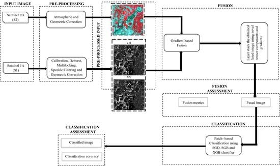
2.2. Proposed Methodology

A novel approach for image fusion is proposed to integrate the complimentary characteristics from both SAR (S1) and optical (S2) images. Figure 2 illustrates the detailed methodology applied for fusion and classification.

2.2.1. Preprocessing

The two input images S1 and S2 of size 964-pixel × 1028-pixel were extracted as a subset image for the considered study area using Sentinel Application Platform (SNAP) v6.0 (Figure 2). The preprocessing of S1 involves radiometric calibration, deburst operation, multi-looking, speckle noise reduction using Refined Lee filter, geo-referencing, and finally geometric correction. However, S2 involves geometric correction and atmospheric correction. Both S1 and S2 were resampled at 10m resolution for further processing that includes fusion and classification.

2.2.2. Fusion

Fusion of S1 and S2 images mainly involves the absolute difference of considered input images, Sobel-based gradients in x, y, and z direction, magnitude of the gradients’ color components, normalized component for the rate of change in the gradients, and finally fusion is applied to achieve the desired result. These steps are described as follows:

• Absolute Difference

The first step under fusion is the absolute difference of the input images (i.e., SAR (S1) and Optical (S2)). The absolute difference method helps to find the difference of input images S2 and S1 using corresponding pixels. The purpose of this method is to show the extent of changes between the two images as well as to remove the background variations for analyzing the foreground features.

The absolute difference method is initiated by subtracting the pixel reflectance spectra of S2 and S1 images by the following equation.

$$D=abs\left({{\displaystyle \sum }}_i^{4}S{2}_i-S1\right), for i=1,2,3,4$$

(1)

2.

Sobel-based gradient of the S1 and S2 image

Image gradients are generally the measure of image sharpness, and it represents the derivative of the energy recorded in the Digital Number (DN) values of neighboring pixels. The image gradient techniques may also specify the intensity as well as changes in the texture and color in a particular direction. To extract the gradient of the images, various operators for edge detection, such as Sobel, Canny, etc., can be used. In this paper, Sobel operator, which is found to have better performance in image gradient calculation, is used. The Sobel operator analyzes a 2D spatial gradient on an image and focuses more on edges and regions with a significant spatial gradient. For this study, the Sobel operator with a 3 × 3 size mask is used because a lager mask size may lead to the remove the small details of an image.

The gradient method was used to extract complementary information obtained from S1 and S2 images as well as to extract the boundaries of the ground truth classes very precisely. The differential image gradient of from Sentinel 1A/ B and Sentinel 2A/ B image is defined after introducing I_z gradient value in the following equation.

$$\nabla I=\left(I_x, I_y, I_z\right)$$

(2)

where $I_x$, $I_y$, and $I_z$ are the values of gradient for respective four bands in the x, y, and z (i.e., z+1 direction), respectively.

$$I_x=S_x.\ast \left(D_i\right)$$

(3)

$$I_y=S_y.\ast \left(D_i\right)$$

(4)

$$I_z=S_z.\ast \left(D_i\right)$$

(5)

where $S_x, S_y, \mathrm{and} S_z$ are components of Sobel operator in x, y, and z (i.e., z + 1 direction) and $\ast$ represents the convolution operator.

3.

Color components of the gradients in x, y, and z direction

The image gradient space includes some high-level discriminative data and characteristics in comparison to conventional RGB color space [40]. In this study, color components of the gradients for four multi spectral bands including Red (R), Green (G), Blue (B), and Near Infrared (NIR) from S2 image have been considered. The color components [37] for S2 image can be defined as R (x, y, z), G (x, y, z), B (x, y, z), and NIR (x, y, z). Therefore, the whole image is defined by the function f = (R, G, B, NIR). The unit vectors (i.e., $r$, $g$, $b$, and $nir$) was introduced and are associated with respective R, G, B, and NIR axes. These vectors f_m, m = 1, 2, 3 can be defined in the following manner.

$$u=I_{x1}\left(r\right)+I_{x2}\left(g\right)+I_{x3}\left(b\right)+I_{x4}\left(nir\right)$$

(6)

$$v=I_{y1}\left(r\right)+I_{y2}\left(g\right)+I_{y3}\left(b\right)+I_{y4}\left(nir\right)$$

(7)

$$w=I_{z1}\left(r\right)+I_{z2}\left(g\right)+I_{z3}\left(b\right)+I_{z4}\left(nir\right)$$

(8)

where, $I_{x1}$, $I_{x2}$,$I_{x3}$, $I_{x4}$, $I_{y1}$, $I_{y2}$,$I_{y3}$, $I_{y4}, I_{z1}$, $I_{z2}$,$I_{z3}$, and $I_{z4}$ are the gradients of R, G, B, and NIR color components obtained from Equations (3)–(5). The variables $u$, $v$, and $w$ are the function of three space coordinate x, y, and z.

In addition, divergence of the gradient, $Div$, is calculated using the Equations (6)–(8) in x, y, and z direction.

$$Div=\overrightarrow{u}+\overrightarrow{v}+\overrightarrow{w}$$

(9)

where, Div is the divergence of the gradients.

4.

Applying fusion rule for SAR and optical image

The absolute difference calculated in Equation (1) cannot be superimposed directly over the S2 image because it may lead to the larger pixel values of S2 image that may further lead to a brighter image. The brighter image may suppress the features of the image including texture, intensity, color, and boundaries. Therefore, the following equation is applied.

$$F_0=\{ \begin{array}{c}\left(\frac{S2}{\mathrm{ß}}\right)+D_i, S2>S1\\ \frac{ S2}{2}, others\end{array}$$

(10)

where $F_0$ is the first fusion and ß is the factor of suppression and is not influenced by any other parameters. The suppression factor ß = 10 has been taken to suppress the large values of the S2 image.

5.

Obtain final gradient image using gradient color components

To obtain the final gradient image, Equations (6)–(8) are considered. The dot product of the $u$, $v$, and $w$ is calculated using the following equation:

$$g_{xx}=u\times u$$

(11)

$$g_{yy}=v\times v$$

(12)

$$g_{zz}=w\times w$$

(13)

$$g_{xy}=u\times v$$

(14)

where g_xx$\left(g_{11}\right)$, g_yy$\left(g_{22}\right)$, g_xy$\left(g_{12}\right)$, g_zz$\left(g_{33}\right)$, respectively, are the tensor components, which are the functions for the space coordinates x, y, and z direction. From a mathematical point of view, the gradient of the multi-images (f) is a tensor g, f denoted as a vector field for the x, y, and z plane. Therefore, its gradient should be a tensor.

The subsequent equation can be utilized to compute the direction of the gradient function’s highest rate of change for a specific direction [53].

$${\mathsf{\theta }}_{\left(x,y,z\right)}=\frac{1}{2}ta{n}^{-1} \{ 2 (g_{xy} (1-\alpha )-g_{xz} (\mathrm{ß}-\mathrm{\gamma })+2g_{yz}\mathrm{\zeta }/(g_{xx}+g_{yy}+g_{zz}+4g_{yz}\mathrm{ß}))\}$$

(15)

where, $\mathsf{\alpha }=\cos 4\mathsf{\theta }/\cos 2\mathsf{\theta }$, $\mathrm{ß}=\cos \mathsf{\theta }$, $\mathsf{\gamma }=\cos 3\mathsf{\theta }/\cos 2\mathsf{\theta }$, $\mathsf{\zeta }=\sin \mathsf{\theta }/\cos 2\mathsf{\theta }$.

After calculating ${\mathsf{\theta }}_{\left(x,y,z\right)}$, $F_{\theta }$ is calculated by introducing g_zz to obtain the maximum directional change in the intensity for the fusion.

$$\begin{gathered} F_{\mathsf{\theta }\left(x,y,z\right)}=\left[ \frac{1}{2} \left(g_{11}si{n}^2\left(\mathsf{\theta }\right)+g_{22}si{n}^4\left(\mathsf{\theta }\right)+g_{33}co{s}^2\left(\mathsf{\theta }\right)+g_{12} si{n}^2\left(\mathsf{\theta }\right)\cos 2\mathsf{\theta }+ \\ {g}_{23} sin\mathsf{\theta } \cos 2\mathsf{\theta }+2g_{13} sin2\mathsf{\theta } \cos \mathsf{\theta }\right)\right]{ }^{1/2} \end{gathered}$$

(16)

where $F_{\theta \left(x,y,z\right)}$is the equivalent in size to the input colour image and can be interpreted as a gradient image. The produced gradient image would draw attention to important texture elements like lines, corners, and curves.

6.

Obtaining final fused image

Finally, to fuse image of S1 and S2 images, the following equation is used.

$$F_1=F_0+div+F_{\theta }$$

(17)

where, $F_1$is the fused result retaining their true values. The divergence has been added to F₀ in Equation (10) so that the pixel value may not scale down when the class boundaries are enhanced.

$F_1$ obtained from Equation (17) had some lesser pixel values with low brightness. Therefore, to restore the pixel details of S2 and S1 images, S2 is compared with F1 that can also extract the important features such as texture, color, and brightness of S1 image. The following equation is used for the above-mentioned purpose.

$$F_2=\{\begin{array}{c} S2, S2> F_1\\ F_1, others\end{array}$$

(18)

where, $F_2$is the result after applying contrast to the S2 image. The final fused result is obtained after applying the following equation.

$$F_3=abs\left(F_2-div\right)$$

(19)

where, $F3$ is fused result and final fused image is formed by layer stacking of all four bands fused images.

2.2.3. Classification

• Stochastic Gradient Descent (SGD) Classifier

Stochastic Gradient Descent (SGD) is a simple supervised discriminative learning with convex loss functions using linear classifiers. With more than 10^5 training samples and features, this classifier can handle very big matrices. By integrating many binary classifiers using the one versus all (OVA) approach, SGD Classifier provides multiclass classification [51], and requires parameter tuning to find the best classification results. When dealing with large scale data of a variety of classes, SGD classifiers have been found to perform more accurately in a few published applications using remote sensing images [7,36].

2.

Stochastic Gradient Boosting (SGB) Classifier

The machine learning approach (i.e., SGB) integrates the advantages of boosting and bagging techniques [40]. A decision tree also known as simple base learner is specifically created for each SGB iteration by sub-sampling the training dataset randomly (with no replacement), resulting in significant increases to the model’s performance. The steepest gradient technique serves as the foundation to boosting the processing in the SGB model, which gives more focus on wrongly selected training pixels, that are close to their accurate classification than on the lowest-quality classification [54]. Low sensitivity to outlier effects, the ability to deal with incorrect training datasets, stochastic modeling of non-linear relationships, resilience in handling interactions between predictors, and the capacity to evaluate the value of variables individually are several major advantages of the SGB classifier [42]. Additionally, the SGB algorithm’s stochastic component is a valuable tool for enhancing classification accuracy and minimizing overfitting [40].

3.

Extreme Gradient Boosting (XGB) Classifier

It is a concurrent tree boosting approach that provides more accurate large-scale issue solving. With XGB, a classifier built from gradient boosting where weak tree classifiers are iteratively concatenated to create a strong classifier. XGB classifier is used to optimize the loss function while constructing the iterative model and the new aspect of XGB is to include an objective function that makes use of a regularization term for managing the complexity of the model with the loss function [34]. This allows for the continuation of optimal processing speed and parallel calculations. In this study, the softmax multiclass classification as an objective function was employed. Using the function Softmax, each class is normalized into a probability distribution with a range of (0, 1) that adds up to 1. XGB is described mathematically in great depth by Chen and Guestrin [34]. In a few applications using remote sensing images, the usage of XGB has been described. It has been reported to provide improved accuracy while handling large-scale data composed of multiple classes [30,46]. In this work, XGB is taken into consideration for the classification of the obtained fused images due to its outstanding scalability and effectiveness with remote sensing images [38,46].

To classify fused, layer stacked (S2 and S1 (VV, VH) separately), and S2 datasets used in this study, patch-based approach for classification was used. Using an image patch instead of individual pixels provides the use of the spatial and spectral characteristics of the pixels while classification. In a patch-based classifier, a pixel’s spatial characteristics are determined by its nearby pixels in a fixed-size window (i.e., image patch). Ground reference images were used to extract image patches of various sizes (say, 3 × 3) for both S1 and S2 images for training and testing of all considered classifiers (SGB, SGD, and XGB). Every class is allocated a number in ground truth image and areas with absence of class information are allocated a zero value. When a patch extraction of size 3 is performed, only those image patches with a central pixel with a non-zero value were taken into consideration throughout classification. The overall number of train and test samples to classify S2, fused S2 with S1 (VH and VV), and non-fused fused S2 with S1 (VH and VV) images are listed in

Table 1. Total samples used for training and testing in S2, fused S1 and S2 images.

Class Number	Class Name	Training Samples	Testing Samples
1	Fallow land	663	221
2	Built-up-area	1376	459
3	Dense Vegetation	217	72
4	Fenugreek	126	42
5	Fodder	85	28
6	Gram	533	178
7	Sparse Vegetation	2058	686
8	Wheat	773	258
9	Mustard	310	103
10	Oat	337	112
11	Pea	371	124
12	Spinach	179	60

.

For fusion, MATLAB 2019b and for classification, scikit-learn and Keras with Tensorflow were used.

3. Results

This section provides the fusion and classification results for S1 and S2 images using the approaches described in Section 2.

3.1. Fusion

Table 2. Assessment of the Fusion Metrics of Hissar, Haryana (India).

Fusion Approach	Polarization	Fusion Metric
		ERGAS	SAM	UIQI	SSIM	CC	RASE	PSNR
KLT	VH	54.17	126.28	−1.63	4.49	0.01	−175.9	−49.02
	VV	56.32	131.6	3.09	4.48	0.05	−165.91	−53.96
GIV	VH	6.04	4.94	0.79	0.47	0.96	24.17	36.47
	VV	5.75	4.16	0.83	0.79	0.97	22.98	38.56
Proposed	VH	6.62	2.94	0.86	0.78	0.98	26.47	38.27
	VV	6.01	3.11	0.88	0.85	0.98	24.05	39.80

provides the results of numerous metrics used to assess different fusion methods after applying fusion over S2 and S1 (VV and VH polarization) satellite data [12].

Fusion metrics [12] were considered such as Erreur Relative Globale Adimensionnelle de Synthese (ERGAS), Spectral Angle Mapper (SAM), Relative Average Spectral Error (RASE), Universal Image Quality Index (UIQI), Structural Similarity Index (SSIM), Peak Signal-to-Noise Ratio (PSNR), and Correlation Coefficient (CC). The fusion metrics are as follows:

(1)

Erreur Relative Globale Adimensionnelle de Synthese (ERGAS) calculates the quality in terms of normalized average error of the fused image. A higher value of ERGAS indicates distortion in the fused image whereas lower value indicates similarity of the reference and fused images.

(2)

Spectral Angle Mapper (SAM) computes the spectral angle between the pixels, vector of the reference image, and fused image. A lower value of SAM closer or equal to zero indicates the absence of spectral distortion.

(3)

Relative Average Spectral Error (RASE) represents the average performance in the spectral bands where the lower value of RASE indicates higher spectral quality of the fused image.

(4)

Universal Image Quality Index (UIQI) computes the data transformation from reference image to the fused image. Range of this metric is −1 to 1 and the value close to 1 indicates the similarity of the reference and fused images.

(5)

Structural Similarity Index (SSIM) compares the local patterns of pixel intensities of the reference and fused images. Range of this metric varies from −1 to 1 and the value closer to 1 indicates similarity of the reference and fused images.

(6)

Peak Signal-to-Noise Ratio (PSNR) is calculated by dividing the corresponding pixels of the fused image with the reference. A higher value of this metric indicates superior fusion that suggests the similarity of the reference and fused images.

(7)

Correlation Coefficient (CC) computes the similarity of spectral features between the reference and fused images. The value closer to 1 indicates the similarity of the reference and fused images.

Assessment of the results of gradient based fusion (GIV) [24], KL (Karhunen-Loeve) transform based fusion (KLT) [25] and proposed gradient based fusion approach suggests better performance by proposed gradient based fusion approach (Table 2). The results suggest poor performance by KLT approach in terms of various fusion metrics (Table 2).

Figure 3 and Figure 4 displays the fused images created by GIV and proposed approach only, such as S2 fused with distinct VH and VV polarized images of S1 data, to allow for visual comparison of the effectiveness of the various fusion approaches under consideration. The obtained images after fusing S2 with S1 (VH and VV polarization separately) are shown using three spectral bands (G, R, and NIR; Figure 3 and Figure 4).

3.2. Classification

To assess the effectiveness of the fused satellite images using the resultant classification accuracy, different classification approaches were performed using SGD, SGB, and XGB classifiers. Kappa value and overall classification accuracy for fused images obtained by the proposed fusion approach are provided in

Table 3. Classification Result of SGD, SGB and XGB Classifier.

Classification Approach with Patch Size = 3	Polarization	Accuracy Measure
		Overall Accuracy (%)	Kappa Value
SGD	VH	71.16	0.65
	VV	71.39	0.66
SGB	VH	91.42	0.89
	VV	91.89	0.90
XGB	VH	93.72	0.92
	VV	94.75	0.93

.

The fused image obtained by the proposed fusion approach is also compared with various non-fused images using XGB classifier in

Table 4. Classification Result of Sentinel 2B (S2), Sentinel 2B (S2) layer stacked with Sentinel 1A (S1;VV) and Sentinel 2B (S2) layer stacked with Sentinel 1A (S1; VH) using XGB Classifier.

XGB Classifier with Patch Size = 3	Accuracy Measure
	Overall Accuracy (%)	Kappa Value
S2	88.49	86.25
S2 layer stacked with S1 (VV)	90.01	88.08
S2 layer stacked with S1 (VH)	89.43	87.38

.

The class-wise accuracy in

Table 5. Class-wise accuracy for Sentinel 2B (S2), S2 layerstacked with VH-VV polarization separately (i.e., S2 + VH and S2 + VV), and fused image by proposed fusion approach using XGB classifier.

Class Name	Overall Accuracy (%)
	S2	S2 + VH	S2 + VV	Proposed Approach
				VH	VV
Fallow land	93.00	93.00	95.00	94.00	96.00
Built-up-area	99.00	99.00	99.00	100.00	100.00
Dense Vegetation	86.00	93.00	89.00	88.00	97.00
Fenugreek	38.00	38.00	61.00	56.00	62.00
Fodder	59.00	73.00	62.00	91.00	91.00
Gram	81.00	82.00	83.00	93.00	92.00
Sparse Vegetation	99.00	99.00	99.00	100.00	99.00
Wheat	77.00	82.00	78.00	87.00	87.00
Mustard	70.00	75.00	60.00	84.00	89.00
Oat	71.00	80.00	84.00	79.00	87.00
Pea	83.00	87.00	81.00	95.00	91.00
Spinach	71.00	57.00	68.00	92.00	93.00

is also provided for fused data obtained by proposed fusion approach and original data (S2).

The classified images of fused images i.e., S2 fused with S1 (VH) and S2 fused with S1 (VV) obtained by proposed fusion approach with respective classifiers are shown in Figure 5 and Figure 6.

4. Discussion

Remote sensing image classification is a complex job since images captured by various sensors produce a dissimilar accuracy of classification within the same study region. According to previous studies, combining S1 and S2 images can aid to improve overall classification compared to using S1 and S2 images independently. For the purpose of classification, both S1 and S2 images can be either utilized by layer stacking or by fusing them altogether. In order to investigate the effects of various fusion methods on classification accuracy, S1 and S2 images were fused using gradient based fusion methods in this study. After evaluating the performance of the fused images using several fusion metrics; SGD, SGB, and XGB gradient-based classifiers were used to classify these fused images.

4.1. Fusion

For single month image fusion using gradient based fusion approach (Section 2), S1 and S2 images acquired for the Month of March 2019 (Chapter 2) was used and the performance in terms of fusion evaluation metrics are provided in Table 2.

Comparing different fusion metrics from Table 2 suggests that only the modified gradient-based fusion approach performed better with VV polarized Sentinel 1 satellite data, out of the various fusion approaches. Results in terms of fusion metrics indicate that the proposed gradient-based fusion approach (Table 2) outperformed the KLT and GIV fusion approach with considered dataset. KLT approach perform badly with the used dataset in comparison to other fusion methods.

On the other hand, a comparison of the fused images (Figure 3 and Figure 4) indicates poor performance by proposed gradient based fusion approach with VH polarization due to diminishing brightness of classes, intensity (in terms of non-homogeneity), and deformed texture of the different classes present in the fused satellite images (Figure 4). The reason behind better results from VV polarization is that dynamic range (minimum to maximum) of VV is larger than VH for any given targets either crops or vegetation, whereas VH polarization being the cross-polarization channel is highly attenuated by multiple scattering and achieve better results only in case of vegetation like forest (woody vegetation). This is the reason why VH or HV-polarization are mostly used for forest biomass characterization and retrievals. The noise level of VV-polarization is also quite better than VH-polarization, so even though VH is added along with VV-polarization, not much improvement in classification results is achieved.

4.2. Classification

Out of all the samples that were randomly chosen, 75% of the data was utilized to train the classifiers and the other 25% to test them. To achieve the best possible performance on the basis of classification accuracy and final classified image, a patch size of 3 was taken into consideration with all classifiers. To determine the optimal parameters for each classifier, a “trial and error” method was considered. All classifiers are evaluated based on their overall classification accuracy.

To assess the effectiveness of the fused satellite images using the resultant classification accuracy, different classification approaches were performed using SGD, SGB, and XGB classifiers. Results from Table 3 suggests, out of SGD, SGB, and XGB classifiers, only XGB classifier performed well with Sentinel 2 fused with S1 (VH) and S1 (VV) polarization, separately. However, Table 4 shows that S2 layerstacked with S1 (VV) polarization performed well in comparison to S2 and S2 layerstacked with S1 (VH) polarization using XGB classifier. Additionally, on comparing Table 3 and Table 4 shows that obtained fused image with both VV and VH polarization with XGB classifier performed well in terms of kappa value and overall classification accuracy. Table 5 shows the class-wise accuracy of S2, S2 layerstacked with S1(VH), S2 layerstacked with S1(VV), and proposed approach using XGB classifier suggests that proposed approach performed well with all the land cover classes of the study area.

Therefore, comparison of classified images (Figure 5 and Figure 6) and classification accuracy (Table 3) suggests that XGB perform well with VV polarized fused image. A possible reason is because of superior performance by XGB approach with VV polarized fused images may be because of the reason that it was capable to retain the shape of the vegetation.

5. Conclusions

This paper presented a classification of Sentinel 1A (S1) and Sentinel 2B (S2) image fusion using gradient based fusion approaches. The main conclusion of the study is that proposed gradient based fusion approach including multi-image color components of differential gradients in multi-direction (x, y, and z) performed well in comparison to the simple gradient-based approach. The other conclusion states that this methodology can also be successfully applied to multi-temporal remote sensing dataset. Additionally, the complimentary information of S1 and S2 data could inherit the better performing fused image. The training strategy considered in this paper used a total of twelve classes and focussed on Sentinel 1A data including VV and VH polarization instead of backscatter values of Sentinel 1A data. The classified results using SGD, SGB, and XGB classifiers shows that only XGB classifier performed well with S1 (VH and VV) polarized fused images, separately. This study also concludes that classification of VV polarized fused images performed better due to their sensitivity towards the phenological growth of crops. Thus, there is the scope of using modified XGB classifier to generate the effective classification accuracy and improved results.

References

1. Karathanassi, V.; Kolokousis, P.; Ioannidou, S. A Comparison Study on Fusion Methods Using Evaluation Indicators. Int. J. Remote Sens. 2007, 28, 2309–2341. [Google Scholar] [CrossRef]
2. Abdikan, S.; Balik Sanli, F.; Sunar, F.; Ehlers, M. A Comparative Data-Fusion Analysis of Multi-Sensor Satellite Images. Int. J. Digit. Earth 2014, 7, 671–687. [Google Scholar] [CrossRef]
3. Farah, I.R.; Ahmed, M.B. Towards an Intelligent Multi-Sensor Satellite Image Analysis Based on Blind Source Separation Using Multi-Source Image Fusion. Int. J. Remote Sens. 2010, 31, 13–38. [Google Scholar] [CrossRef]
4. Gibril, M.B.A.; Bakar, S.A.; Yao, K.; Idrees, M.O.; Pradhan, B. Fusion of RADARSAT-2 and Multispectral Optical Remote Sensing Data for LULC Extraction in a Tropical Agricultural Area. Geocarto Int. 2017, 32, 735–748. [Google Scholar] [CrossRef]
5. Parihar, N.; Rathore, V.S.; Mohan, S. Combining ALOS PALSAR and AVNIR-2 Data for Effective Land Use/Land Cover Classification in Jharia Coalfields Region. Int. J. Image Data Fusion 2017, 8, 130–147. [Google Scholar] [CrossRef]
6. Meng, X.; Shen, H.; Li, H.; Zhang, L.; Fu, R. Review of the Pansharpening Methods for Remote Sensing Images Based on the Idea of Meta-Analysis: Practical Discussion and Challenges. Inf. Fusion 2019, 46, 102–113. [Google Scholar] [CrossRef]
7. Zhang, F.; Ni, J.; Yin, Q.; Li, W.; Li, Z.; Liu, Y.; Hong, W. Nearest-Regularized Subspace Classification for PolSAR Imagery Using Polarimetric Feature Vector and Spatial Information. Remote Sens. 2017, 9, 1114. [Google Scholar] [CrossRef] [Green Version]
8. Shakya, A.; Biswas, M.; Pal, M. Parametric Study of Convolutional Neural Network Based Remote Sensing Image Classification. Int. J. Remote Sens. 2021, 42, 2663–2685. [Google Scholar] [CrossRef]
9. Sheoran, A.; Haack, B. Optical and Radar Data Comparison and Integration: Kenya Example. Geocarto Int. 2014, 29, 370–382. [Google Scholar] [CrossRef]
10. Wang, Y.; Chen, L.; Mei, J.-P. Stochastic Gradient Descent Based Fuzzy Clustering for Large Data. In Proceedings of the 2014 IEEE International Conference on Fuzzy Systems (FUZZ-IEEE), Beijing, China, 6–11 July 2014; pp. 2511–2518. [Google Scholar]
11. Tripathi, G.; Pandey, A.C.; Parida, B.R.; Kumar, A. Flood Inundation Mapping and Impact Assessment Using Multi-Temporal Optical and SAR Satellite Data: A Case Study of 2017 Flood in Darbhanga District, Bihar, India. Water Resour. Manag. 2020, 34, 1871–1892. [Google Scholar] [CrossRef]
12. Shakya, A.; Biswas, M.; Pal, M. CNN-Based Fusion and Classification of SAR and Optical Data. Int. J. Remote Sens. 2020, 41, 8839–8861. [Google Scholar] [CrossRef]
13. Clerici, N.; Valbuena Calderón, C.A.; Posada, J.M. Fusion of Sentinel-1A and Sentinel-2A Data for Land Cover Mapping: A Case Study in the Lower Magdalena Region, Colombia. J. Maps 2017, 13, 718–726. [Google Scholar] [CrossRef] [Green Version]
14. Hughes, L.H.; Merkle, N.; Burgmann, T.; Auer, S.; Schmitt, M. Deep Learning for SAR-Optical Image Matching. In Proceedings of the IGARSS 2019—2019 IEEE International Geoscience and Remote Sensing Symposium, Yokohama, Japan, 28 July 2019–2 August 2019; pp. 4877–4880. [Google Scholar]
15. Benedetti, P.; Ienco, D.; Gaetano, R.; Ose, K.; Pensa, R.G.; Dupuy, S. M3Fusion: A Deep Learning Architecture for Multiscale Multimodal Multitemporal Satellite Data Fusion. IEEE J. Sel. Top. Appl. Earth Obs. Remote Sens. 2018, 11, 4939–4949. [Google Scholar] [CrossRef] [Green Version]
16. Pajares, G.; Manuel de la Cruz, J. A Wavelet-Based Image Fusion Tutorial. Pattern Recognit. 2004, 37, 1855–1872. [Google Scholar] [CrossRef]
17. Lewis, J.J.; O’Callaghan, R.J.; Nikolov, S.G.; Bull, D.R.; Canagarajah, N. Pixel- and Region-Based Image Fusion with Complex Wavelets. Inf. Fusion 2007, 8, 119–130. [Google Scholar] [CrossRef]
18. Toet, A.; van Ruyven, L.J.; Valeton, J.M. Merging Thermal And Visual Images By A Contrast Pyramid. Opt. Eng. 1989, 28, 287789. [Google Scholar] [CrossRef]
19. Ma, Y.; Chen, J.; Chen, C.; Fan, F.; Ma, J. Infrared and Visible Image Fusion Using Total Variation Model. Neurocomputing 2016, 202, 12–19. [Google Scholar] [CrossRef]
20. Zhao, J.; Cui, G.; Gong, X.; Zang, Y.; Tao, S.; Wang, D. Fusion of Visible and Infrared Images Using Global Entropy and Gradient Constrained Regularization. Infrared Phys. Technol. 2017, 81, 201–209. [Google Scholar] [CrossRef]
21. Chen, Y.; Bruzzone, L. Self-Supervised SAR-Optical Data Fusion of Sentinel-1/-2 Images. IEEE Trans. Geosci. Remote Sens. 2022, 60, 5406011. [Google Scholar] [CrossRef]
22. Zhang, C.; Chen, Y.; Yang, X.; Gao, S.; Li, F.; Kong, A.; Zu, D.; Sun, L. Improved Remote Sensing Image Classification Based on Multi-Scale Feature Fusion. Remote Sens. 2020, 12, 213. [Google Scholar] [CrossRef]
23. Sun, Y.; Qin, Q.; Ren, H.; Zhang, T.; Chen, S. Red-Edge Band Vegetation Indices for Leaf Area Index Estimation From Sentinel-2/MSI Imagery. IEEE Trans. Geosci. Remote Sens. 2020, 58, 826–840. [Google Scholar] [CrossRef]
24. Jiang, J.; Liu, L.; Wang, L.; Shao, W.; Yan, Y. Fusion of Visible and Infrared Images Based on Multiple Differential Gradients. J. Mod. Opt. 2020, 67, 329–339. [Google Scholar] [CrossRef]
25. Hua, Y.; Liu, W. Generalized Karhunen-Loeve Transform. IEEE Signal Process. Lett. 1998, 5, 141–142. [Google Scholar] [CrossRef] [Green Version]
26. Pandey, P.C.; Koutsias, N.; Petropoulos, G.P.; Srivastava, P.K.; Ben Dor, E. Land Use/Land Cover in View of Earth Observation: Data Sources, Input Dimensions, and Classifiers—A Review of the State of the Art. Geocarto Int. 2021, 36, 957–988. [Google Scholar] [CrossRef]
27. Pal, M. Random Forest Classifier for Remote Sensing Classification. Int. J. Remote Sens. 2005, 26, 217–222. [Google Scholar] [CrossRef]
28. Ghimire, B.; Rogan, J.; Galiano, V.R.; Panday, P.; Neeti, N. An Evaluation of Bagging, Boosting, and Random Forests for Land-Cover Classification in Cape Cod, Massachusetts, USA. GIScience Remote Sens. 2012, 49, 623–643. [Google Scholar] [CrossRef]
29. Maxwell, A.E.; Warner, T.A.; Fang, F. Implementation of Machine-Learning Classification in Remote Sensing: An Applied Review. Int. J. Remote Sens. 2018, 39, 2784–2817. [Google Scholar] [CrossRef] [Green Version]
30. Rogan, J.; Miller, J.; Stow, D.; Franklin, J.; Levien, L.; Fischer, C. Land-Cover Change Monitoring with Classification Trees Using Landsat TM and Ancillary Data. Photogramm. Eng. Remote Sens. 2003, 69, 793–804. [Google Scholar] [CrossRef] [Green Version]
31. Pal, M.; Mather, P.M. Support Vector Machines for Classification in Remote Sensing. Int. J. Remote Sens. 2005, 26, 1007–1011. [Google Scholar] [CrossRef]
32. Ball, J.E.; Anderson, D.T.; Chan, C.S. Comprehensive Survey of Deep Learning in Remote Sensing: Theories, Tools, and Challenges for the Community. J. Appl. Remote Sens. 2017, 11, 1. [Google Scholar] [CrossRef]
33. Jia, K.; Liang, S.; Gu, X.; Baret, F.; Wei, X.; Wang, X.; Yao, Y.; Yang, L.; Li, Y. Fractional Vegetation Cover Estimation Algorithm for Chinese GF-1 Wide Field View Data. Remote Sens. Environ. 2016, 177, 184–191. [Google Scholar] [CrossRef]
34. Chen, T.; Guestrin, C. XGBoost: A Scalable Tree Boosting System. In Proceedings of the 22nd ACM SIGKDD International Conference on Knowledge Discovery and Data Mining, San Francisco, CA, USA, 13–17 August 2016; pp. 785–794. [Google Scholar]
35. Al-Obeidat, F.; Al-Taani, A.T.; Belacel, N.; Feltrin, L.; Banerjee, N. A Fuzzy Decision Tree for Processing Satellite Images and Landsat Data. Procedia Comput. Sci. 2015, 52, 1192–1197. [Google Scholar] [CrossRef]
36. Pires de Lima, R.; Marfurt, K. Convolutional Neural Network for Remote-Sensing Scene Classification: Transfer Learning Analysis. Remote Sens. 2019, 12, 86. [Google Scholar] [CrossRef] [Green Version]
37. Lu, D.; Weng, Q. A Survey of Image Classification Methods and Techniques for Improving Classification Performance. Int. J. Remote Sens. 2007, 28, 823–870. [Google Scholar] [CrossRef]
38. Ghatkar, J.G.; Singh, R.K.; Shanmugam, P. Classification of Algal Bloom Species from Remote Sensing Data Using an Extreme Gradient Boosted Decision Tree Model. Int. J. Remote Sens. 2019, 40, 9412–9438. [Google Scholar] [CrossRef]
39. Pham, T.; Dang, H.; Le, T.; Le, H.-T. Stochastic Gradient Descent Support Vector Clustering. In Proceedings of the 2015 2nd National Foundation for Science and Technology Development Conference on Information and Computer Science (NICS), Ho Chi Minh City, Vietnam, 16–18 September 2015; pp. 88–93. [Google Scholar]
40. Friedman, J.H. Stochastic Gradient Boosting. Comput. Stat. Data Anal. 2002, 38, 367–378. [Google Scholar] [CrossRef]
41. Huang, C.; Davis, L.S.; Townshend, J.R.G. An Assessment of Support Vector Machines for Land Cover Classification. Int. J. Remote Sens. 2002, 23, 725–749. [Google Scholar] [CrossRef]
42. Friedman, J.H. Greedy Function Approximation: A Gradient Boosting Machine. Ann. Stat. 2001, 29, 1189–1232. [Google Scholar] [CrossRef]
43. Nguyen, T.; Duong, P.; Le, T.; Le, A.; Ngo, V.; Tran, D.; Ma, W. Fuzzy Kernel Stochastic Gradient Descent Machines. In Proceedings of the 2016 International Joint Conference on Neural Networks (IJCNN), Vancouver, BC, Canada, 24–29 July 2016; pp. 3226–3232. [Google Scholar]
44. Labusch, K.; Barth, E.; Martinetz, T. Robust and Fast Learning of Sparse Codes With Stochastic Gradient Descent. IEEE J. Sel. Top. Signal Process. 2011, 5, 1048–1060. [Google Scholar] [CrossRef]
45. Singh, A.; Ahuja, N. On Stochastic Gradient Descent and Quadratic Mutual Information for Image Registration. In Proceedings of the 2013 IEEE International Conference on Image Processing, Melbourne, Australia, 15–18 September 2013; pp. 1326–1330. [Google Scholar]
46. Jafarzadeh, H.; Mahdianpari, M.; Gill, E.; Mohammadimanesh, F.; Homayouni, S. Bagging and Boosting Ensemble Classifiers for Classification of Multispectral, Hyperspectral and PolSAR Data: A Comparative Evaluation. Remote Sens. 2021, 13, 4405. [Google Scholar] [CrossRef]
47. Prasad, A.M.; Iverson, L.R.; Liaw, A. Newer Classification and Regression Tree Techniques: Bagging and Random Forests for Ecological Prediction. Ecosystems 2006, 9, 181–199. [Google Scholar] [CrossRef]
48. Powell, S.L.; Cohen, W.B.; Healey, S.P.; Kennedy, R.E.; Moisen, G.G.; Pierce, K.B.; Ohmann, J.L. Quantification of Live Aboveground Forest Biomass Dynamics with Landsat Time-Series and Field Inventory Data: A Comparison of Empirical Modeling Approaches. Remote Sens. Environ. 2010, 114, 1053–1068. [Google Scholar] [CrossRef]
49. Moisen, G.G.; Frescino, T.S. Comparing Five Modelling Techniques for Predicting Forest Characteristics. Ecol. Model. 2002, 157, 209–225. [Google Scholar] [CrossRef] [Green Version]
50. Man, C.D.; Nguyen, T.T.; Bui, H.Q.; Lasko, K.; Nguyen, T.N.T. Improvement of Land-Cover Classification over Frequently Cloud-Covered Areas Using Landsat 8 Time-Series Composites and an Ensemble of Supervised Classifiers. Int. J. Remote Sens. 2018, 39, 1243–1255. [Google Scholar] [CrossRef]
51. Georganos, S.; Grippa, T.; Vanhuysse, S.; Lennert, M.; Shimoni, M.; Wolff, E. Very High Resolution Object-Based Land Use–Land Cover Urban Classification Using Extreme Gradient Boosting. IEEE Geosci. Remote Sens. Lett. 2018, 15, 607–611. [Google Scholar] [CrossRef] [Green Version]
52. Hirayama, H.; Sharma, R.C.; Tomita, M.; Hara, K. Evaluating Multiple Classifier System for the Reduction of Salt-and-Pepper Noise in the Classification of Very-High-Resolution Satellite Images. Int. J. Remote Sens. 2019, 40, 2542–2557. [Google Scholar] [CrossRef]
53. Di Zenzo, S. A Note on the Gradient of a Multi-Image. Comput. Vis. Graph. Image Process. 1986, 33, 116–125. [Google Scholar] [CrossRef]
54. Lawrence, R. Classification of Remotely Sensed Imagery Using Stochastic Gradient Boosting as a Refinement of Classification Tree Analysis. Remote Sens. Environ. 2004, 90, 331–336. [Google Scholar] [CrossRef]
Figure 1. (a) False Color Composite (FCC) image and (b) Ground Truth image of the study area.
Remotesensing 15 00274 g001
Figure 2. Methodology illustration to fuse and classify Sentinel 1A and Sentinel 2B dataset.
Remotesensing 15 00274 g002
Figure 3. Sentinel 1A (S1) and Sentinel 2B (S2) fused images using GIV approach by (a) VH and (b) VV polarization.
Remotesensing 15 00274 g003
Figure 4. Sentinel 1A (S1) and Sentinel 2B (S2) fused images using proposed approach by (a) VH and (b) VV polarization.
Remotesensing 15 00274 g004
Figure 5. Classified images for VH polarization using (a) SGD, (b) SGB, and (c) XGB classifier with patch size = 3.
Remotesensing 15 00274 g005
Figure 6. Classified images for VV polarization using (a) SGD, (b) SGB, and (c) XGB classifier with patch size = 3.
Remotesensing 15 00274 g006