Abstract
Biosiliceous sedimentation, closely related to carbon sedimentation in water, has a significant impact on the marine biogeochemical cycle. However, large-scale monitoring data are scarce due to the constraints of biosiliceous sedimentation flux (BSF) gathering methods. There are few reports on the spatiotemporal variation of BSF in estuaries and offshore waters. Additionally, few studies have used satellite remote sensing methods to retrieve BSF. In the paper, satellite images from 2000 to 2020 were used for the first time to estimate the BSF distribution of the Pearl River Estuary (PRE) over the past 20 years, based on a remote sensing model combined with particulate organic carbon (POC) deposition data and water depth data. The results showed that the BSF ranged from 100 to 2000 mg/(m2 × d). The accuracy tests indicated that the correlation coefficient (R2) and significance (P) of Pearson correlation analysis were 0.8787 and 0.0018, respectively. The BSF value varied seasonally and increased every year. The BSF did not follow a simple trend of decreasing along the coast to open water. Shenzhen Bay (SZB) generally had a higher BSF value than the Dragon’s Den Waterway (DDW). The BSF in autumn and winter was investigated using empirical orthogonal function analysis (EOF). In autumn, the BSF of the PRE’s eastern bank showed little change, while the BSF of the western bank showed obvious differences. In winter, the BSF in Hong Kong waters and inlet shoals fluctuated less, whereas the BSF in DDW and Lingding Waterway (LW) fluctuated more. The grey correlation analysis (GRA) identified two factors affecting BSF: chromophoric dissolved organic matter (CDOM) and total suspended solids (TSS). Most BSF were primarily affected by TSS during winter. In spring, the two effects were balanced. TSS affected the east coast in summer, and CDOM was the dominant effect in autumn. Four main parameters influencing the distribution of BSF in the PRE were analyzed: ecosystem, reef, flow field and flocculation. This study showed that using satellite remote sensing to estimate BSF has excellent potential, which is worthy of further discussion in terms of spatiotemporal resolution and model optimization.
1. Introduction
Biogenic sediment refers to the sediment formed by biological activities on the seabed, which comes from the residual matter after the death of the marine sedimentary organisms [1]. Biosiliceous sedimentation is biogenic sediment composed of opal (BSi) that is formed by diatoms as the primary sedimentary biological source.
In the process of biogenic sediment, residual organisms deposit in the water as particles. The processes by which residual organisms deposit from the surface to the bottom are complicated. Under hydrodynamic conditions, biological particles deposit and sometimes are resuspended and transported [2]. The research of deposition processes and the number of particles reaching the bottom is an important task in modern sedimentology.
To estimate the number of particles transferred to the bottom of the sediment, the sedimentation flux value is the main quantitative parameter [3]. The significance of studying biosiliceous sedimentation flux (BSF) has three aspects. Firstly, BSF is critical for understanding the carbon cycle [4]. Carbon in sediments is a vital form of “blue carbon” storage, and offshore biodeposition plays an essential role in the carbon cycle [5]. At the same time, the sedimentation processes of surface biological particles transported to the seabed have a significant effect on the biogeochemical cycle of the marine ecosystem [6]. Therefore, estimating BSF is beneficial when investigating carbon sink potential. Secondly, in estuarine areas, sediment has a decisive influence on geomorphic stability [2]. As one of the primary sources of silt, biological siliceous deposits have a high research value in terms of estuarine delta stability, and they can explain and predict trends in coastline changes. BSF is also one of the major factors influencing island changes [7]. Finally, estuarine sediments have significant implications for the long-term management of estuaries [8], such as coastal project planning and maintaining port passages [9]. Furthermore, the study of BSF can guide the implementation of dredging and land reclamation work with economic benefits.
However, little research on the distribution of large-area BSF in modern biodeposition was found. Traditional measurement methods of sedimentation flux include sediment traps and 210Pb-dating after collecting column samples. Xia et al. [10] determined the sedimentation fluxes in the Pearl River Estuary (PRE) and Jinzhou Bay by 210Pb-dating. Klyuvitkin et al. [3] collected sedimentation flux data with sediment traps in the North Atlantic and Arctic Interaction area. These two methods have certain limitations. They can only collect the data of sites and cannot reflect the distribution over the entire region. BSF estimation in the estuary is inextricably linked to fluid dynamics. In the laboratory, some researchers developed a sedimentation model for sediment particles. The sedimentation velocity of sediment particles can be estimated using various parameters in the remote sensing inversion model [11,12]. The correlation coefficient between the prediction value of the retrieval model and the laboratory measurement value was above 0.9. However, the model has limitations in estimating the settling velocity of cohesive sediments. Wang et al. [13] used mobile laser scanning technology to obtain information, such as the size, direction, and sphericity of sediment particles, which aided in simulating the deposition process in water. Compared with the data measured in situ, the information on sediment particles obtained by mobile laser scanning technology is reliable, especially when the particle size is above 63 mm. This measurement method is limited by the single scanning direction and the heterogeneous point distribution. In general, it is of great significance to invert the BSF distribution in this area by using remote sensing technology.
Satellite remote sensing can efficiently carry out large-scale and regular monitoring of the study area, and it is a promising technological means for biological sediment research. The combination of BSF and remote sensing relies heavily on primary productivity and biological particle sedimentation rates as a link. Researchers found a close quantitative relationship between the biogenic sediments and the primary productivity of the sea surface [14,15,16]. Suess first proposed a nonlinear equation to describe the relationship between primary productivity and biological sediment in combination with water depth [17]. Following that, Armstrong et al. [18] proposed a new semi-analytical equation that can use primary productivity to calculate biological sediments. Yang developed a model based on previous research that can quantitatively estimate total biogenic silica sediment in the Paleo-Yangtze Grand Underwater Delta using satellite remote sensing data such as primary productivity [2]. Furthermore, the satellite remote sensing model for estimating primary productivity in the PRE can be continuously improved [19,20]. Therefore, it is possible to monitor the BSF in the PRE with long-term remote sensing images.
Studies of biogenic silica sediment in the PRE have risen in importance in recent years. Diatoms are the most abundant phytoplankton in the PRE [21]. With the massive reduction of terrigenous sediment [22] and the gradual increase in the dominance of diatoms in the PRE [23], the proportion of biogenic silica in sediments has increased. Currently, the majority of PRE research on biogenic sediments is concentrated on analyzing the composition of the sedimentary substrate, with only a few studies focusing on the sedimentation rate. Chen et al. [24,25] investigated the modern deposition rate of the PRE and classified different depositional regions based on depositional characteristics. According to Zhang et al.’s [15], algae are the primary source of sedimentation in the PRE area. Some researchers use remote sensing methods to study the factors that affect biological deposition rate, such as the satellite retrieval model of particulate organic carbon (POC) [26,27]. Yu et al. [28] investigated the concentration and spatial distribution of biogenic silica in suspended particulates in the PRE to provide a reference for biosiliceous sedimentation. Since the 1920s, as eutrophication in the PRE has intensified, aquatic organic carbon and BSF levels have been steadily rising [29]. In summary, the distribution of large-scale BSF in the PRE has not been explored, and it is a relatively new research direction.
Considering that the biogenic sediment retrieval model can be used to estimate total biogenic sediment in the region [2], we inferred that the distribution of BSF can be obtained by pixel-by-pixel calculation of satellite images. The current primary productivity results in the PRE have a low spatial resolution and cannot meet the needs of the study on biological sediment distribution in the PRE. Therefore, it is necessary to calculate PRE’s primary productivity results with higher spatial resolution using Landsat images. The Landsat image has a spatial resolution of 30 m and a high signal-to-noise ratio. It can detect small-scale features, making it an excellent data source for coastal and estuarine environmental monitoring [30]. Other parameters used to calculate primary productivity could be extracted from moderate resolution imaging spectroradiometer (MODIS) products. MODIS is a medium-spatial-resolution sensor carried by Aqua and Terra satellites. It has 36 bands with spatial resolution including 250 m, 500 m and 1000 m. The temporal resolution of MODIS is one day. It has provided continuous information on the earth’s surface since it launched in 1999 [31].
In view of the above idea, we tried to estimate the BSF of the PRE using long-term Landsat remote sensing images and MODIS products. The spatiotemporal changes and distribution mechanisms of BSF in the PRE were investigated based on the BSF results. We aimed to overcome the difficulties of human and material resources in manual field sampling by using remote sensing methods to calculate the BSF. At the same time, our study provides a reference for analyzing the process of diatom biological particles from the surface layer to the bottom of the water. Our work provides technical support for the large-scale acquisition of regional biogenic sediment distribution.
2. Materials and Methods
2.1. Study Area
The PRE region is located between longitudes 113°E and 114°20′E and latitudes 21°40′N and 23°10′N (Figure 1). This region is a bell-shaped area with a north–south distance of approximately 49 km and a width ranging from 4 km to 48 km [19]. As a typical subtropical estuary, the PRE has high biological productivity [26]. Moreover, it is a complex hydrodynamic system governed by many physical factors, such as bottom topography, river flow, wind field and coastal current [32], as well as a sedimentary system with complex sedimentary structures [33]. The optical components of the water surface in the PRE are complex, so it is a challenge for remote sensing retrieval [34]. With the rapid urbanization of the Pearl River Delta in recent years, large quantities of nutrients have flowed into the PRE region, increasing the frequency of phytoplankton bloom events [35]. Notably, high levels of phytoplankton indicate high potential for biodeposition.
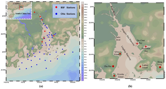
Figure 1.
(a) Spatial distribution of sampling sites in the study [36]. The red dots are BSF sites, and the blue dots are chlorophyll sites. They are evenly distributed in the Pearl River Estuary area; (b) Place names in the PRE region appearing in this article.
2.2. Data Sources
2.2.1. In Situ Data
Chlorophyll-a (Chla) data were collected in the field twice in 2016: once in the winter (February) and once in the summer (August). Figure 1 depicts the sites. The concentration of Chla (Cchla) was determined by spectrophotometry. Quantitative water samples were collected and filtered through 25mm Whatman glass fiber filters before being stored in a refrigerator. They were extracted in the laboratory with a 90% acetone solution and then measured with a spectrophotometer to determine Cchla [37].
In situ data on biodeposition fluxes were found in the literature. Only a few pieces of data on sedimentation fluxes were collected using sediment traps in China’s coastal waters. We applied the PRE annual average deposition flux data around 2000, which was acquired using the 210Pb-dating method [36]. Due to the age of the data, the geographic coordinates were appended based on labels of the sampling point map. The data needed to be converted to BSF before verifying accuracy.
2.2.2. Satellite Data
The remote sensing data used in this study include Landsat-5, Landsat-7, and Landsat-8 images. Images with less cloud cover and no missing cells are preferred. The selected images were mostly collected during the autumn and winter seasons. All Landsat images are downloaded from the United States Geological Survey (USGS) (https://glovis.usgs.gov/, accessed on 10 October 2021).
MODIS images and products corresponding to the time of the Landsat image were also used. MODIS images were used for spatiotemporal data fusion. Given the similarity of the water quality conditions in the PRE region, the differences in photosynthetically active radiation (PAR) values are minor. Due to the high temporal resolution of MODIS, the MODIS product corresponding to the time of each selected Landsat image can be obtained. Therefore, the PAR data were obtained by processing MODIS products.
Because no MODIS products were found before 2002, we needed to find their replacement. The bands of Sea-Viewing Wide Field-of-View Sensor (SeaWiFS) are the same as some bands of MODIS, and many ocean remote sensing retrieval algorithms are based on these two sensors [38]. In the study, the PAR products of SeaWiFS and MODIS data sources were obtained using the same algorithm with the same band of the two sensors. The error between using SeaWiFS products and MODIS products in this paper is small. Accordingly, we used SeaWiFS data as a supplement. MODIS images were downloaded from the National Aeronautics and Space Agency (NASA) data website (https://ladsweb.modaps.eosdis.nasa.gov/, accessed on 15 October 2021), and MODIS products were acquired from the Ocean Aqua data website (https://oceandata.sci.gsfc.nasa.gov/, accessed on 15 October 2021). SeaWiFS products were obtained from the Environmental Research Division’s Data Access Program (ERDDAP) website of the National Oceanic and Atmospheric Administration (NOAA) (https://oceanwatch.pifsc.noaa.gov/, accessed on 21 October 2021). Appendix A shows the specific data used in this paper.
2.2.3. Ancillary Data
The general bathymetric chart of the oceans (GEBCO) water depth data, with a spatial resolution of 15 arcs, were used in this study. This dataset was created using an algorithm and mathematical technology to interpolate measured water depth data. We downloaded them from GEBCO’s official website (https://www.gebco.net/data_and_products/histOrical_data_Sets/, accessed on 10 November 2021).
The POC deposition data were derived from the simulated distribution map [39]. Organic carbon sinks due to the complex power effect of gravity and salinity [40]. The POC deposition rate in the PRE was calculated using the well-validated one-dimensional river network and three-dimensional river hydrology and water quality model, in addition to the ROW-Column AESOP (RCA) water quality model. The simulation results could be used in further scientific research [39,41,42]. Temperature, salinity, diatom, blue algae concentrations and organic carbon concentrations of various solubility and granularity are among the parameters of the RCA three-dimensional water quality models. The one-dimensional river network was acquired based on the Saint-Venant equati which were solved using a three-level joint solution. The three-dimensional hydrodynamic model employed the Estuarine, Coastal and Ocean Modeling System with Sediments (ECOMSED). The inputted boundary conditions include water levels, tide, wind speed, wind direction and flow field.
The distributed graph was image digitized with matrix & laboratory (MATLAB) software. The POC sedimentation rate in each grid was extracted from the fake color display into the grid layer. After using ArcGIS software to georeference the layer, the 30 m resolution data were produced by bilinear interpolation. Its spatial resolution was consistent with the Landsat imagery. Appendix B shows the result.
2.3. Methods and Process
We preprocessed the downloaded Landsat image and then performed atmospheric correction. After that, in the SeaWiFS data analysis system (SeaDAS) software, the research area of MODIS PAR products was cut. Used the PAR data for bilinear interpolation to achieve the uniform spatial resolution as the Landsat image. To obtain sea surface temperature (SST), we applied the Google Earth Engine (Gee) platform. The Environment for Visualizing Images (ENVI) software was used to calculate water depth data, euphotic depth (Zeu), and chlorophyll-a concentration. Eventually, we used interface description language (IDL) and MATLAB software to write programs based on the chosen model and calculate the primary productivity and BSF in the PRE.
The accuracy of the BSF results was evaluated using the Pearson Correlation Analysis with Pearson’s correlation coefficient (R2) and significant value (P). We used the empirical orthogonal function analysis (EOF) method to analyze the spatiotemporal changes of BSF. The main water quality factors affecting BSF were determined using grey relational analysis (GRA). The corresponding pixel values of the two images are searched through a 7 × 7 window in GRA, with a comparison sequence established to calculate the grey relational grade (GRG). We assigned the window’s GRG value to the central pixel, and the window was cycled through to obtain the entire GRG distribution image [43,44]. Figure 2 shows the technical roadmap.
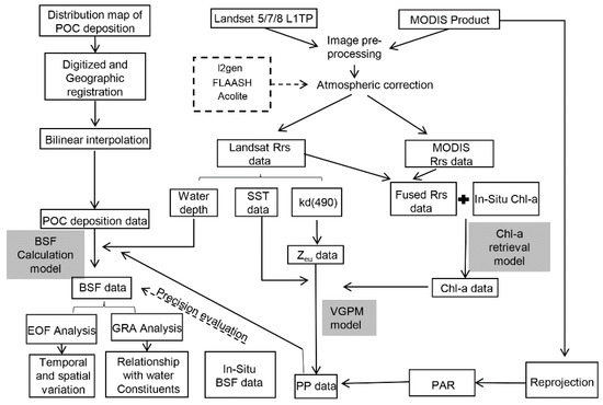
Figure 2.
The technical roadmap of this study. It illustrates key steps such as data sources, calculation procedures, and analysis methods. It also shows the model used in these steps.
2.4. Atmospheric Correction
In our study, the thematic mapper (TM) and enhanced thematic mapper (ETM+) images of Landsat5 and Landsat 7 were atmospherically corrected using the “Dark Spectrum Fitting” (DSF) algorithm in the Atmospheric Correction for OLI ‘lite’ (ACOLITE) software. To perform atmospheric corrections on MODIS images and Landsat-8 Operational Land Imager (OLI) images, we used the Management Unit of the North Seas Mathematical Models (MUMM) algorithm in the SeaDAS software.
2.5. Model Selection
2.5.1. Remote Sensing Spatiotemporal Fusion Model
The remote sensing spatiotemporal fusion model was used to select a better chlorophyll-a retrieval model. The enhanced spatial and temporal adaptive reflectance fusion model (ESTARFM) is currently the most widely used and mature; there are some improved methods based on it [45]. Our work applied the ESTARFM model. Appendix C depicts the model’s specific introduction and the effect of its use in this paper.
2.5.2. Chlorophyll-a Retrieval Model Based on Landsat Imagery
Chlorophyll-a retrieval was a step in calculating BSF. If Chla is calculated using remote sensing images with insufficient spatial resolution, the data within the PRE range can be covered by dozens of grids, which cannot adequately reflect the distribution. Therefore, the Chla retrieval algorithm should be established based on higher spatial resolution remote sensing images, such as Landsat.
In the absence of spectral data, the Chla data and remote sensing images must be consistent in time to construct a suitable chlorophyll-a retrieval model. However, the time of in situ data frequently deviates from the remote sensing images. Some studies generally used the method of averaging the measured data [46] or discarding some data. A higher resolution remote sensing image corresponding to the Chla data could be obtained after fusing the Landsat and MODIS images.
The Chla retrieval model used in this study is based on previous research findings and verified by ESTARFM and field data. Appendix D depicts the selected Chla retrieval model.
2.5.3. Sea Surface Temperature Retrieval Model
The SST in this work was retrieved with the Statistical Mono-Window (SMW) algorithm developed and used by Climate Monitoring Satellite Application Facility (CM-SAF). The algorithm is based on the linear radiative transfer equation for surface emissivity:
where Tb denotes the top-of-atmosphere brightness temperature in the Landsat’s thermal infrared channels, and ε is the surface emissivity. Ai, Bi and Ci are algorithm coefficients derived using the air temperature, water vapor, and ozone distribution datasets [47].
On the GEE platform, we calculated SST with the algorithm written by Ermida et al. [48].
2.5.4. Euphotic Depth Retrieval Model
The euphotic depth (Zeu) was typically calculated from the diffuse attenuation coefficient at 490 nm (Kd(490)). Ye [19] proposed the following relationship between Zeu and Kd(490) in the PRE region:
This equation was obtained by measuring the diffuse attenuation coefficients of the sites in the PRE area. Thus, this regional algorithm is more suitable for the field situation of the PRE compared with the general algorithm and the algorithm in other regions.
According to Yang’s research, the optimal Kd(490) retrieval model in PRE was determined with the collected field datasets [44]. This model was proposed by Tiwari et al. [49] in 2014:
where Rrs(670) refers to the reflectance of the water surface at 670 nm, which is the reflectance in the red band of Landsat images in this paper; Rrs(490) refers to the reflectance of the water surface at 490 nm, which is the reflectance in the blue band of Landsat images in this paper.
2.5.5. Empirical Method for Bathymetry
Liu [50] studied the Xisha Islands and provided a new empirical method to quickly estimate the water depths of optically shallow waters without in situ bathymetry data:
where mi denotes the coefficients estimated from known reflectance and water depth values, and q is a fixed constant that ensures a positive logarithm in all cases. The blue and green bands of the Landsat data were designated as band1 and band2, respectively.
Considering the GEBCO_2014 data as the known water depth value, the model with the highest correlation coefficient was obtained by fitting the reflectance after atmospheric correction (R2 = 0.64, q = 46, m1 = 2.142, m0 = 5.695). After the model retrieval, it was discovered that the estimated value in the PRE area does not correspond to the actual situation. The index retrieval model performs better due to the difference in water quality between the PRE and the Xisha Islands [51]. As a result, the water depth estimation model used in this paper is:
where band1 and band2 denote the blue and green bands of the Landsat data, respectively.
2.5.6. Primary Productivity Estimation Model
Few studies have investigated the primary productivity in the PRE with high spatial resolution satellite imagery. According to some researchers, the vertically generalized productivity model (VGPM) is the most applicable of all 24 models for estimating marine primary productivity, and the estimated value of primary productivity is relatively stable [52]. The parameters required by the VGPM model are chlorophyll concentration, sea surface temperature, photosynthetically active radiation and euphotic depth. Appendix E describes the VGPM model used in the paper.
2.5.7. BSF Estimation Model
Yang developed a method for estimating biosilica deposits using satellite remote sensing; the calculation equation is given [2]:
where Wopal denotes the BSF; PPnet is the marine primary productivity; LSRB is the POC deposition flux; D is the water depth and (Si:C) is the molar ratio of silicon to carbon in the water. Si:C ranges from 0.015 in oligotrophic central oceans to 0.45 in coastal waters [2]. In our study, we set the value to 0.3. This equation is obtained after correction in offshore waters using the relational equation between marine primary productivity and ocean bottom surface sediments proposed by Sarnthein et al. [53].
According to Yang’s discussion, this model is appropriate for calculating BSF in the estuary. Moreover, we overcome the limitations of this method to a certain extent. Yang considered only three main parameters, and the POC sinking flux was obtained based on an average estimate of the whole region. In our study, POC sedimentation data were calculated by inputting various parameters. As a result, we considered the effects of other variables, such as nutrients, water flow and algal concentration. The primary producers are primarily diatoms in the PRE [21,23]. Therefore, the sedimentation flux estimated from primary productivity is very close to the BSF. In conclusion, the model is suitable for this study.
3. Results
3.1. BSF Results
There are a lot of clouds in the PRE area for a long time, especially in spring and summer. As a result, very few Landsat images were available for remote sensing retrieval in the PRE each year. Therefore, the most suitable image, which has the least cloud cover over water in the PRE, is frequently acquired in autumn and winter. Figure 3 depicts the calculated BSF distribution of the PRE over 21 years. Clouds obscured the remote sensing images chosen in 2014, resulting in missing values in some areas.
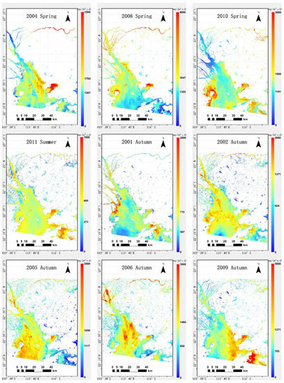
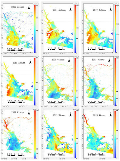
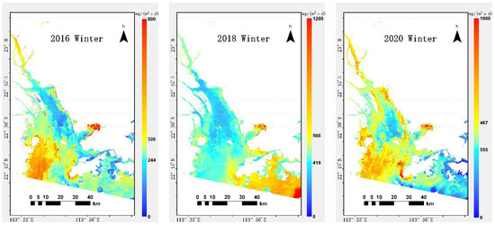
Figure 3.
The distribution results of BSF from 2000–2020 in the PRE. The distribution results are ordered by season. Due to the limitation of remote sensing data sources, only one image was selected for each year. There are three images in spring and only one result in summer. The unit of BSF is mg/(m2 × d).
The distribution results showed that the BSF is not a simple change trend along the coast to open water. There was no absolute difference in the magnitude of the BSF values on the west and east coasts, but the average values on coasts differed at various times. The changes in BSF values were spatially related to islands, waterways and bays, and shoals. Shenzhen Bay’s BSF value was 500–1000 mg/(m2 × d) higher than the surrounding waters almost every year. The BSF value of the Dragon’s Den Waterway (DDW) was usually lower than that of the surrounding waters. In autumn, the BSF value in the vicinity of the inlet shoal was significantly higher than in the surrounding waters. Except in winter, the BSF value around Qi’ao Island was generally higher than the surrounding waters.
The water quality conditions in the study area were generally consistent, so we averaged the BSF values across the study area for a time series analysis of annual changes. Because of the obvious difference in biogenic sediment between seasons, the analysis of changes in the mean value of the BSF should be divided into four seasons. However, there is only one distribution result in summer. Therefore, the BSF results in spring, autumn, and winter were chosen for mean comparison analysis, respectively. The results are shown in Figure 4.
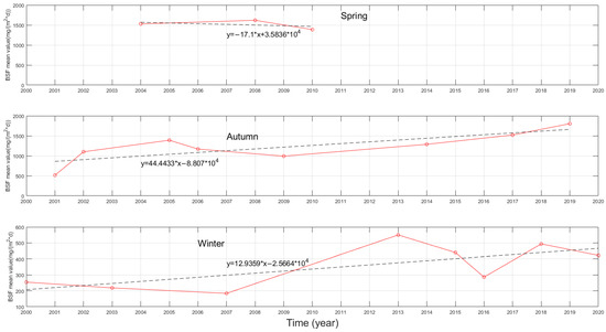
Figure 4.
The variation trend of the Pearl River Estuary’s average BSF value in spring, autumn, and winter from 2000 to 2020. Because there is only one distribution result in summer, no change trend analysis is performed. Based on the situation in winter and autumn, with more distribution results, the BSF has shown an overall increasing trend over the past 20 years.
In the springs of 2004, 2008, and 2010, the average value of BSF fluctuated around 1500 mg/(m2 × d), which shows a trend of first increasing and then decreasing. During the three-year spring period, the general trend slightly declined, and the slope of the trend line reaches 17 mg/(m2 × d) per year. Over the previous 21 years, the PRE’s average BSF value in autumn ranged from 500 to 2000 mg/(m2 × d), and it was between 100 and 600 mg/(m2 × d) in winter. Examining the change in BSF over the years, it generally showed an upward trend from 2000 to 2020, but fluctuated in some years. According to the growing trend, the BSF value in autumn is greater than that in winter, and the slope of the trend line reaches 44 mg/(m2 × d) per year. In the winter, it is only 12 mg/(m2 × d) per year. We also discovered the BSF in the PRE decreased from 2013 to 2016 in winter. This shows that the interannual variation of BSF in the PRE is increasing overall, but oscillating.
3.2. Accuracy Verification
Four calculated results were validated: chlorophyll-a, primary productivity, water depth and BSF. To some extent, Chla reflects the number of sedimentary organisms and is a key indicator for BSF calculation. The purpose of chlorophyll verification is to assess the uncertainty of the estimated value of the basic parameters in the BSF calculation process. The primary influencing factors of biological sedimentation in the biological sedimentation calculation model are primary productivity and water depth. As a result, the accuracy verification of the primary productivity and water depth results can determine the calculation process error. The accuracy verification of BSF is the final test of the feasibility of the method model in this paper. The accuracy verification was tested based on Pearson’s correlation coefficient (R2), significance value (p), slope, and root mean square error (RMSE). The fit effect will be better if the R2 and slope are closer to one, and the values of RMSE and p are lower.
3.2.1. Chla Results Verification
After excluding the interference of factors such as cloud cover and atmospheric correction failure, 32 pairs of satellite-retrieved data paired with observed stations were generated. Table 1 shows the three models that were compared with the single-band model used in this paper. The regionally tuned algorithm (RTA20) model was created for the Chla retrieval of the Landsat-8 satellite, which was applied to the Hong Kong coastal areas [54]. The symbolic regression (SR) model is a newly proposed Chla retrieval model suitable for the PRE region [55]. The sea surface multispectral index (SSMI) model is a model applied for Landsat-5 to retrieve offshore Chla [56]. Table 2 shows the fitted parameters between the in situ values and the retrieved values for the four models. Figure 5 depicts the relationship between field measurements and model retrieval results for the four algorithms, respectively.

Table 1.
The chlorophyll-a retrieval model used in this paper for accuracy comparison with the single-band model. B1, B2 and B3 represent blue band, green band and red band, respectively.
Table 2.
Statistical evaluation between the in situ Chla and the estimation value of Chla algorithms. The average in situ Chl-a value is 2.642 mg/m3.
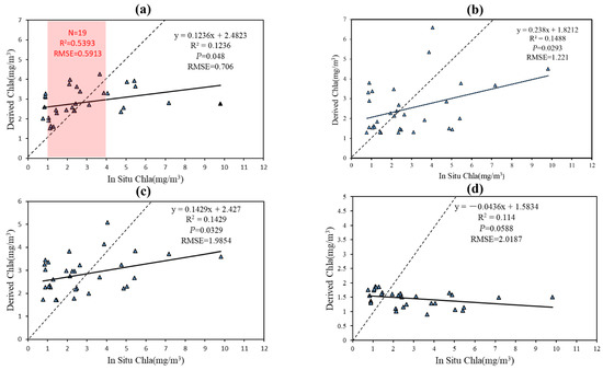
Figure 5.
Relationship between the value of in situ Chla and Chla estimated by the model (N = 32). The solid line is the fitted trend line, and the dashed line is the y = x line. (a) The single-band model used in this paper. The points in the red area are when the in situ Chla data is 1~4 mg/m3. The fitting effect is better, with the R2 reaching 0.5393; (b) The RTA20 model; (c) The SR model; (d) The SSMI model.
From Table 2, the R2, p, and slope show that the RTA20 model is more suitable. The RMSE shows that the single-band model is better than the other three models. The difference in R2 between single-band and RTA20 is 0.025, not notable. The difference in RMSE between the single-band model and RTA20 is 0.52, which shows that the stability of the RTA20 model is not as good as that of the single-band model. From Figure 5a, When the chlorophyll is in the 1~4 mg/m3 range, the R2 of the single-band model reaches 0.5393, and the RMSE of the single-band model is only 0.5913. Considering that the average value of Chla’s concentration in the PRE is 2.642 mg/m3, which is in the 1~4 mg/m3 range, the single-band model retrieves the Chla of most pixels more accurately due to the stability of the model and the distribution of Chla’s concentration in the PRE.
The possible reason that the model used in this paper suits BSF retrieval better than other models is the distribution of sampling points for the data used when building the model. Figure 1 shows that the sampling points used to build the model in this study are evenly distributed throughout the PRE. The sampling points used to build the RTA20 model are mainly distributed in the coastal waters of Hong Kong [54]. The sampling points used to build the SR model are arranged linearly from the PRE to the open sea [55]. The SSMI model is established based on the sampling point data of the Bangpakong River estuary [56]. Therefore, it is relatively better to use the single-band model with Landsat images to retrieve the Cchla of the whole PRE area in this study.
Overall, based on the above data and analysis, the single-band inversion model is better suited for retrieving the Chla using the Landsat satellite in this study.
3.2.2. Primary Productivity Results Verification
The PRE region was often covered by extensive cloud cover from April to September. Due to cloud interference and other factors, no field data corresponding to the time and space of Landsat remote sensing imagery were found for primary productivity. We looked for the previous literature on the primary productivity of the Pearl River Estuary [19,57,58] and compared the data to the primary productivity value of the corresponding period retrieved in this paper (Table 3). Because the study area of the paper is not exactly the same as the previous literature, the mean of primary productivity will differ.
Table 3.
Comparison of primary productivity averages retrieved in this article with other studies.
The primary productivity value calculated for each month in this study was compared with the primary productivity value calculated in the prior studies for the same season. We discovered that the differences were generally within 100 mg × m−2day−1 and that the change rule was basically the same. The researchers believe that the PRE’s primary productivity value is highest in September and lowest in February [19]. The primary productivity value in this study was also at its lowest in February. According to our findings, the primary productivity in the PRE increased significantly in March when compared with February. The results revealed a downward trend from March to June, implying that the average value for the entire spring was slightly lower than that of March, which is consistent with previous research findings.
3.2.3. Validation of Water Depth Results
We consider the average water depth values of different GEBCO versions to be real data. The 29 water depth values retrieved by the model were chosen at random by ArcGIS software. We used a polynomial inversion model [51] (Equations (7) and (8)) to compare with the water depth model used in this paper for accuracy verification. B1, B2, and B3 represent the blue band, green band, and near-infrared band, respectively. Table 4 shows the fitted parameters between the real values of water depth and the retrieved values for the two models. Figure 6 depicts the relationship between the real values and model retrieval results for the two algorithms, respectively.
Table 4.
Statistical evaluation between the in situ water depth and the estimation water depth value of the two algorithms.
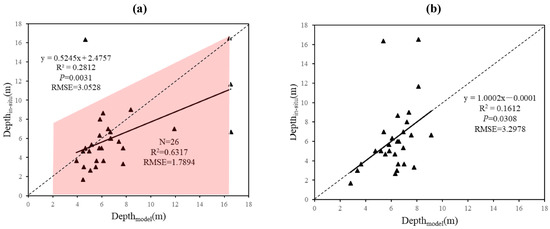
Figure 6.
Correlation between actual water depth and model retrieved water depth (N = 29). The solid line is the fitted trend line, and the dashed line is the y = x line. (a) The exponential model used in this paper. The points in the red area are when the retrieval water depth data is within 16.5 m, except an abnormal point. The fitting effect is better, with the R2 reaching 0.6317; (b) the polynomial model.
From Table 4, the R2, p, and RMSE show that the index model used in the paper is more suitable. The slope shows that the polynomial model is perfect. From Figure 6a, It is discovered that when the estimated water depth value is within 16.5 m, only two sample points deviate from the predicted line. After removing an abnormal point, it can be found that the R2 of the model used in the paper reaches 0.6317, and the RMSE of the model used in the paper is only 1.7894 when the estimated water depth value is within 16.5 m. At present, the applicable area for remote sensing water depth retrieval is a shallow water area, and the water depth in most areas of the PRE does not exceed 16.5 m [51,59]. From Figure 6b, although the slope of the trendline matches the y = x line very well, many points deviate from the trendline. As a result, the polynomial model is not stable enough in shallow water areas.
In general, based on the above data and analysis, the estimated water depth data meets the requirements of this work.
3.2.4. BSF Result Verification
The closest year to the BSF field measured data is 2000. Thus, we compared the satellite BSF retrieval results in 2000 with the BSF field data. The field data use the mean value calculated by the constant activity (CA) model and the constant flux of supply (CF) model [36]. To extract pixel values, we used the geographic coordinates of the place where the field data is located. The average proportion of biosilica in surface sediments is 1.42% [16]. The retrieved pixel values were converted to a sequence of BSF values, and the accuracy was checked between them and the measured value sequence. If there is no BSF value at the pixel point where the measured data is located, we referred to NASA’s Ocean Bioprocessing Group (OBPG) method for validating satellite data products using field measurements [60] as ground truth. A 3 × 3 pixel window is established centered on the measured data’s longitude and latitude; half of the pixels in the window are valid data, and the variance is less than 10%.
As shown in Figure 7, the R2 between the measured data and the model retrieval data is 0.8787. Additionally, the p is 0.0018 which shows a significant linear correlation between the two. The slope is 2.6666, which indicates there is a certain linear error between the retrieved value and the measured value, which may need to be converted to be equal. The RMSE (111.2374) shows that there is instability in the estimation method due to the small number of sample points. When the in situ value is in the 150–400 mg/(m−2day−1) range, three points are close to the fitted trend line (red zone), indicating that it is relatively reliable in this range. Because of the limitation of sampling at the observation sites, only a few data points are close to the 1:1 trend line. The reliability of the method is not sufficient to certify by relying on the fitting effect of the site data alone. Therefore, it is necessary to find other biodeposition data to assist in verification.
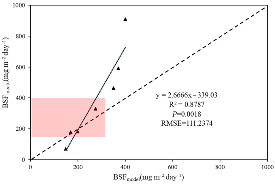
Figure 7.
Relationship between in situ BSF and BSF estimated by the model (N = 7). The solid line is the fitted trend line, and the dashed line is the y = x line. The three points in the red area are relatively close to the 1:1 trend line. It can be found that their in situ BSF values are between 150–400 mg/(m−2day−1).
To better demonstrate the accuracy of the BSF retrieval model in this paper, we collected biosilica data in the PRE for nearly two decades (Table 5). In general, the data of BSF are scarce. There is some information available on the biosilica content of sediments [61]. From Table 5, it is found that the BSF value estimated in the paper is in the same interval as that estimated in other literature. Three of the four sites showed greater BSF values estimated in this paper, while the biosilica content was higher in the other literature. In summary, under the premise of a certain error, the satellite inversion of BSF is proved feasible after the accuracy of the retrieval results is verified.
Table 5.
Comparison of data found in other literature with the retrieval results of the model in the paper. The units of some original data in other literature are inconsistent with this paper and have been converted.
3.3. Temporal and Spatial Variation of BSF
The EOF analysis was applied in this study to investigate the spatial patterns and temporal variability of BSF in different years. Since the number of BSF distribution maps in spring and summer were inadequate for EOF analysis, we performed EOF analysis separately for BSF in the PRE region during the autumn and winter periods. The first mode is chosen in both seasons; the mode chosen in autumn accounts for approximately 80.04% of the total variance, and the mode chosen in winter accounts for approximately 87.78% of the total variance.
Figure 8 depicts the principal components (PC) time series for the first EOF mode in both seasons. The PC values has both positive and negative values, indicating that the BSF fluctuates over time. The magnitude of the absolute value is related to the strength of the fluctuation. We observed that the PC values in the autumn of 2003 and 2013–2020 are negative, and the PC values in the autumn of the other years are positive. During the winter, PC values were positive for 2000–2010 and 2016, but negative for the other years.
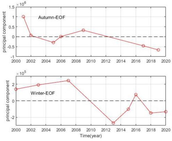
Figure 8.
The principal component (PC)’s time coefficients of the first EOF modes in the PRE waters during autumn and winter.
Figure 9 shows the spatial distribution of the first mode of EOF in autumn and winter, which accounts for more than 80% of the total variance. The eastern coast of the PRE has relatively high values in autumn, including the DDW, the eastern coast of Lantau Island and the coastal waters of Da Chan Bay, Shenzhen Bay, and Hong Kong. The areas with mangroves in Shenzhen Bay have large negative values. The waters from Qi’ao Island to Kyushu Island on the PRE’s west coast have lower values, while the shoals at the river entrance have higher values.
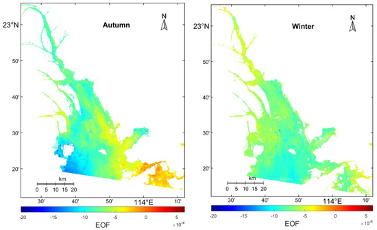
Figure 9.
The principal component (PC)’s spatial distribution of the first EOF modes in the PRE waters during autumn and winter.
In winter, the fluctuations in values were lower than in autumn, and the overall trend was the opposite of autumn. The PRE’s west coast had high-value regions. Values were also higher in the lower reaches of the Pearl River and its estuary, as well as in Hong Kong’s coastal waters. The value was generally low from the DDW to the outer sea via the Lingding Waterway.
3.4. Results of Water Constituents Affecting BSF
The optical properties of water are determined by the absorption or backscattering of different water constituents. This paper investigated the relationship between BSF and the two major water constituents. Figure 10 shows the distribution of spatial results obtained by calculating the GRG of the four seasons. In summer, only 2011 has high-quality remote sensing imagery, so we choose this. There are data from 2004, 2008, and 2010 available in spring. To better compare with the summer of 2011, the spring of 2010, which is closest in time to the summer of 2011, was chosen for analysis. In winter, the year 2000 was chosen because it is closest to the time of in situ verification data. In autumn, since the POC deposition data are based on 2006, the data in the autumn of 2006 were selected for calculating the GRG.
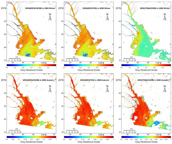
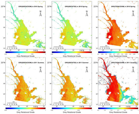
Figure 10.
The distribution of gray correlation between BSF and TSS or CDOM and between TSS and CDOM in the PRE region. The gray correlation grade between BSF and CDOM in the same season is roughly the same as that between BSF and TSS, but there are great differences in different seasons.
Total suspended solids (TSS) and chromophoric dissolved organic matter (CDOM) concentrations were retrieved concurrently with BSF using the same Landsat reflectance datasets. We calculated the TSS concentration with the TSS algorithm in the PRE developed by Guo et al. [62], and the CDOM concentration was calculated using the CDOM retrieval model proposed by Chen et al. [63,64]. The GRA was used to measure the relationship between BSF, CDOM and TSS for the four seasons, pixel by pixel (Figure 10).
In the PRE, GRGs between BSF and CDOM concentration (Ccdom) or TSS concentration (Ctss) are all higher on the west bank than on the east. The same holds for GRGs between Ccdom and Ctss. The magnitudes of the values of GRGs between BSF and either Ccdom or Ctss are not significantly different. Compared with GRGs between Ccdom and Ctss, GRGs between BSF and Ccdom or Ctss increased significantly in Shenzhen Bay and around Lantau Island. Seasonally, the GRG was higher in spring and summer than in autumn and winter between BSF and Ccdom or Ctss, with most pixels having values greater than 0.9. Equal situations were noticed in the GRGs between Ccdom and Ctss; although, the average value was lower than that between BSF and Ccdom or Ctss.
4. Discussion
4.1. Evaluation of BSF Results
Referring to the deposition process of organic matter in water proposed by Cai [4], Figure 11 shows the deposition pattern of the PRE. The biosiliceous sedimentation model demonstrates that biogenic sedimentation in water is extremely complicated, involving numerous physical, chemical and biological processes. The parameters used in the methodology for estimating BSF in the paper are the summary of these processes. For example, primary productivity in the calculation represents the primary producer in the pattern, which is the source of the BSF. In addition, the parameter of POC sedimentation rate reflects the sedimentation of biodeposition particles in the form of POC in water. Moreover, regardless of the flocculation process or the sedimentation of particles with the fluid, the water depth will affect the size of the sedimentation flux. As has been said, according to the deposition pattern in Figure 11, the BSF remote sensing retrieval method used in the paper has theoretical support.
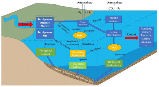
Figure 11.
The schematic diagram of estuarine deposition process. The BSF retrieval method used in the paper is theoretically supported by the complicated deposition patterns in the figure. The parts of primary productivity, POC and flocculating constituent are the main reflections of the calculation process. These parts also link remote sensing to the BSF.
From Table 6, we find that even though there is a certain error, at the same position, if the BSF value calculated by other papers is higher, the BSF estimated in this paper is also higher. Likewise, if the BSF values calculated in other literature are lower, the BSF values estimated in this paper are also lower. Therefore, spatially, the distribution prediction of BSF in this paper is relatively reliable. Meanwhile, more in situ data are required to improve the model’s accuracy. In brief, satellite remote sensing technology has the same application value as the current method of calculating BSF.
Table 6.
Comparison of the in situ BSF values of the station points in the literature with the BSF values estimated in this paper [36]. The BSF values of the stations are converted by the average proportion of biosilica in the sediments of the PRE.
The parameter calculation in the model is one aspect of errors in estimating BSF in this paper. There may be an error in retrieving the Chla, SST, and Zeu during the primary productivity calculation process. For example, the single-band model used in the Chla retrieval of the PRE is relatively stable, but it cannot accurately reflect micro-region anomalies. Since the SST was retrieved using the thermal infrared band, there was a tendency to overestimate in areas close to land. The POC deposition rate data used is simulated numerically, which may differ from the actual situation. Furthermore, calculating the 21-year BSF results with only the fall 2006 POC sedimentation rate would introduce an error. In addition, the accuracy of the water depth retrieval also needs to be improved.
We employed Landsat satellite images with a low temporal resolution. Using the imagery of a moment to calculate the BSF for the entire year will also result in errors. An error may happen when using the same retrieval algorithm on data from a different Landsat series of satellites. To solve the errors raised above, a unified conversion relationship can be established for the reflectance of the various images. Likewise, retrieval models of Chla and biological deposition can be developed for the TM, ETM+, and OLI images, respectively. It is possible that using spatiotemporal fusion methods to obtain monthly average images would reduce the errors in the following work.
Atmospheric correction is another step in the error source. The PRE region is classified as Case 2 waters, and precise atmospheric correction is a critical step in ocean color remote sensing [65]. Highly turbid coastal waters are more reflective, and TM/ETM+ images are better with the ACOLITE atmospheric correction algorithm [66]. The measured spectral data reveals that the atmospheric correction algorithm in the SeaDAS software is better suited for offshore OLI images [67,68,69]. In ocean color remote sensing, the Dark Spectral Fitting (DSF) atmospheric correction method is more appropriate for Landsat images than the Exponential Extrapolation (EXP) method [70]. Ye thought that the MUMM algorithm was the better atmospheric correction algorithm for high turbidity water at present [71]. Although employing the MUMM algorithm of SeaDAS and the DSF method of ACOLITE has certain errors, it is currently the better option.
Figure 12 shows the historical data on BSF changes according to the sampling of summer at a station in the PRE, which can roughly predict the BSF value of this station in the summer of 2011. Comparing the predicted value with the BSF values retrieved in this paper from Table 7, the ratio of uncertainty is about 35.99%. From the estimation model in this paper, the Si:C value for BSF calculation is 0.3, which is the average level of the ocean. The Si:C at the continental margin is generally smaller than 0.6 [61]. If the in situ BSF value is relatively large, the uncertainty error may be close to 50%. According to the accuracy verification results of Figure 7 in Section 3.2.4, in situ values were twice as high as estimated when the in situ BSF exceeded 600 mg/m−2day−1. This is most likely because the Si:C parameter is set too small. When the in situ BSF value is in 150–400 mg/m−2day−1 range, the error caused by Si:C is less noticeable. To reduce this error, it is necessary to use a mass of field data to obtain the optimum range of Si:C in the PRE.
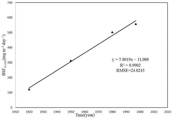
Figure 12.
The change trend of BSF at a station in the PRE over the past 100 years [29]. The sampling time is April of 1997. The value of BSF is obtained by conversion of deposition flux.
Table 7.
According to the historical data, the predicted value at the same sampling point is compared with the retrieved value in this paper. The unit of BSF is mg/(m−2day−1).
Additionally, because of the different optical properties of water bodies, more parameters may need to be considered to refine the calculation model. The particle size of sedimentary particles and the concentration of POC are the two key elements influencing the sedimentation process. Flow rate and nutrient concentration are two factors that affect the flocculation process. These parameters may be considered for introduction into the model in the next stage of work.
4.2. Relationship between BSF and Water Constituents
In addition to the parameters used in the BSF retrieval model, the water constituents include CDOM and TSS. Spectral absorption by CDOM is challenging for accurate Chla retrieval of turbid coastal waters [72]. TSS is crucial in the process of estuarine deposition [62]. The contribution of the two constituents varies across seasons for the same body of water. As a result, we explored the correlation between BSF and either Ccdom or Ctss in different seasons.
The GRA analysis results revealed that the BSF was closely related to TSS and CDOM. Figure 13 shows the subtraction of the two GRGs. Our results were credible according to Yang’s analysis method [44]. Displaying the subtracted positive values in red indicates that the GRGs of Ctss are higher than the GRGs of Ccdom, implying that the TSS plays a dominant role in the BSF. Negative values after subtraction are shown in blue, indicating that the GRGs of Ccdom are greater than the GRGs of Ctss, which means that CDOM plays a dominant role in BSF.
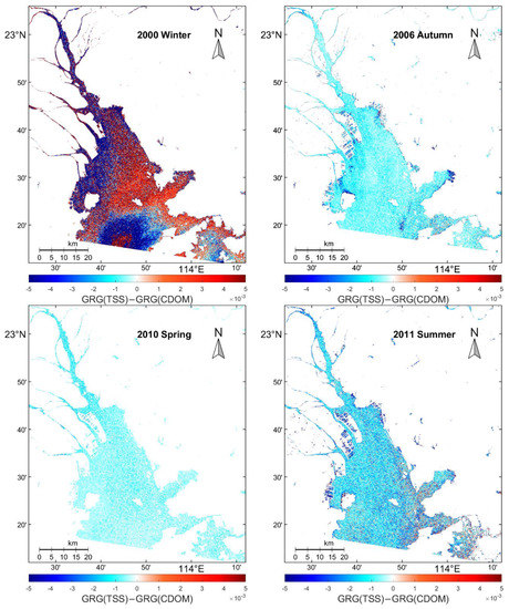
Figure 13.
Spatial distribution of the main water constituents affecting BSF in different seasons. The red area is larger than the blue in winter; the blue area is larger in autumn; in spring, the white area (the value is zero) is wider than in the other three seasons; and in summer, the red area is concentrated on the eastern coast of the PRE.
The effects of TSS and CDOM on BSF showed a certain seasonality. In winter, TSS has a greater impact on BSF in most PRE waters. This may be due to less precipitation in winter and generally higher Ctss in the PRE [73]. In autumn, CDOM mainly affects BSF. This may be attributed to the influence of the monsoon on the PRE in autumn. The downwelling caused by the northeasterly wind appears to reduce the amount of resuspension, causing the surface Ctss slightly decreasing [44]. In spring, the impact of the two is relatively balanced. During summer, the waters where TSS affects BSF are concentrated along the eastern coast. This condition appears to contradict the phenomenon of smaller Ctss in PRE’s southeastern region. We need to study the reasons for this result further. Ccdom correlates with the ebb and flow, and Ccdom has almost no seasonal variation [74]. Ctss and Ccdom are both influenced by tides, winds, circulation and river flow, but TSS may also be linked to climate change [62,72]. Therefore, seasonal variation in Ctss may be one of the reasons for seasonal variation in BSF, and previous studies have strongly supported the above findings.
Furthermore, upon analysis with Figure 10, it was discovered that in areas where the correlation between TSS and CDOM was low, the correlation between TSS and BSF was higher, particularly in summer and autumn. In above area, the Ccdom in the PRE region was greater in summer and autumn than in spring and winter, while the Ctss was the opposite. When the effect of Ccdom on the optical properties of water is much greater than that of Ctss, the intuitive expression is that the decrease of Ctss is more dramatic than the increase of Ccdom. At this point, the contribution of Ccdom to BSF has been saturated, and a small change in Ctss will cause a violent fluctuation in BSF.
4.3. Influence of Environmental Factors on BSF
The interannual variation trend of BSF is generally increasing with fluctuations in individual years, as the PRE region’s economic development and population grows. The spatial distribution of annual mean BSF and the EOF data can be employed to determine the temporal and spatial distribution rules of BSF. Further analysis of these rules reveals four major environmental factors influencing BSF.
4.3.1. Ecosystem
According to the BSF distribution from Figure 14 and EOF findings from Figure 9, the BSF values are often greater and more stable in Shenzhen Bay’s mangrove forests [75] and Tangjia Bay’s seagrass beds [76]. Some researchers revealed that different ecological environments, such as vegetation density, affect the deposition rate of biogenic sediment particles [77,78]. When there is a flow field in a mangrove ecosystem, mangrove roots enhance particle deposition. Meanwhile, they can prevent the resuspension of bottom sediment particles [78]. The more densely distributed mangroves there are, the more obvious this trend is [77]. Seagrass beds are not only highly productive ecosystems in coastal waters but also capture particulate matter [79]. Consequently, various ecosystems could influence BSF, such as mangroves and seagrass beds, which encourage biogenic sedimentation.
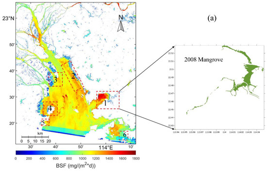
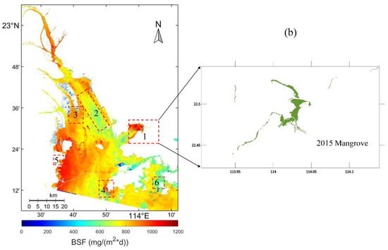
Figure 14.
Spatial distribution of annual mean BSF in the PRE region. (a) Using Landsat-5 as the original image inversion to get the average of BSF results, including the results of four seasons; (b) Using Landsat-8 as the original image inversion to get the average of BSF results, all in autumn and winter. Numbers represent different regions: (1) Mangrove area in Shenzhen Bay; (2) Flow field area of DDW; (3) Inlet shoal; (4) Waters around Qi’ao Island and Lantau Island; (5) Seagrass area in Tangjia Bay; (6) Upwelling waters to the southwest of Hong Kong. On the right are two mangrove distribution maps of Shenzhen Bay in representative years [75].
4.3.2. Flow Field
Figure 14 shows that the average BSF of the region where the flow field exists in DDW is different from the surrounding region. In spring and summer, the PRE is in a period of the rainy season, and nutrients from land sources enter the water body of the PRE along with the flow field [80]. As the water temperature gradually increases, nutrients cause the rapid reproduction and growth of phytoplankton, so the BSF of the flow field in spring and summer is relatively high. The growth of algae in the flow field in autumn and winter was inhibited by the disturbance of water flow [81]; therefore, the BSF value in the flow field was lower than that in the surrounding waters.
There is an upwelling in the southwestern waters of Hong Kong [82]; Figure 14 shows that there is a lower mean BSF relative to the surrounding waters. In the region with upwelling, the sedimentation rate is slowed down. Additionally, the resuspension phenomenon in the water body is exacerbated. This process may result in a decrease in the BSF value.
4.3.3. Islands and Reefs
Along the coasts of Qi’ao Island and Lantau Island, high BSF values are observed from Figure 14. When the flow field traverses islands and reefs, Von Karman vortices commonly form. The impact of eddying on nutrient distribution can increase the amount of small phytoplankton in the area [83]. This can explain why the nearby islands and reefs with flow fields have higher primary productivity. Therefore, the BSF value may rise in some coastal areas of Qi’ao Island and Lantau Island due to an increase in sedimentary organisms like diatoms.
4.3.4. Flocculation
It is observed from Figure 14 that the average BSF of the Inlet shoal is higher than that of the surrounding sea area. Additionally, this phenomenon is more noticeable in the flood season during summer and autumn than in the dry season during winter. These areas have higher algal productivity due to the Pearl River’s nutrient input, as well as being the confluence of fresh and brackish water. There are zones prone to flocculation because of variations in the salt content [84], and flocculation encourages biological deposition [4]. Furthermore, the sedimentation velocity of floc particle size in the PRE during the flood season is greater than that during the dry season [85], which is consistent with the retrieval BSF distribution in this paper in the estuarine and shallow watershed areas.
4.4. Prospect
There are two directions for future research on satellite retrieval of BSF. One is to enhance the retrieval model’s accuracy, taking into account the additional parameters, such as particle size and the gathering of more measured data to enhance the coefficient of determination’s accuracy. Moreover, it is possible to account for more precise information on POC settlement and water depth. The other is to improve the temporal and spatial resolution of the results. A daily BSF distribution map can be acquired using a multi-source spatiotemporal fusion model. Alternatively, we consider employing the Sentinel and GaoFen series with higher spatial resolution to assess the mechanism and process of biodeposition more precisely.
It is feasible to calculate the biosiliceous deposition in all estuaries around the world using the same remote sensing techniques as in the paper. The changing laws of biogenic sediment may differ for various types of estuaries.
5. Conclusions
In the paper, we used Landsat satellite imagery combined with MODIS products to estimate the BSF in the PRE. For the first time, the BSF distribution map in the PRE region during the past two decades was obtained, and the spatiotemporal characteristics and formation mechanism were explored based on this. We examined the interannual and seasonal variations of BSF in the PRE region, as well as the impact of TSS and CDOM on BSF. Ecosystems, islands and reefs, flow fields and flocculation are the four primary factors that influence biogenic sediment. Additionally, this study demonstrates that the multi-source remote sensing fusion model can be successfully applied to the estuary’s nearshore ocean color inversion.
Eventually, we discovered that retrieving biodeposition fluxes using high-resolution satellites like Landsat has application prospects. The results of this paper provide a possible remote sensing method for BSF monitoring in estuarine and coastal complex waters.
Author Contributions
Conceptualization, D.Y.; methodology, D.Y. and R.Z.; software, L.Z. and X.Y.; validation, R.Z.; formal analysis, R.Z.; data curation, L.Z.; writing—original draft preparation, R.Z.; writing—review and editing, D.Y. and R.Z.; supervision, D.Y.; project administration, D.Y.; funding acquisition, D.Y. All authors have read and agreed to the published version of the manuscript.
Funding
This research is jointly supported by the National Key R&D Program of China (grant no. 2022YFC3104901), and the Southern Marine Science and Engineering Guangdong Laboratory (Guangzhou) (grant no. GML2019ZD0602), and Hainan Province Science and Technology Plan Sanya Yazhou Bay Science and Technology City Science and Technology Innovation Joint Project (grant no. 2021CXLH0014).
Data Availability Statement
The data presented in this study are available on request from the corresponding author. GEBCO Compilation Group (2020) GEBCO 2020 Grid (doi:10.5285/a29c5465-b138-234d-e053-6c86abc040b9). GEBCO Compilation Group (2019) GEBCO 2019 Grid (doi:10.5285/836f016a-33be-6ddc-e053-6c86abc0788e). The GEBCO_2014 Grid, version 20150318, http://www.gebco.net, accessed on 10 November 2021.
Acknowledgments
The authors are very grateful to the USGS for providing the Landsat image data. The authors would like to thank NASA Goddard Space Flight Center and the NASA OBPG group for providing MODIS products and the SeaDAS software package. The authors would like to thank International Hydrographic Organization and Intergovernmental Oceanographic Commission for providing the GEBCO bathymetric data on the website. The authors are also appreciative of the researchers whose published literature contains the information used and cited in this paper, such as POC deposition rates.
Conflicts of Interest
The authors declare no conflict of interest.
Appendix A
Table A1.
The information of remote sensing data used in this paper.
Table A1.
The information of remote sensing data used in this paper.
| Year | Remote Sensing Image ID | Remote Sensing Product ID |
|---|---|---|
| 2000 | LE71220442000002SGS00 | sw_par_1d_2018_0_1baa_6f01_82fa |
| 2001 | LE71220442001260SGS00 | sw_par_1d_2018_0_111d_563f_d732 |
| 2002 | LE71220442002311EDC00 | aqua_par_1d_2018_0_928a_f116_5fc4 |
| 2003 | LE71220442003058SGS00 | A2003059052000.L2_LAC_OC |
| 2004 | LT51220442004069BJC00 | A2004069052500.L2_LAC_OC |
| 2005 | LT51220442005295BJC00 | A2005295052500.L2_LAC_OC |
| 2006 | LT51220442006314BJC00 | A2006314052500.L2_LAC_OC |
| 2007 | LT51220442007029BJC00 | A2007029052500.L2_LAC_OC |
| 2008 | LT51220442008064BKT00 | A2008064052500.L2_LAC_OC |
| 2009 | LT51220442009290BJC00 | A2009290053000.L2_LAC_OC |
| 2010 | LT51220442010085BKT00 | A2010085053000.L2_LAC_OC |
| 2011 | LT51220442011152BKT00 | A2011152052500.L2_LAC_OC |
| 2012 | LE71220442012307EDC00 | A2012308052000.L2_LAC_OC |
| 2013 | LC81220442013365LGN01 | A2013365052500.L2_LAC_OC |
| 2014 | LC81220442014320LGN01 | A2014320052500.L2_LAC_OC |
| 2015 | LC81220442015003LGN01 | A2015003052500.L2_LAC_OC |
| 2016 | LC81220442016038LGN01 LC81220442016086LGN01 LC81220452016038LGN01 LC81220452016086LGN01 MYD02HKM.A2016038.0525.061.2018055133234 MOD02HKM.A2016059.0235.061.2017325012149 MOD02HKM.A2016060.0320.061.2017325013357 MYD02HKM.A2016086.0530.061.2018057053639 MYD02HKM.A2016086.0525.061.2018057053740 | A2016038052500.L2_LAC_OC |
| 2017 | LC81220442017296LGN00 | A2017296052500.L2_LAC_OC |
| 2018 | LC81220442018043LGN00 | A2018043052500.L2_LAC_OC |
| 2019 | LC81220442019318LGN00 | A2019318052500.L2_LAC_OC |
| 2020 | LC81220442020337LGN00 | A2020337052500.L2_LAC_OC |
Appendix B

Figure A1.
The distribution map of POC sinking flux in the Pearl River Estuary.
Figure A1.
The distribution map of POC sinking flux in the Pearl River Estuary.

Appendix C
Remote sensing images must be preprocessed and resampled to the same size and resolution before using the ESTARFM algorithm. In the fusion process, the model uses the weight function to perform the convolution operation to obtain the central pixel value. First, the high-resolution and low-resolution images of the two phases are used to generate the high-resolution image of the predicted phase. The weighted combination of the two high-resolution prediction results produces a more accurate high-resolution image at the required moment [86].

Figure A2.
The flow diagram of the ESTARFM spatiotemporal fusion model.
Figure A2.
The flow diagram of the ESTARFM spatiotemporal fusion model.


Figure A3.
The true color images before space-time fusion and after space-time fusion. (a) The Modis image before using the ESTARFM model; (b) The fused image after using the ESTARFM model.
Figure A3.
The true color images before space-time fusion and after space-time fusion. (a) The Modis image before using the ESTARFM model; (b) The fused image after using the ESTARFM model.

The Landsat and MODIS images of the corresponding period of the measured chlorophyll were used in this paper, and the fusion result with the ESTARFM model is shown in Figure A3. The spatial resolution of the reflectance images obtained after fusion has significantly improved, which can be very useful for the selection and verification of chlorophyll inversion models. However, the reflectivity of the fused blue band differs significantly from that of the original MODIS image in some areas (the dark green area in Figure A3b), so pixels in this area should not be used when selecting models.
Appendix D
There are many algorithms for satellite retrieval of Chla, but few are applied to Landsat series satellites, especially in the turbid waters of the Pearl River Estuary. In order to select a suitable retrieval model, Pearson correlation analysis was performed on the reflectance of each band of the image obtained by fusion and the corresponding measured Chla data. This result is almost consistent with the results of the Pearson correlation analysis in previous studies (Figure A4). They analyzed the measured spectra equivalent to the Landsat spectral reflectance with the in situ Chla data [80,87]. Finally, the Landsat single-band spectral chlorophyll remote sensing retrieval model was selected. The model has not undergone multiple regressions and has good stability. The Chla inversion formulas for the four seasons from spring to winter are as follows:
where b2–b4 are the reflectance values of the second to fourth bands after Landsat image preprocessing, respectively. After spatiotemporal fusion, they can be regarded as the reflectance values of the three bands of visible light.
Chla = 81.33 × b4 + 0.00639
Chla = 18.039 × b3 + 0.28906
Chla = 102.7 × b3 + 0.10184
Chla = 20.71 × b2 + 0.495

Figure A4.
(a) Pearson’s correlation coefficient between measured spectra and in situ chlorophyll-a in the literature [80]; (b) Pearson’s correlation coefficient between the reflectance after spatiotemporal fusion and in situ chlorophyll-a in this study.
Figure A4.
(a) Pearson’s correlation coefficient between measured spectra and in situ chlorophyll-a in the literature [80]; (b) Pearson’s correlation coefficient between the reflectance after spatiotemporal fusion and in situ chlorophyll-a in this study.

Appendix E
In the VGPM model, the accuracy of different parameters in the Case2 waters will have a great impact on the estimated results [88]. Therefore, the model must be updated to account for different sea areas. This paper employed the simplified depth-integrated primary productivity calculation equation [19], which is as follows:
where PPeu is the primary productivity from the sea surface to the euphotic depth (mg C m−2 day−1); PBopt denotes the estimated maximum photosynthesis rate (mg C mg Chl-a−1 h−1); E0 is the daily PAR at the sea surface (mol quanta m−2); Zeu is the estimated euphotic depth; Copt is the chlorophyll-a concentration at the location of PBopt, replaced with the sea surface chlorophyll-a concentration; Dirr is the illumination time (h), and the Dirr in the PRE is 11.25 h.
In addition, the PBopt is pivotal for determining primary productivity. Recent research had shown that it is affected by both sea surface temperature (T) and chlorophyll-a concentration [89]. To control the errors caused by Chla in primary productivity results, PBopt was estimated using only sea surface temperature:
References
- Trujillo, A.P.; Thurman, H.V. Essentials of Oceanography, 11th ed.; Pearson Education: Hoboken, NJ, USA, 2014; pp. 98–99. [Google Scholar]
- Yang, D.; Yin, X. Potential deposition of biogenic silica source sediment in the Paleo-Yangtze Grand Underwater Delta estimated with satellite remote sensing. Mar. Georesour. Geotechnol. 2017, 36, 245–252. [Google Scholar] [CrossRef]
- Klyuvitkin, A.A.; Novigatsky, A.N.; Politova, N.V.; Koltovskaya, E.V. Studies of Sedimentary Matter Fluxes along a Long-Term Transoceanic Transect in the North Atlantic and Arctic Interaction Area. Oceanology 2019, 59, 411–421. [Google Scholar] [CrossRef]
- Cai, J.; Zeng, X.; Wei, H.; Song, M.; Wang, X.; Liu, Q. From water body to sediments: Exploring the depositional processes of organic matter and their implications. J. Palaeogeogr. 2019, 21, 49–66. [Google Scholar]
- Wang, X.; Zhang, H.; Han, G. Carbon Cycle and Blue Carbon Potential in China’s Coastal Zone. Bull. Chin. Acad. Sci. 2016, 31, 1218–1225. [Google Scholar]
- He, M.Q.; Cai, L.L.; Xu, J.; Li, X.F.; Shi, Z.; Jiao, N.A.Z.; Zhang, R. Sedimentation of psbA Gene-Containing Cyanophages, Cyanobacteria, and Eukaryotes in Marine and Estuarine Sediments. J. Geophys. Res. Biogeosci. 2021, 126, 14. [Google Scholar] [CrossRef]
- Talavera, L.; Vila-Concejo, A.; Webster, J.M.; Smith, C.; Duce, S.; Fellowes, T.E.; Salles, T.; Harris, D.; Hill, J.; Figueira, W.; et al. Morphodynamic Controls for Growth and Evolution of a Rubble Coral Island. Remote Sens. 2021, 13, 1582. [Google Scholar] [CrossRef]
- Dam, G.; Van der Wegen, M.; Taal, M.; Van der Spek, A. Contrasting behaviour of sand and mud in a long-term sediment budget of the Western Scheldt estuary. Sedimentology 2022, 69, 2267–2283. [Google Scholar] [CrossRef]
- Bale, A.J.; Uncles, R.J.; Villena-Lincoln, A.; Widdows, J. An assessment of the potential impact of dredging activity on the Tamar Estuary over the last century: Bathymetric and hydrodynamic changes. Hydrobiologia 2007, 588, 83–95. [Google Scholar] [CrossRef]
- Xia, M.; Zhang, C.; Ma, Z.; Liang, Z.; Zhou, X. 210Pb-dating method and determination of sedimentation velocity in Pearl River Estuary and Jinzhou Bay in the Bohai Sea. Scientia 1983, 5, 291–295. [Google Scholar]
- Nasiha, H.J.; Shanmugam, P. Estimation of settling velocity of sediment particles in estuarine and coastal waters. Estuar. Coast. Shelf Sci. 2018, 203, 59–71. [Google Scholar] [CrossRef]
- Nasiha, H.J.; Shanmugam, P.; Sundaravadivelu, R. Estimation of sediment settling velocity in estuarine and coastal waters using optical remote sensing data. Adv. Space Res. 2019, 63, 3473–3488. [Google Scholar] [CrossRef]
- Wang, Y.S.; Liang, X.L.; Flener, C.; Kukko, A.; Kaartinen, H.; Kurkela, M.; Vaaja, M.; Hyyppa, H.; Alho, P. 3D Modeling of Coarse Fluvial Sediments Based on Mobile Laser Scanning Data. Remote Sens. 2013, 5, 4571–4592. [Google Scholar] [CrossRef]
- Duan, D.D.; Ran, Y.; Cheng, H.F.; Chen, J.A.; Wan, G.J. Contamination trends of trace metals and coupling with algal productivity in sediment cores in Pearl River Delta, South China. Chemosphere 2014, 103, 35–43. [Google Scholar] [CrossRef] [PubMed]
- Zhang, L.; Yin, K.D.; Wang, L.; Chen, F.R.; Zhang, D.R.; Yang, Y.Q. The sources and accumulation rate of sedimentary organic matter in the Pearl River Estuary and adjacent coastal area, Southern China. Estuar. Coast. Shelf Sci. 2009, 85, 190–196. [Google Scholar] [CrossRef]
- Zhou, P.; Li, D.; Li, H.; Zhao, L.; Zhao, F.; Zheng, Y.; Wu, M.; Yu, H. Biogenic silica contents and its distribution in the sediments of the west Daya Bay. J. Appl. Oceanogr. 2019, 38, 109–117. [Google Scholar]
- Suess, E. Particulate organic-carbon flux in the oceans—Surface productivity and oxygen utilization. Nature 1980, 288, 260–263. [Google Scholar] [CrossRef]
- Armstrong, R.A.; Lee, C.; Hedges, J.I.; Honjo, S.; Wakeham, S.G. A new, mechanistic model for organic carbon fluxes in the ocean based on the quantitative association of POC with ballast minerals. Deep. Sea Res. Part II Top. Stud. Oceanogr. 2001, 49, 219–236. [Google Scholar] [CrossRef]
- Ye, H.B.; Chen, C.Q.; Sun, Z.H.; Tang, S.L.; Song, X.Y.; Yang, C.Y.; Tian, L.Q.; Liu, F.F. Estimation of the Primary Productivity in Pearl River Estuary Using MODIS Data. Estuaries Coasts 2015, 38, 506–518. [Google Scholar] [CrossRef]
- Zhang, Y.; Ghen, J.; Wang, J.; Han, Y.; Yi, L. Remote sensing inversion for net primary productivity and its spatial-temporal variability in Shenzhen coastal waters. J. Appl. Oceanogr. 2017, 36, 311–318. [Google Scholar]
- Dai, M.; Li, C.; Jia, X.; Zhang, H.; Chen, R. Ecological characteristics of phytoplankton in coastal area of Pearl River estuary. J. Appl. Ecol. 2004, 15, 1389–1394. [Google Scholar]
- Hu, X.Y.; Wang, Y.P. Coastline Fractal Dimension of Mainland, Island, and Estuaries Using Multi-temporal Landsat Remote Sensing Data from 1978 to 2018: A Case Study of the Pearl River Estuary Area. Remote Sens. 2020, 12, 2482. [Google Scholar] [CrossRef]
- Tang, S.; Cai, R.; Guo, H.; Wang, L. Response of phytoplankton in offshore China seas to climate change. J. Appl. Oceanogr. 2017, 36, 455–465. [Google Scholar]
- Chen, Y. Modern Sedimentary Velocity and Sedimentary Environment in the Pearl River Mouth. Acta Sci. Nat. Univ. Sunyatseni 1992, 31, 100. [Google Scholar]
- Chen, Y.; Luo, Z. Modern sedimentary velocity and their reflected sedimentary characteristics in the pearl river mouth. Trop. Oceanol. 1991, 10, 57. [Google Scholar]
- Liu, D.; Pan, D.L.; Bai, Y.; He, X.Q.; Wang, D.F.; Wei, J.A.; Zhang, L. Remote Sensing Observation of Particulate Organic Carbon in the Pearl River Estuary. Remote Sens. 2015, 7, 8683–8704. [Google Scholar] [CrossRef]
- Wang, Z.M.; Hu, S.B.; Li, Q.Q.; Liu, H.Z.; Liao, X.M.; Wu, G.F. A Four-Step Method for Estimating Suspended Particle Size Based on In Situ Comprehensive Observations in the Pearl River Estuary in China. Remote Sens. 2021, 13, 5172. [Google Scholar] [CrossRef]
- Yu, X.; Xu, J.; Long, A.; Zhong, W. Determination of suspended biogenic silica in the Pearl River Estuaryand its adjacent coastal waters in summer. J. Mar. Sci. 2018, 36, 67–75. [Google Scholar]
- Jia, G.; Peng, P.; Fu, J. Sedimentary records of accelerated eutrophication for the last 100 years at the pearl river estuary. Quat. Sci. 2002, 22, 158–165. [Google Scholar]
- Ye, H.B.; Chen, C.Q.; Yang, C.Y. Atmospheric Correction of Landsat-8/OLI Imagery in Turbid Estuarine Waters: A Case Study for the Pearl River Estuary. IEEE J. Sel. Top. Appl. Earth Observ. Remote Sens. 2017, 10, 252–261. [Google Scholar] [CrossRef]
- Nukapothula, S.; Chen, C.Q.; Wu, J. Long-term distribution patterns of remotely sensed water quality variables in Pearl River Delta, China. Estuar. Coast. Shelf Sci. 2019, 221, 90–103. [Google Scholar] [CrossRef]
- Wong, L.A.; Chen, J.; Xue, H.; Dong, L.X.; Su, J.L.; Heinke, G. A model study of the circulation in the Pearl River Estuary (PRE) and its adjacent coastal waters: 1. Simulations and comparison with observations. J. Geophys. Res. Ocean. 2003, 108, 17. [Google Scholar] [CrossRef]
- Hu, J.T.; Li, S.Y.; Geng, B.X. Modeling the mass flux budgets of water and suspended sediments for the river network and estuary in the Pearl River Delta, China. J. Mar. Syst. 2011, 88, 252–266. [Google Scholar] [CrossRef]
- Li, H.T.; Xie, X.T.; Yang, X.K.; Cao, B.W.; Xia, X.N. An Integrated Model of Summer and Winter for Chlorophyll-a Retrieval in the Pearl River Estuary Based on Hyperspectral Data. Remote Sens. 2022, 14, 2270. [Google Scholar] [CrossRef]
- Chen, C.Q.; Pan, Z.L.; Shi, P.; Zhan, H.G.; Larson, M.; Jonsson, L. Application of satellite data for integrated assessment of water quality in the Pearl River Estuary, China. In Proceedings of the 25th IEEE International Geoscience and Remote Sensing Symposium (IGARSS 2005), Seoul, Republic of Korea, 25–29 July 2005; pp. 2550–2553. [Google Scholar]
- Lin, R.; Min, Y.; Wei, K.; Zhang, G.; Yu, F.; Yu, Y. 210Pb-dating of sediment cores from the pearl river mouth and its environmental geochemistry implication. Geochimica 1998, 27, 401. [Google Scholar]
- Welschmeyer, N.A. Fluorometric analysis of chlorophyll-a in the presence of chlorophyll-b and pheopigments. Limnol. Oceanogr. 1994, 39, 1985–1992. [Google Scholar] [CrossRef]
- Shilin, T.; Chuqun, C.; Haigang, Z. Retrieval progress of ocean primary production by remote sensing. J. Oceanogr. Taiwan Strait 2006, 25, 591–598. [Google Scholar]
- Liu, G.; Hu, J.; Li, S.; Liang, B.; Huang, J. Simulation of organic carbon distribution and budgets during summer in the Pearl River Estuary. Acta Sci. Circumstantiae 2019, 39, 1123–1133. [Google Scholar]
- Wang, B.; Hu, J.T.; Li, S.Y.; Liu, D.H. A numerical analysis of biogeochemical controls with physical modulation on hypoxia during summer in the Pearl River estuary. Biogeosciences 2017, 14, 2979–2999. [Google Scholar] [CrossRef]
- Heng, Z.; Shi-yu, L.I. A numerical study on hypoxia and primary production in the Pearl River Estuary in summer using the modified RCA water quality model. J. Trop. Oceanogr. 2010, 29, 20–31. [Google Scholar]
- Liu, G.; Hu, J.; Li, S. Simulation of marine and terrestrial organic carbon in the Pearl River Estuary in summerdistribution characteristics, contribution rate and migration and transformation processes. China Environ. Sci. 2020, 40, 162–173. [Google Scholar]
- Wan, S.A.; Chang, S.H. Crop classification with WorldView-2 imagery using Support Vector Machine comparing texture analysis approaches and grey relational analysis in Jianan Plain, Taiwan. Int. J. Remote Sens. 2019, 40, 8076–8092. [Google Scholar] [CrossRef]
- Yang, C.Y.; Ye, H.B.; Tang, S.L. Seasonal Variability of Diffuse Attenuation Coefficient in the Pearl River Estuary from Long-Term Remote Sensing Imagery. Remote Sens. 2020, 12, 2269. [Google Scholar] [CrossRef]
- Liu, M.X.; Liu, X.N.; Dong, X.B.; Zhao, B.Y.; Zou, X.Y.; Wu, L.; Wei, H.J. An Improved Spatiotemporal Data Fusion Method Using Surface Heterogeneity Information Based on ESTARFM. Remote Sens. 2020, 12, 3673. [Google Scholar] [CrossRef]
- Liu, F.F.; Tang, S.L. Evaluation of Red-Peak Algorithms for Chlorophyll Measurement in the Pearl River Estuary. IEEE Trans. Geosci. Remote Sens. 2019, 57, 8928–8936. [Google Scholar] [CrossRef]
- Martins, J.P.A.; Trigo, I.F.; Bento, V.A.; da Camara, C. A Physically Constrained Calibration Database for Land Surface Temperature Using Infrared Retrieval Algorithms. Remote Sens. 2016, 8, 808. [Google Scholar] [CrossRef]
- Ermida, S.L.; Soares, P.; Mantas, V.; Gottsche, F.M.; Trigo, I.E. Google Earth Engine Open-Source Code for Land Surface Temperature Estimation from the Landsat Series. Remote Sens. 2020, 12, 1471. [Google Scholar] [CrossRef]
- Tiwari, S.P.; Shanmugam, P. A Robust Algorithm to Determine Diffuse Attenuation Coefficient of Downwelling Irradiance From Satellite Data in Coastal Oceanic Waters. IEEE J. Sel. Top. Appl. Earth Observ. Remote Sens. 2014, 7, 1616–1622. [Google Scholar] [CrossRef]
- Liu, Y.M.; Deng, R.R.; Qin, Y.; Cao, B.; Liang, Y.H.; Liu, Y.F.; Tian, J.L.; Wang, S.L. Rapid estimation of bathymetry from multispectral imagery without in situ bathymetry data. Appl. Opt. 2019, 58, 7538–7551. [Google Scholar] [CrossRef]
- Zhu, J.; Li, W.; Wang, G. Using remote sensing to define water depth in the pearl river estuary. Mar. Geol. Front. 2012, 28, 52–59. [Google Scholar]
- Carr, M.E.; Friedrichs, M.A.M.; Schmeltz, M.; Aita, M.N.; Antoine, D.; Arrigo, K.R.; Asanuma, I.; Aumont, O.; Barber, R.; Behrenfeld, M.; et al. A comparison of global estimates of marine primary production from ocean color. Deep. Sea Res. Part I Top. Stud. Oceanogr. 2006, 53, 741–770. [Google Scholar] [CrossRef]
- Sarnthein, M.; Winn, K.; Duplessy, J.C.; Fontugne, M.R. Global variations of surface ocean productivity in low and mid latitudes: Influence on CO2 reservoirs of the deep ocean and atmosphere during the last 21,000 years. Paleoceanography 1988, 3, 361–399. [Google Scholar] [CrossRef]
- Nazeer, M.; Bilal, M.; Nichol, J.E.; Wu, W.C.; Alsahli, M.M.M.; Shahzad, M.I.; Gayen, B.K. First Experiences with the Landsat-8 Aquatic Reflectance Product: Evaluation of the Regional and Ocean Color Algorithms in a Coastal Environment. Remote Sens. 2020, 12, 1938. [Google Scholar] [CrossRef]
- Huang, Y.Y.; Tang, S.L.; Wu, J. A chlorophyll-a retrieval algorithm for the Coastal Zone Imager (CZI) onboard the HY-1C satellite in the Pearl River Estuary, China. Int. J. Remote Sens. 2021, 42, 8365–8379. [Google Scholar] [CrossRef]
- Mahasandana, S.; Tripathi, N.K.; Honda, K. Sea surface multispectral index model for estimating chlorophyll a concentration of productive coastal waters in Thailand. Can. J. Remote Sens. 2009, 35, 287–296. [Google Scholar] [CrossRef]
- Cai, Y.; Ning, X.; Liu, Z. Studies on primary production and new production of the Zhujiang Estuary, China. Acta Oceanol. Sin. 2002, 24, 101–111. [Google Scholar]
- Yin, K.D.; Zhang, J.L.; Qian, P.Y.; Jian, W.J.; Huang, L.M.; Chen, J.F.; Wu, M.C.S. Effect of wind events on phytoplankton blooms in the Pearl River estuary during summer. Cont. Shelf Res. 2004, 24, 1909–1923. [Google Scholar] [CrossRef]
- Wang, Y.J. Application of Remote Sensing Technology to Map Water Depth by Weakening the Influence of Suspended Sediment. Doctor Dissertation, Nanjing Normal University, Nanjing, China, 2006. [Google Scholar]
- Bailey, S.W.; Werdell, P.J. A multi-sensor approach for the on-orbit validation of ocean color satellite data products. Remote Sens. Environ. 2006, 102, 12–23. [Google Scholar] [CrossRef]
- Qin, Y.C. Study on the Biogeochemistry of Sedimentary Silica in the Pearl River Estuary, China. Doctor Dissertation, Zhejiang University, Hangzhou, China, 2006. [Google Scholar]
- Guo, J.; Ma, C.L.; Ai, B.; Xu, X.P.; Huang, W.; Zhao, J. Assessing the Effects of the Hong Kong-Zhuhai-Macau Bridge on the Total Suspended Solids in the Pearl River Estuary Based on Landsat Time Series. J. Geophys. Res. Ocean. 2020, 125, 13. [Google Scholar] [CrossRef]
- Chen, J.; Zhu, W.N. Consistency evaluation of landsat-7 and landsat-8 for improved monitoring of colored dissolved organic matter in complex water. Geocarto Int. 2022, 37, 91–102. [Google Scholar] [CrossRef]
- Chen, J.; Zhu, W.N.; Pang, S.N.; Cheng, Q. Applicability evaluation of Landsat-8 for estimating low concentration colored dissolved organic matter in inland water. Geocarto Int. 2022, 37, 1–15. [Google Scholar] [CrossRef]
- Liu, H.Z.; Zhou, Q.M.; Wu, G.F.; Hu, S.B.; Li, Q.Q. Adaptation and validation of the swire algorithm for sentinel-3 over complex waters of pearl river estuary. In Proceedings of the 38th IEEE International Geoscience and Remote Sensing Symposium (IGARSS), Valencia, Spain, 22–27 July 2018; pp. 7933–7936. [Google Scholar]
- Xu, Y.; Feng, L.; Zhao, D.; Lu, J. Assessment of Landsat atmospheric correction methods for water color applications using global AERONET-OC data. Int. J. Appl. Earth Obs. Geoinf. 2020, 93, 102192. [Google Scholar] [CrossRef]
- Wei, J.; Lee, Z.; Garcia, R.; Zoffoli, L.; Armstrong, R.A.; Shang, Z.; Sheldon, P.; Chen, R.F. An assessment of Landsat-8 atmospheric correction schemes and remote sensing reflectance products in coral reefs and coastal turbid waters. Remote Sens. Environ. 2018, 215, 18–32. [Google Scholar] [CrossRef]
- Pahlevan, N.; Mangin, A.; Balasubramanian, S.V.; Smith, B.; Alikas, K.; Arai, K.; Barbosa, C.; Bélanger, S.; Binding, C.; Bresciani, M.; et al. ACIX-Aqua: A global assessment of atmospheric correction methods for Landsat-8 and Sentinel-2 over lakes, rivers, and coastal waters. Remote Sens. Environ. 2021, 258, 112366. [Google Scholar] [CrossRef]
- Ilori, C.; Pahlevan, N.; Knudby, A. Analyzing Performances of Different Atmospheric Correction Techniques for Landsat 8: Application for Coastal Remote Sensing. Remote Sens. 2019, 11, 469. [Google Scholar] [CrossRef]
- Vanhellemont, Q. Adaptation of the dark spectrum fitting atmospheric correction for aquatic applications of the Landsat and Sentinel-2 archives. Remote Sens. Environ. 2019, 225, 175–192. [Google Scholar] [CrossRef]
- Ye, H.B.; Yang, C.Y.; Tang, S.L.; Chen, C.Q. The phytoplankton variability in the Pearl River estuary based on VIIRS imagery. Cont. Shelf Res. 2020, 207, 104228. [Google Scholar] [CrossRef]
- Zhao, J.; Cao, W.X.; Xu, Z.T.; Ai, B.; Yang, Y.Z.; Jin, G.Z.; Wang, G.F.; Zhou, W.; Chen, Y.; Chen, H.Y.; et al. Estimating CDOM Concentration in Highly Turbid Estuarine Coastal Waters. J. Geophys. Res. Ocean. 2018, 123, 5856–5873. [Google Scholar] [CrossRef]
- Liu, R.Q.; Wang, Y.P.; Gao, J.H.; Wu, Z.Y.; Guan, W.B. Turbidity maximum formation and its seasonal variations in the Zhujiang (Pearl River) Estuary, southern China. Acta Oceanol. Sin. 2016, 35, 22–31. [Google Scholar] [CrossRef]
- He, Y.; Qin, Y.; Feng, Y.; Fu, Q.; Liu, C. Absorption characteristics of CDOM in the Pearl River Estuary at flood and ebb tides. Acta Sci. Nat. Univ. Sunyatseni 2018, 57, 22–31. [Google Scholar]
- Cheng, J.Y. Design and Production of Mangrove Remote Sensing Products and Data Sets in Guangdong-Hong Kong-Macao Greater Bay Area. Master Thesis, Jiangsu Ocean University, Lianyungang, China, 2022. [Google Scholar]
- Huang, X.P.; Jiang, Z.; Zhang, J.; Shi, Z.; Wang, F.; Ye, F.; Li, L. Newly discovered seagrass beds in the coastal seas of Guangdong Province. J. Trop. Oceanogr. 2010, 29, 132–135. [Google Scholar]
- Barcelona, A.; Serra, T.; Colomer, J. Fragmented Canopies Control the Regimes of Gravity Current Development. J. Geophys. Res. Ocean. 2018, 123, 1631–1646. [Google Scholar] [CrossRef]
- de Mendoza, F.P.; Fontolan, G.; Mancini, E.; Scanu, E.; Scanu, S.; Bonamano, S.; Marcelli, M. Sediment dynamics and resuspension processes in a shallow-water Posidonia oceanica meadow. Mar. Geol. 2018, 404, 174–186. [Google Scholar] [CrossRef]
- Liu, S.; Jiang, Z.; Wu, Y.; Zhang, J.; Zhao, C.; Huang, X. Mechanisms of sediment carbon sequestration in seagrass meadows and its responses to eutrophication. Chin. Sci. Bull. 2017, 62, 3309–3318. [Google Scholar] [CrossRef][Green Version]
- Luan, H. Based on Landsat8 the Suspended Sediment Concentration and Chlorophyll a Concentration of the Pearl River Estuary Remote Sensing Inversion and Time and Spatial Change. Master Thesis, Guangdong Ocean University, Zhanjiang, China, 2016. [Google Scholar]
- Sun, Y.; Luo, L.; Wei, G.; Zhai, H.; Li, F. Species Composition and Seasonal Variation in Phytoplankton at Dashahe Reservoir. Resour. Sci. 2014, 36, 1732–1738. [Google Scholar]
- Chen, X.R. Observation and Dynamical Analysis of Hydrographic Characteristics in the Pearl River Estuary in Summer of 2015. Master Thesis, Xiamen University, Xiamen, China, 2017. [Google Scholar]
- Liang, W.; Tang, D. Distribution characteristics of phytoplankton size structure in the western South China Sea in summer. J. Trop. Oceanogr. 2017, 36, 93–101. [Google Scholar]
- He, Y.; Gao, S.; Xu, F.; Hu, X. Key issues of the numerical model for tidal current and sediment transport in the Pearl River Estuary. J. Sediment Res. 2014, 4, 60–66. [Google Scholar]
- Deng, Z.; He, Q.; Yang, Q.; Lin, J. Observations of in situ flocs characteristic in the Modaomen Estuary of the Pearl River. Acta Oceanol. Sin. 2015, 37, 152–161. [Google Scholar]
- Zhu, X.L.; Chen, J.; Gao, F.; Chen, X.H.; Masek, J.G. An enhanced spatial and temporal adaptive reflectance fusion model for complex heterogeneous regions. Remote Sens. Environ. 2010, 114, 2610–2623. [Google Scholar] [CrossRef]
- Huang, Y.G. Remote Sensing Inversion of Water Quality Parameters in Internal Lingding of Pearl River Estuary Based on Field Spectral Data and Landsat8 OLI Image. Master Thesis, Guangzhou University, Guangzhou, China, 2017. [Google Scholar]
- Hyde, K.J.W.; O’Reilly, J.E.; Oviatt, C.A. Evaluation and application of satellite primary production models in Massachusetts Bay. Cont. Shelf Res. 2008, 28, 1340–1351. [Google Scholar] [CrossRef]
- Kameda, T.; Ishizaka, J. Size-fractionated primary production estimated by a two-phytoplankton community model applicable to ocean color remote sensing. J. Oceanogr. 2005, 61, 663–672. [Google Scholar] [CrossRef]


Disclaimer/Publisher’s Note: The statements, opinions and data contained in all publications are solely those of the individual author(s) and contributor(s) and not of MDPI and/or the editor(s). MDPI and/or the editor(s) disclaim responsibility for any injury to people or property resulting from any ideas, methods, instructions or products referred to in the content. |
© 2022 by the authors. Licensee MDPI, Basel, Switzerland. This article is an open access article distributed under the terms and conditions of the Creative Commons Attribution (CC BY) license (https://creativecommons.org/licenses/by/4.0/).