Article

The Influence of FY-4A High-Frequency LST Data on Data Assimilation in a Climate Model

1
Earth System Modeling and Prediction Centre, China Meteorological Administration, Beijing 100081, China
2
State Key Laboratory of Severe Weather, Beijing 100081, China
3
National Climate Center, China Meteorological Administration, Beijing 100081, China
4
Collaborative Innovation Center on Forecast and Evaluation of Meteorological Disasters, Nanjing University of Information Science and Technology, Nanjing 210044, China
5
Key Laboratory of Meteorological Disaster, Ministry of Education (KLME)/Joint International Research Laboratory of Climate and Environment Change (ILCEC)/Collaborative Innovation Center on Forecast and Evaluation of Meteorological Disasters (CIC-FEMD), Nanjing University of Information Science and Technology, Nanjing 210044, China
6
Anhui Climate Center, Hefei 230031, China
7
Institute of Atmospheric Physics, Chinese Academy of Sciences, Beijing 100029, China
8
Institute of Urban Meteorology, China Meteorological Administration, Beijing 100089, China
9
Hefei Meteorological Bureau, Hefei 230031, China
*
Author to whom correspondence should be addressed.
Remote Sens. 2023, 15(1), 59; https://doi.org/10.3390/rs15010059
Submission received: 10 November 2022 / Revised: 3 December 2022 / Accepted: 7 December 2022 / Published: 22 December 2022

Abstract

:
Based on the Beijing Climate Center’s land surface model BCC_AVIM2.0, an ensemble Kalman filter (EnKF) algorithm is developed to assimilate the land surface temperature (LST) product of the first satellite of Fengyun-4 series meteorological satellites of China to study the influence of LST data with different time frequencies on the surface temperature data assimilations. The MODIS daytime and nighttime LST products derived from Terra and Aqua satellites are used as independent validation data to test the assimilation results. The results show that diurnal variation information in the FY-4A LST data has significant effect on the assimilation results. When the time frequencies of the assimilated FY-4A LST data are sufficient, the assimilation scheme can effectively reduce the errors and the assimilation results reflect more reasonable spatial and temporal distributions. The assimilation experiments with a 3 h time frequency show less bias as well as RMSEs and higher temporal correlations than that of the model simulations at both daytime and nighttime periods. As the temporal frequency of assimilated LST observations decreases, the assimilation effects gradually deteriorate. When diurnal variation information is not considered at all in the assimilation, the assimilation with 24 h time frequency showed the largest errors and smallest time correlations in all experiments. The results demonstrate the potential of assimilating high-frequency FY-4A LST data to improve the performance of the BCC_AVIM2.0 land surface model. Furthermore, this study indicates that the diurnal variation information is a necessary factor needed to be considered when assimilating the FY-4A LST.

1. Introduction

The land surface temperature (LST) is a crucial land surface state variable for the energy budget at the surface which affects the distribution of sensible and latent heat flux and determines the upward thermal radiation from local to global scales [1,2]. As the ground-based observations are generally sparse over a wide geographic area, satellite remote sensing observation is the most effective way to measure LST at global and intercontinental scale [3]. The thermal infrared sensors and microwave sensors are two main satellite sensors for LST measurements. The passive microwave measurements can provide LST estimates for all weather conditions, but these products always have coarser temporal and spatial resolutions than infrared-based products. Although the infrared measurements are obscured by presence of clouds and can only provide LST for clear-sky conditions, they have smaller uncertainty than microwave-retrieved LST products. Therefore, the infrared-based LST data and products (e.g., the Moderate Resolution Imaging Spectroradiometer, MODIS) have been widely used in assessment of land surface trends, urban heat island detection, evaluation of land surface model, land data assimilation, land parameters retrieval, and several other global and regional applications [4,5,6,7,8,9,10,11,12] due to their high accuracy, sensor stability, and the convenient product availability. However, because MODIS sensors are carried on the polar-orbiting satellites, the diurnal LST observations at a given location are difficult to obtain. The diurnal variation of LST affected by the solar insolation, land cover characteristics, and atmospheric state [13] is also a key parameter and plays a vital role in surface energy balance and land-atmosphere interactions. Therefore, ignoring the daily variations will affect our understanding of the characteristics and changes of LST in global and regional scales.
Land surface data assimilation is an optimal technique that combines temporally discontinuous land observations with numerical models to obtain continuous land surface information in time and space on a large scale. In the last two decades, with the continuous enrichment of satellite LST products, many attempts have been made to assimilate LST from satellite observations at various temporal and spatial scales [4,14,15,16,17,18]. Huang et al. [19] developed a one-dimensional land data assimilation scheme based on an ensemble Kalman filter (EnKF) method to improve the estimation of the soil temperature profile. They demonstrated that the assimilation of MODIS LST is an effective way to improve the estimation of land surface state variables and fluxes. Ghent et al. [4] assimilated the daily MODIS LST using EnKF method and found an improvement in modeled LST and the reduction of uncertainty in modeling energy and water fluxes. Reichle et al. [20] performed the assimilation of satellite-derived skin temperature observations using an ensemble-based data assimilation method and found that the LST information was conducive to the improvement of land surface fluxes. Xu et al. [21] assimilated the FY3A-VIRR LST data using a dual-pass data assimilation scheme and found this new LST data from Chinese meteorology satellites reduced the uncertainties of land surface model and improved the prediction of surface energy fluxes. Chen et al. [22] developed a dual EnKF assimilation scheme to jointly assimilate Advanced Microwave Scanning Radiometer-Earth Observing System (AMSR-E) brightness temperature and MODIS LST products and demonstrated the potential of jointly assimilating land surface temperature to improve the estimation of soil moisture and related land surface model parameters. However, most of these LST assimilation studies were based on daily [23] or monthly scales [24] LST data and rarely considered the influence of LST diurnal variation in assimilation. Sgoff et al. [25] assimilated two-day synthetic LST data in a coupled land-atmosphere model and found the assimilation of hourly LST can reduce the error of the atmospheric boundary layer temperature forecast. Fu et al. [26] used a time resampling method to decompose the daily LST data of MODIS into 3 h intervals and found the diurnal variations of LST data can affect the sensitivity of assimilation. However, since these studies are mainly based on synthetic data or daily-scale MODIS data, the role of LST diurnal variation information in assimilation needs to be further verified with higher frequency real observation data. The high-frequency LST data from Geostationary Operational Environmental Satellite (GOES) has been assimilated to evaluate its impact on turbulent heat fluxes and surface heat fluxes [27,28], but few studies have been carried out on the effects of geostationary satellite LST assimilation on climate models.
The Fengyun-4 (FY-4) series meteorological satellites are the new generation of Chinese geostationary (GEO) orbit meteorological satellites of China [29]. The first satellite (FY-4A) was launched on 11 December 2016, which carried four optical instruments: the Advanced Geostationary Radiation Imager (AGRI); Geostationary Interferometric Infrared Sounder (GIIRS); Lightning Mapping Imager (LMI); and Solar X-EUV Imaging Telescope (SXEIT) [30]. Relying on these advanced instruments, the data and products of FY-4A have greatly enhanced capabilities for the applications in the monitoring and early warning of high-impact weather events [31,32], assimilations in numerical weather prediction (NWP), [33,34,35] and environment [36,37]. However, these assimilation studies of FY-4A data mainly focus on the NWP and nowcasting models with a short experimental period. The applications of FY-4A data and products in the field of climate are relatively weak compared to the weather field, especially in the application of quantitative assimilation in climate model. As a geostationary orbit satellite, an important advantage of the FY-4A satellite compared to a polar-orbiting satellite is that it can provide higher frequency LST observation products including diurnal variation information in the surrounding areas of China, which provides an important data source for us to explore the impact of hourly-scale LST data on climate models. However, there are still few studies exploring whether the climate models can benefit from the assimilation of high-frequency LST products from the FY-4A satellite.
The purpose of this paper is to explore the possible influence of the temporal frequency of LST observation on the performance of LST assimilation based on the land component model of the Beijing Climate Center Climate System Model (BCC_CSM). This study is organized into five sections. Section 2 introduces the observed data and verification data. The assimilation algorithm and experimental design are described in Section 3. The results of different temporal frequencies assimilation experiments are presented in Section 4. Finally, a summary and conclusions are given in Section 5.

2. Data

2.1. Forcing Data

The National Centers for Environmental Prediction (NCEP) atmospheric reanalysis data was used as the forcing data to drive the BCC_AVIM model in this study. The NCEP reanalysis data was based on 6-h forecasts of NCEP-NCAR reanalysis model with triangular 62 wave truncated horizontal resolution (approximately 2.5° × 2.5°). Four 6 h forecasts (0000, 0600, 1200, 1800 UTC) of seven essential variables (atmospheric pressure, precipitation rate, 2 m ground temperature, 10 m wind speed, relative humidity, downward shortwave radiation, and downward longwave radiation) were produced for each day. It was then interpolated to the BCC_AVIM spatial resolution of 1.125° × 1.125° grid using bilinear interpolation method. To meet the demand of BCC_AVIM, a smooth spline interpolation method is used to downscale the atmospheric forcing data to 3-h temporal resolution for the study.

2.2. Observation Data

The FY-4 satellite is the second generation of the Chinese geostationary meteorological satellite system, which provides higher quality and more refined temporal and spatial resolution than the first-generation geostationary orbital satellites from China [29,30]. The LST data of FY-4A satellite are produced from the brightness temperature of Advanced Geostationary Radiation Imager (AGRI) with 4 km spatial resolution and one hour temporal resolution. In order to be unified with the spatial resolution of the BCC model, the FY-4A data were interpolated from the original grid to the T106 gird (≈1.125° × 1.125°) of the BCC model using area weighted average spatial interpolation algorithm. The hourly FY-4A data are upscaled to 3 h resolution to ensure that there are enough observational sampling points at each assimilation time. Subsequently, the 3-h resolution data are further time-averaged to the 6-h, 12-h, and 24-h frequencies to obtain the observed data of assimilation experiments at different time frequencies.
In order to eliminate the outliers recorded in the FY-4A LST data that do not match the climate model, a quality control (QC) algorithm based on biweight coefficients was adopted before assimilation. The advantage of the biweight QC method [38] is that the statistical values are less affected by the outliers than the traditional QC methods. A brief description of the biweight QC algorithm is provided here. A weight function ( w i ) is computed as follows:
w i = X i M c × M A D
where X i is a sample of FY-4A LST observations, n is the number of samples, and M and MAD are the median and median absolute deviation, respectively. C is a parameter which all data beyond a certain critical distance from c are given zero weight. Then, the biweight mean and the biweight standard deviation (BSD) are calculated as:
X ¯ b i = M + i = 1 n X i M 1 w i 2 2 i = 1 n 1 w i 2 2
B S D = n i = 1 n X i M 1 w i 2 4 0.5 1 w i 2 1 5 w i 2
The X ¯ b i and BSD are then used to calculate the Z-score of the FY-4A LST data as:
Z i = X i X ¯ b i B S D
The Z-score values are used as the QC criterion for the FY-4A LST data. In Equations (2) and (3), the data close to the center of their distributions are given more weight than the tails. Thus, the X ¯ b i and BSD are more resistant to outlier values and can provide a more robust estimation of the mean and standard deviation of the samples of the FY-4A LST data than traditional statistical QC methods.

2.3. Verification Data

MODIS has seven surface temperature products [6]. The MOD11C1 and MYD11C1 LST products derived from Terra and Aqua satellites, respectively, are selected as verification data in this study. Both LST products contain LST variable and observation time information with 1 day temporal resolution and 0.05 spatial resolution. The temperature values in these two daily products are derived by reprojection and average of the values of MOD11B1, which produced by the day/night LST algorithm [39], at 6 km equal area grids in the sinusoidal projection. According to the constraints of solar zenith angle and the brightness temperature value by the day/night algorithm, each MOD11C1(MYD11C1) file contains daytime data and nighttime data as well as the observation time (UTC) data for the temperature value at each grid. The quality control (QC) flag in MOD11C1 and MYD11C1 provide identification information on the quality of the product at each grid. Because the LST data from MODIS are often contaminated by clouds, only the LST observations with a “00” QC flag (average LST error ≤ 1 K) are selected as verification data for the assimilation experiments. With the observation time information of each grid, it can be easily obtained every grid with valid LST value of the MODIS data fall in which 3-h time interval. Therefore, the LST data from MOD11C1 and MYD11C1 are reprocessed at the 3-h frequency to unify with the time resolution of the FY-4A observation and the BCC_AVIM2.0 model output. In this study, both the daytime data and the nighttime data mainly include two 3-h time intervals (00-03 and 03-06 UTC for daytime data, while 12–15 and 15–18 UTC for nighttime data). It was interpolated on a grid of T106 using area weighted average spatial interpolation method.

3. Model, Assimilation Algorithm, and Experimental Design

3.1. Land Surface Model

The BCC_CSM2_MR model is a fully coupled global climate system model including the atmospheric, land, ocean and sea ice components models [40]. These components of the model interact with one another at their interfaces through water flux, energy flux, and momentum flux. The land component model in the BCC-CSM2-MR is the BCC Atmosphere and Vegetation Interaction Model Version 2 (BCC_AVIM2.0). It originates from the NCAR Community Land Model version 3.0 (CLM3) [41] and the Atmosphere and Vegetation Interaction Model (AVIM) [42,43] with major framework to include physiological, biophysical, and soil carbon–nitrogen dynamical processes. It has made improvements in the scheme of snow surface albedo and snow cover fraction, a variable temperature threshold to determine soil water freezing–thawing, a dynamic phenology for deciduous plant function types, and a four-stream approximation of solar radiation transfer through vegetation canopy [44].
In the BCC_AVIM2.0, the LST at the n + 1 time step are calculated as:
T g n + 1 = S g L g H g λ E g + T g n L g T g H g T g + λ E g T g L g T g H g T g + λ E g T g
where S g is the solar radiation absorbed by the ground ; L g is the longwave radiation absorbed by the ground (positive toward the atmosphere); H g is the sensible heat flux from the ground; and λ E g is the latent heat flux from the ground.
The partial derivative of the net longwave radiation, the sensible flux, and the latent heat flux are calculated as:
L g T g = 4 ε g σ T g n 3
H g T g = ρ atm C p γ ah
E g T g = ρ atm γ aw dq g dT g
where σ is the Stefan-Boltzmann constant; ε g is the ground emissivity; ρ atm is the density of atmospheric air; C p is the specific heat capacity of air; γ ah is the aerodynamic resistance to sensible heat transfer; γ aw is the aerodynamic resistance to water vapor transfer; and q g is the specific humidity of the soil surface.

3.2. Assimilation Algorithm

The EnKF method [45] is a Monte Carlo approximation to the traditional Kalman filter [46]. It provides a flow-dependent background error covariance at each update step by propagating an ensemble of state vectors and corrects the background optimally to newly available observations. Assuming mean-zero Gaussian random error q t 1 i with covariance Q t 1 added to the state variable, when no FY-4A LST observation exists, the evolution of each ensemble member of state variable x i can be expressed as:
x t i = f t x t 1 i + + q t 1 i ,   q t 1 i ~ N 0 , Q t 1
The superscript “i” indicates the ensemble members. The superscripts “–” and “+” refer to state variables in the forecast step and update step, respectively. The nonlinear operator f · denotes the land surface model processes containing state variables x i .
When LST observations are available, each ensemble member of state variable is updated using the following equation:
x t i + = x t i + K t   y t i H t x t i
K t = P t H t T   H t P t H t T + R t 1
where H t is the measurement operator, and y t i is the i-th ensemble member of the observation ensemble generated by perturbing the actual observation with mean-zero random error η t i [47]. K t is the Kalman gain matrix. P t and R t are the forecasted background error covariance matrix and observation error covariance matrix, respectively. P t is calculated as the sample covariance from ensemble of model state variables:
P t = 1 n 1 X t X t T
where X t = x t 1 x ¯ t , x t n x ¯ t , and x ¯ t = 1 n i = 1 n x t i is the mean value of forecasted state variables at the time t.
The assimilation strategy of FY-4A LST data is illustrated in Figure 1. The BCC_AVIM2.0 model was driven by atmospheric forcing fields to retrieve the background field of LST. When the FY-4A LST existed, the LST background ensemble and observation ensemble were obtained by adding random disturbances to the background field and observation field, respectively. Then the EnKF algorithm was used to update the LST analysis ensemble samples, and the LST analysis field was obtained by the averaged value of the ensemble members. When the FY-4A LST did not exist, no assimilation update was performed, and the LST analysis field was directly replaced by the LST background field at this time step. Then, the LST analysis field was integrated forward as the background field for the next time step. This process looped continuously throughout the assimilation experiment period.

3.3. Experimental Design

The assimilation experiments of this study were conducted during a two-year period from 1 January 2017 to 31 December 2018. The first year of this experiment period (from 1 January 2017 to 31 December 2017) was looped three times to spin up the BCC_AVIM2.0 for obtaining reasonable and stable initial-state variables of the model. The ensemble size is set to 100 for the assimilation experiments. The time step of the BCC_AVIM2.0 is half an hour.
In order to explore the effect of LST observation frequency on the assimilation performance, four assimilation experiments with different time frequencies (abbreviated as ASS 3 h, ASS 6 h, ASS 12 h, ASS 24 h) of hourly FY-4A LST observations were assimilated, and one model control experiment (CTL) was conducted in this study. The difference between these assimilation experiments is the temporal frequency of the input LST observations. The FY-4A data for each time frequency are the average value of the LST in this time period. The high-frequency observations (e.g., 3 h) can provide more diurnal variation information of LST than low-frequency data (e.g., 24 h). Taking the ASS 3 h experiment as an example, at each time step during the 3 h period, the FY-4A observations of this 3 h period were assimilated to update the statements of the grids with observation data. Grids without observations were not updated.
Because MODIS LST products have observation time information at each grid point, the MODIS verification data in this study are reprocessed to the same temporal (3 h) resolution as the outputs of model. For each 3 h period, the MODIS LST data are retained only for grid points with the observation time exactly within this 3 h period. Since the simulation and assimilation output data have global coverage at all temporal frequencies, in order to maintain consistency with the MODIS validation data, only the grid points where the MODIS data have values in the CTL and ASS experiments were selected for result analyses.
Since the FY-4A LST data mainly cover China and surrounding areas, the assimilation experiment region is selected as 70°E–150°E and 10°N–60°N. The performances of different experiments were evaluated quantitatively based on several common statistical indices, including the bias, root-mean-square error (RMSE), and correlation coefficient (CC). The bias was used to evaluate the average systemic bias to the MODIS data between CTL and different ASS experiments; the RMSE was used to determine the total magnitude of the difference, and the CC was used to reflect the linear consistency of the temporal variability. The values of bias, RMSE and CC, are calculated as follows:
  BIAS = 1 n 1 n X i X i o
  RMSE = 1 n 1 n X i X i o 2
CC = 1 n X i X ¯ X i o X ¯ i o 1 n X i X ¯ 2 · 1 n X i o X ¯ i o 2
where n is the number of 3 h periods during the entire study period; X i and X i o are the simulation/assimilation experiment outputs and the MODIS verification data at time i, respectively; and X ¯ i o and X ¯ i o are the time-averaged values of X i and X i o , respectively.

4. Results and Analysis

4.1. Spatial Distribution of Annual-Mean LST

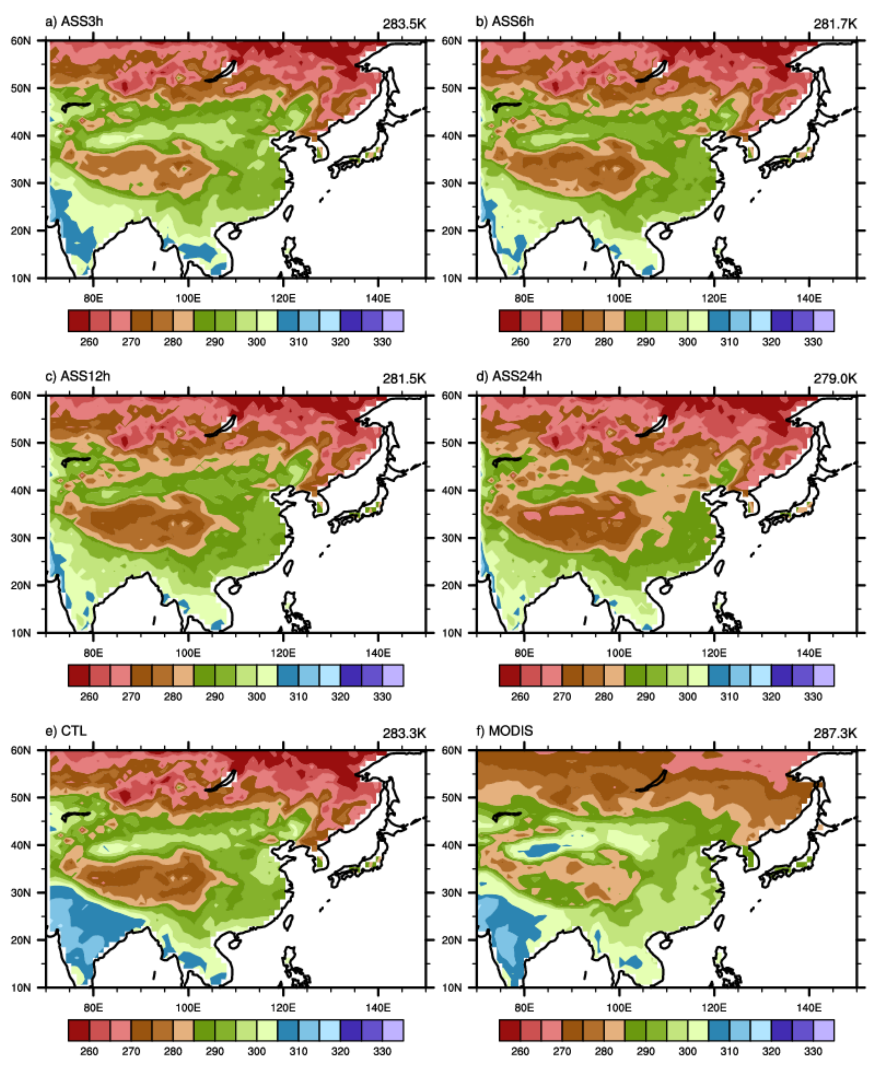
The spatial distribution of LST is one of the important indicators of the basic characteristics of LST. The spatial distributions of the annual mean of LST over the study period from MODIS daytime LST data and the CTL run experiment before assimilation as well as assimilation experiments with different time frequencies for the corresponding period are shown in Figure 2. The spatial distribution of MODIS daytime LST over China shows a southwest-to-northeast sandwich distribution in annual mean (Figure 2f). The highest annual mean LST is observed over the Indian peninsula. Then the LST decreases with increasing latitude and reaches a relatively low-value area over the Tibet Plateau. The LST increases northward to Xinjiang and Inner Mongolia with latitude and then decreases with latitude toward the north. The spatial distributions of the CTL experiment and all assimilation experiments are generally consistent with the MODIS observations over the study area. The regional-mean LST of the CTL simulation was 4 K lower than that of the MODIS data. The LST of the CTL simulation is higher than MODIS in the Indian peninsula but lower in the Tibet Plateau, and the range and intensity of the low LST area near high latitudes are larger than those observed by MODIS (Figure 2e). The assimilation experiments with different frequencies showed different assimilation results. Among all the assimilation experiments, the ASS 3 h experiment took into account the influence of the diurnal variation of the FY-4A LST data most comprehensively, which improved the LST statement compared with the CTL experiment (Figure 2a). The assimilation did not improve the overall LST results when reducing the temporal frequency of the FY-4A LST observations. The regional-mean values of LST of ASS 6 h, ASS 12 h, and ASS 24 h experiments were lower than that of the CTL experiments. The bias in the assimilation results gradually increases as the temporal frequency of the assimilated data decreases (Figure 2b–d). When the diurnal variation of LST was not considered in the assimilation, it produced a significant negative bias (about −8 K) compared with the MODIS LST data over the whole study area (Figure 2d). This may be due to the fact that the LST itself has strong diurnal variation information. If the diurnal variation characteristics of LST are ignored during the assimilation experiment, additional bias will be introduced during the assimilation process, thus affecting the overall assimilation effect of the assimilation experiment.
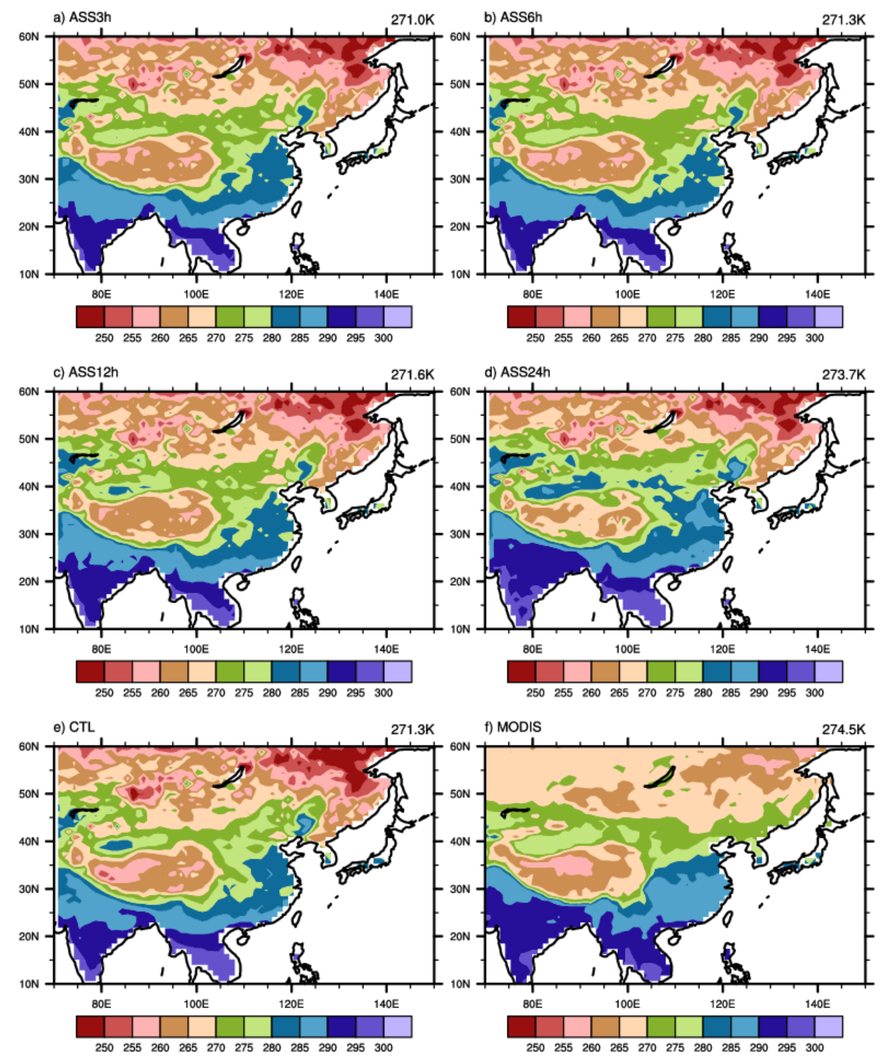
Figure 3 shows the spatial distributions of the annual mean of LST over the study period for the MODIS nighttime data, the CTL, and different frequencies assimilation experiments. Compared with the daytime results, the LST of nighttime for all experiments are significantly lower. For the results of MODIS data, it is about 13 K lower than the daytime data for the regional-mean LST value (Figure 3f). The differences between different assimilation experiments (Figure 3a–d) are within 2.7 K and are smaller than that of the daytime results which are about 4.5 K. It can also be seen that as the temporal frequency of the assimilated LST gradually decreases, the assimilated regional-mean LST values gradually increases. The regional-mean LST for the ASS 24 h experiment is 2.7 K higher than the ASS 3 h experiment. Combined with the daytime results, it can be found that when the time frequency of the FY-4A observation becomes smaller, the assimilation results gradually tend to the daily-mean values of LST. Since the nighttime LST results of the CTL experiment and all assimilation experiments are smaller than that of MODIS data, the regional-mean LST value of the ASS 24 h experiment (Figure 3d) is superimposed with a positive bias compared with that of the ASS 3 h experiment, resulting in the results of the ASS 24 h experiment being the closest to the MODIS verification data in all the nighttime assimilation experiments.

4.2. Spatial Distribution of Bias

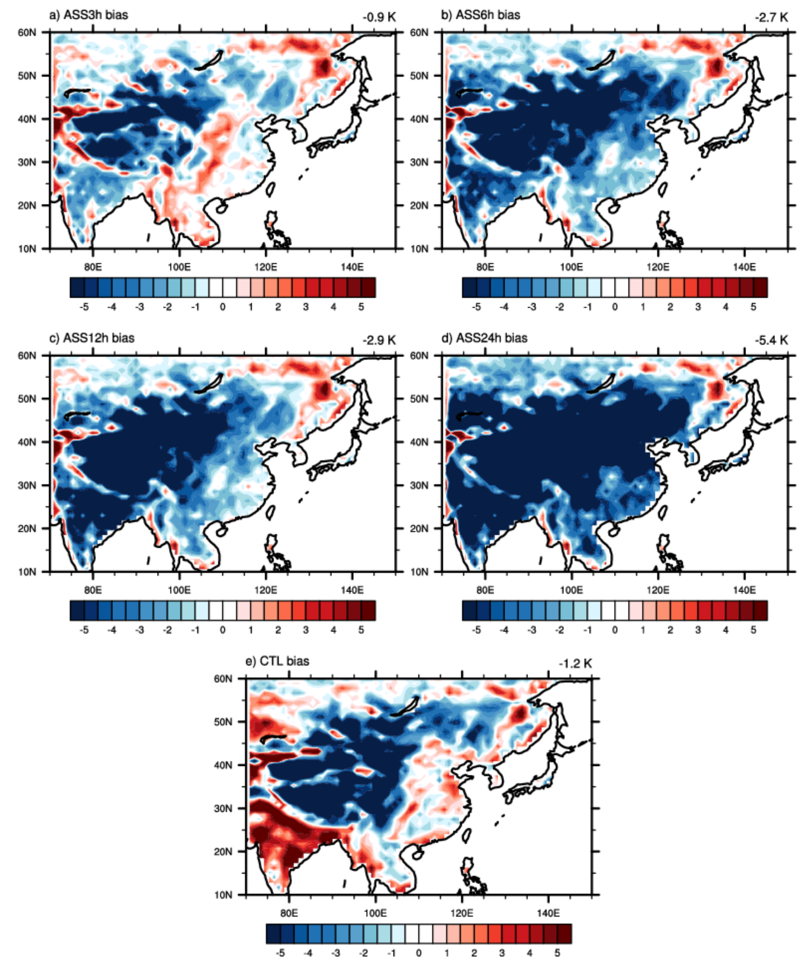
Figure 4 shows the spatial distributions of the daily-mean bias of the CTL experiment and assimilation experiments versus the daytime MODIS data. The CTL experiment significantly underestimates the LST over western China and overestimates it over the Indian peninsula (Figure 4e). The bias can reach more than −5 K over western China and Mongolia and more than 4 K over the Indian peninsula. Western China is dominated by plateau areas with an average altitude of more than 1000 m. The obvious negative bias over western China and Mongolia may be mainly due to the overestimation of the surface albedo in the plateau area of the BCC_AVIM2.0 model [44]. The biases of the ASS 3 h experiment are better than that of the CTL experiment (Figure 4a), while the biases of other assimilation experiments with observation data frequencies of 6 h and longer are worse than that of the CTL experiment (Figure 4b–d). In the assimilation of daytime LST data, it is possible that the LST can change significantly in a short time due to the large variability during the daytime. Therefore, when the time frequency of the FY-4A LST data is less than 6 h, there will be large bias in the assimilation process due to insufficient time representativeness of the LST observation data, which can worsen the assimilation results and lead to a larger bias after assimilation than in the CTL experiment. For example, the regional-mean bias of the ASS 24 h experiment is almost doubled compared to that of the ASS 12 h experiment. It indicates that if it only assimilates the daily-scale FY-4A LST data, the large negative biases of the daily-scale FY-4A LST data compared with to daytime FY-4A LST data cause the significant biases of the ASS 24 h experiment compared to the MODIS daytime verification data.
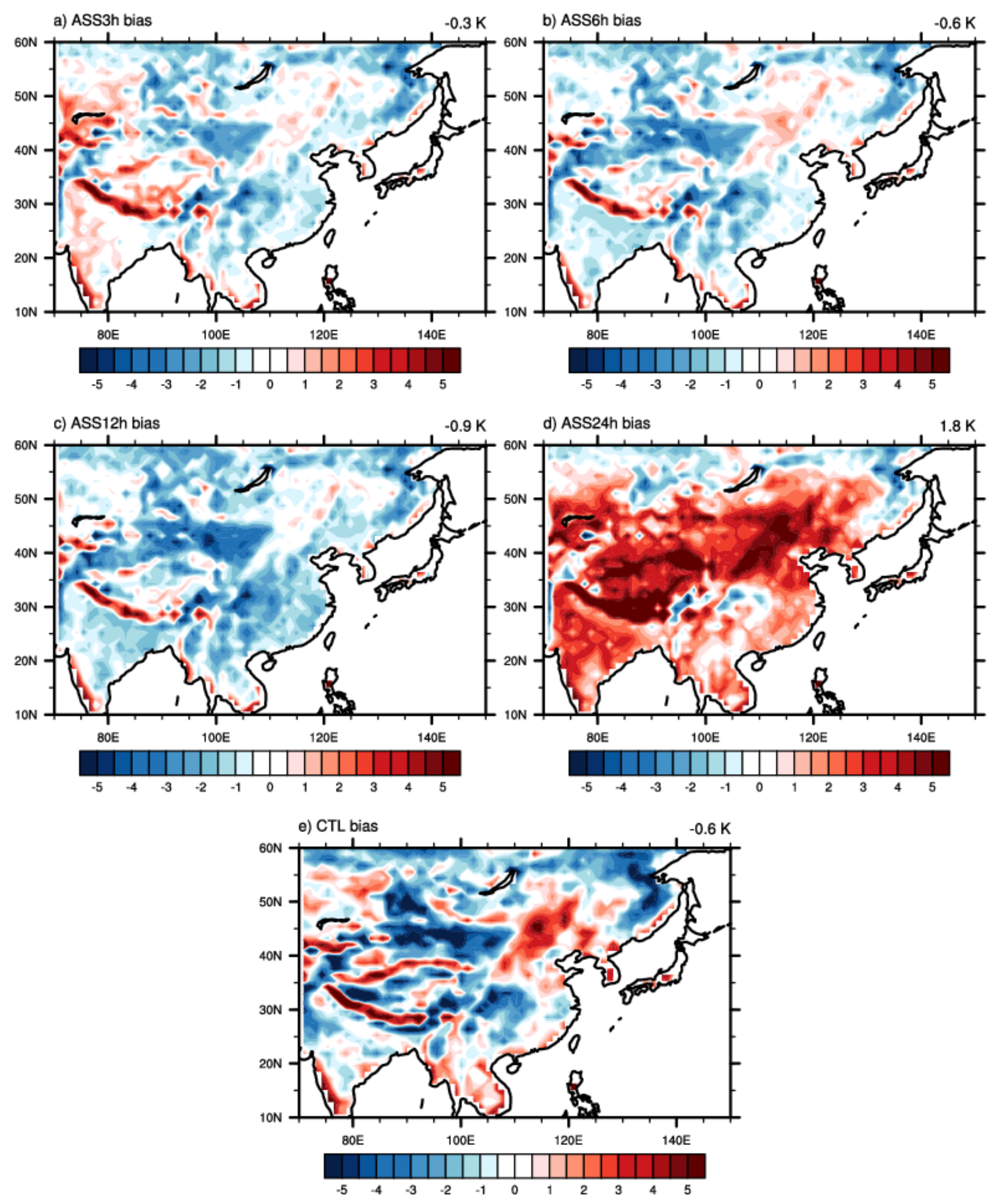
The spatial distributions of the daily-mean bias for the nighttime period of the MODIS data, the CTL experiment. and the assimilation experiments are shown in Figure 5. The regional-mean bias of the CTL experiment at nighttime is only −0.6 K and half of its daytime bias (Figure 5e). For each assimilation experiment, the biases of ASS 3 h and ASS 6 h experiments are better than that of the CTL experiment (Figure 5a,b), while the biases of ASS 12 h and ASS 24 h experiments are worse (Figure 5c,d). It can be seen that the assimilation experiments with FY-4A LST data frequencies less than 12 h have negative biases compared with the MOIDS data, while the ASS 24 h experiment reflects a positive regional-mean bias of 1.8 K. This is an interesting phenomenon, because for the FY-4A nighttime LST data, the daily-mean LST value has a significant positive bias compared with the LST during the nighttime period. The results show that when the time frequency of the FY-4A LST observations is reduced to a certain extent, the impact of diurnal variation on the simulated LST statement will significantly exceed the positive impact from assimilating FY-4A LST observations, and it can even change the overall bias pattern of the LST after assimilation.

4.3. Spatial Distribution of Time Correction

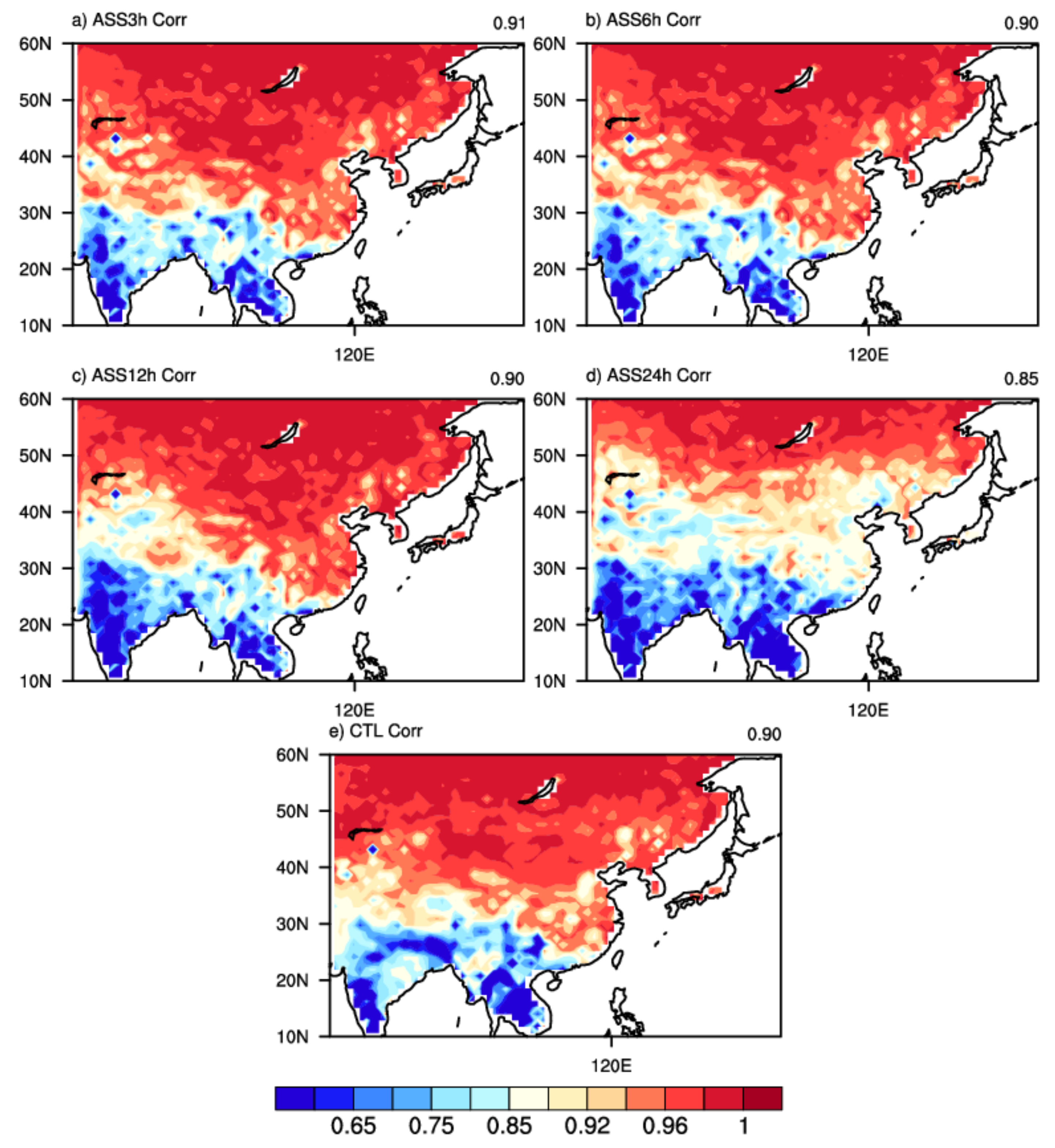
The spatial distributions of the time correlation coefficients of LST over the study period from MODIS daytime LST data, the CTL experiment, and the different assimilation experiments are shown In Figure 6. It can be cleanly seen that the time correlations exhibit a spatial distribution characteristic that increases gradually with the increase in latitude. The CTL experiment and all the assimilation experiments have better temporal consistency with the MODIS daytime LST data in areas north of 40°N, which is a semi-arid area, and the climate is dry [48]. Since there are few precipitation events in this area, the daily variability of LST is less affected by precipitation. Thus, the time variability of LST is relatively stable, and the time correlation coefficient between different LST data is high in this area. Compared with the MODIS data, the regional-mean correlation of the ASS 3 h experiment is the highest (Figure 6a) which indicates that the assimilation results can better reflect the temporal variability information of LST after increasing the time frequency of the FY-4A LST observations. On the other hand, the correlation of the ASS 24 h experiment is worse than that of the CTL experiment (Figure 6d), indicating that if the diurnal variation information of the LST data is ignored in the assimilation, the results of the correlation coefficient will be even worse than those of the CTL experiment without assimilation.
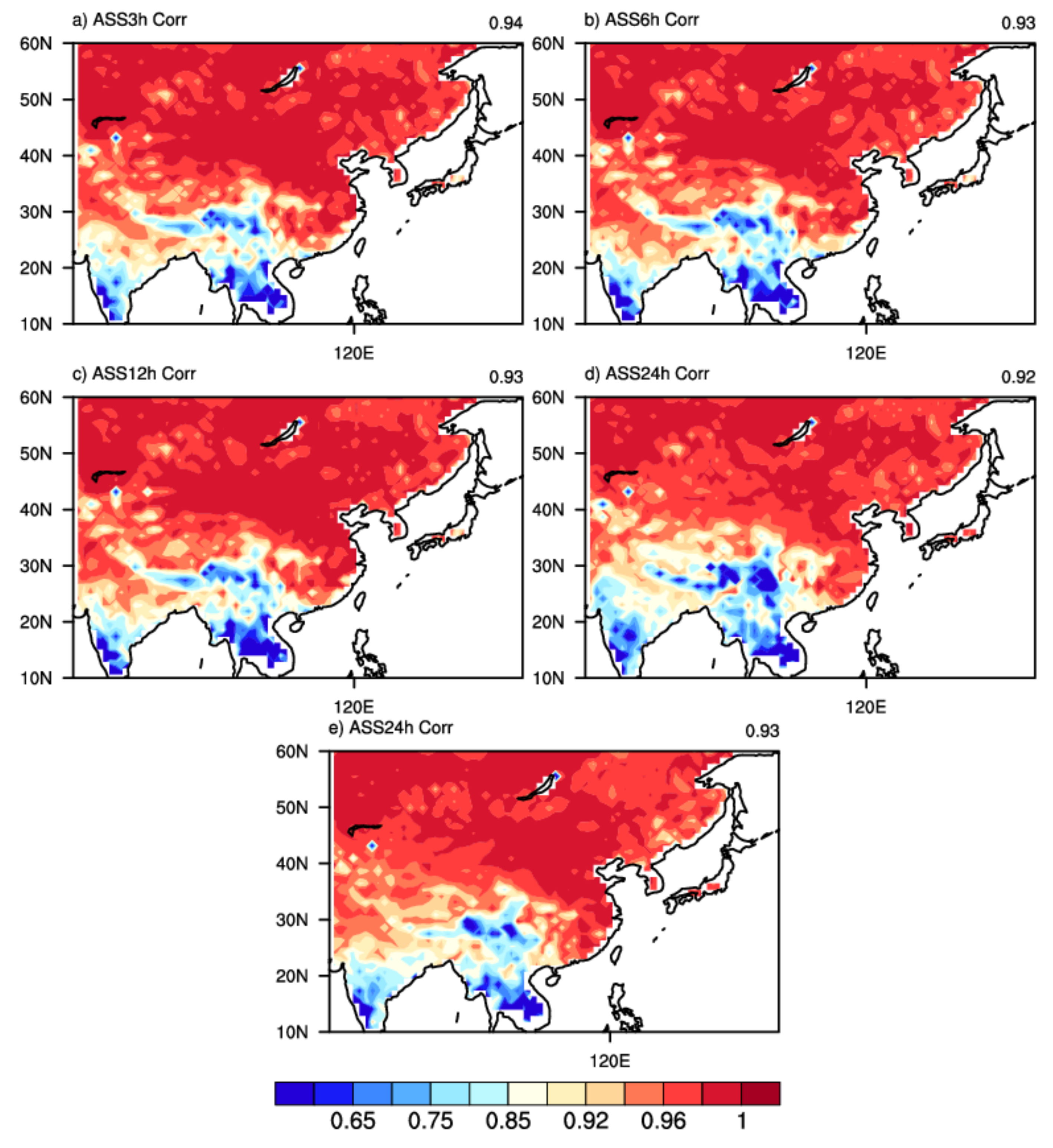
Figure 7 shows the spatial distributions of the time correlation coefficients for the MODIS nighttime data, the CTL, and different frequencies assimilation experiments. It can be seen that the spatial distribution of the time correlation at nighttime is similar to that at daytime for all those experiments. Compared with the daytime results, the time correlations of nighttime for all experiments are higher than those of the daytime experiments, which indicates that the temporal consistency of LST over the study area is better at nighttime than during daytime. When sufficient diurnal variation information is considered in the assimilation of FY-4A LST observations, the correlation of the ASS 3 h experiment is better than that of the CTL experiment (Figure 7a). When the frequency of the assimilated FY-4A observations is reduced to 6 h and 12 h, the regional averages of the correlation coefficients were the same as those of the CTL experiment (Figure 7b,c). When the observation frequencies of assimilation decrease to 24 h, the regional-mean correlation after assimilation was smaller than that of the CTL experiment due to the error caused by ignoring the diurnal variation information of LST (Figure 7d). Moreover, in can be seen that the ASS 24 h result of the nighttime is better than that of the daytime, indicating that the diurnal variation information of LST at nighttime has a smaller impact on the assimilation than that at daytime.

4.4. Spatial Distribution of RMSE

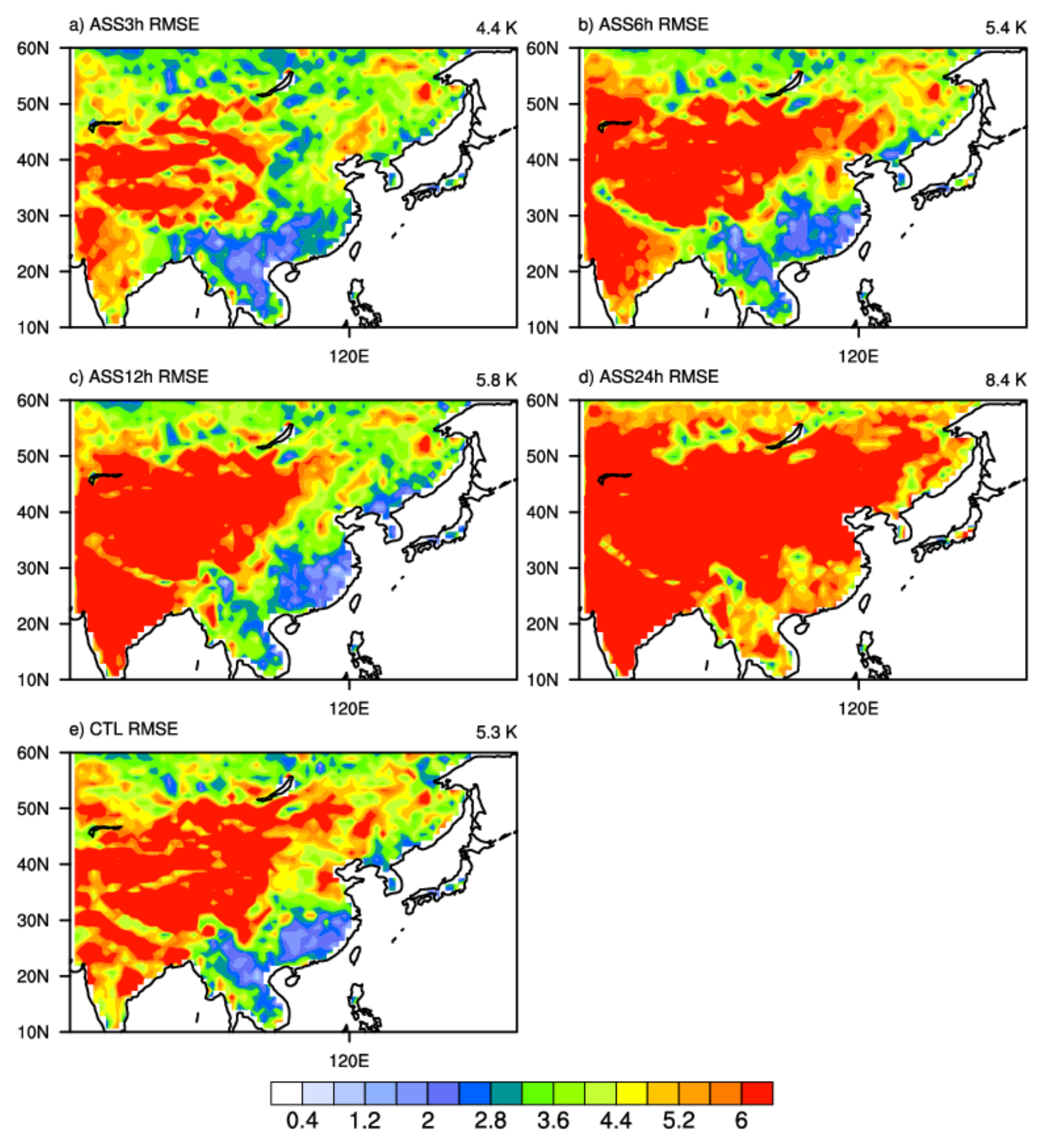
Figure 8 shows the spatial distributions of the RMSE of the CTL experiment and assimilation experiments versus the daytime MODIS data. There is an obvious large RMSE area over the western China, western Mongolia, and the Indian peninsula where the RMSE of LST can be above 6 K (Figure 8e). One possible reason for the high RMSE values in these regions is that it is generally difficult for climate models to grasp accurately the sharp warming of surface temperature over the plateau area in the daytime [44]. By comparing with the spatial pattern of the bias, this area corresponds to the large bias value area (Figure 4e); it can be considered that the large RMSE of the LST over these areas are also to some extent caused by the large biases between climate model and the MODIS daytime data. The time frequency of the FY-4A LST observations can also have a significant impact on the RMSE of the assimilation experiments. With the decrease in the time frequency of assimilated FY-4A LST data, the RMSE showed an overall increasing trend. The RMSE of the ASS 3 h experiment is smaller than that of the CTL experiment (Figure 8a), while the RMSE of other assimilation experiments with longer time frequencies are higher than that of the CTL experiment (Figure 8b–d). The difference between the RMSE and the bias magnitudes can be approximated to represent the random errors in assimilation. Comparing the results of the RMSEs and the biases for those assimilation experiments, it can be seen that this part of the random error does not change much with the decrease in the LST observation frequency. The increase in the RMSE with increasing time frequency of assimilated observation is mainly due to the system bias resulting from reduced temporal information in the FY-4A LST data.
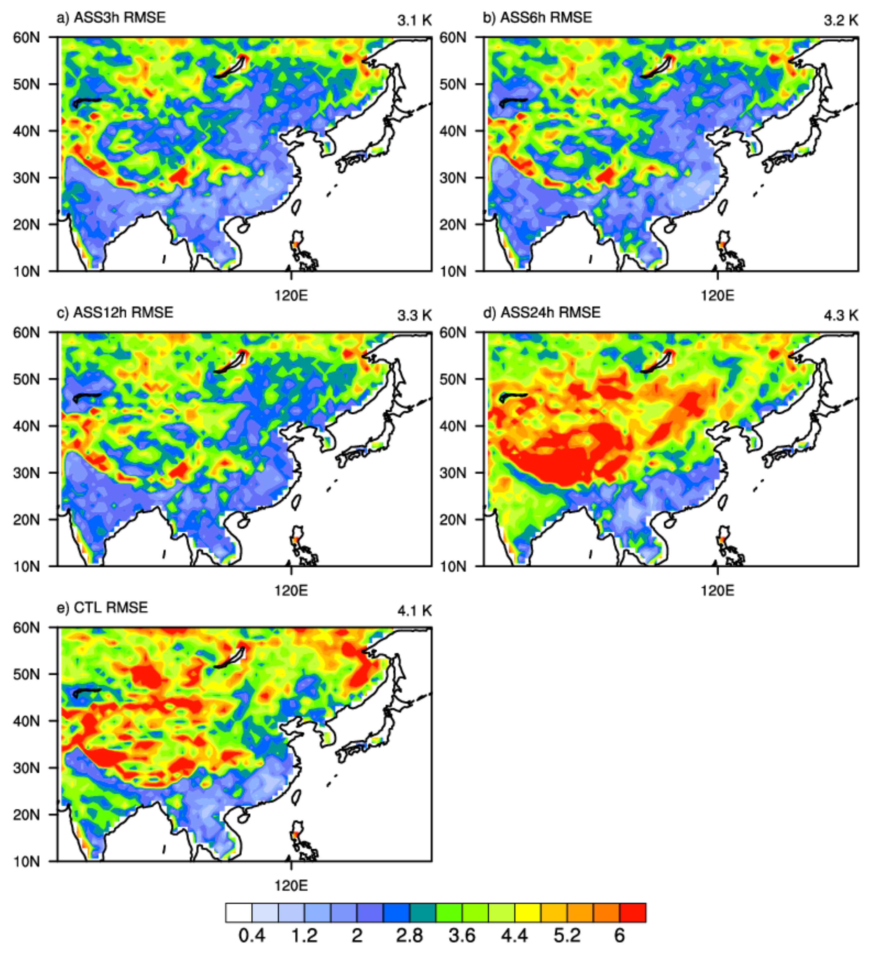
The spatial distributions of the RMSE in the nighttime period are shown in Figure 9. Compared with the daytime results, the RMSE of the CTL experiment and assimilation experiments in the nighttime period are significantly reduced. The regional-mean RMSE is 4.1 K for the CTL experiment and ranges from 3.1 K (for ASS 3 h) to 4.3 K (for ASS 24 h) for different assimilation experiments. The RMSE of the ASS 3 h, ASS 6 h, and ASS 12 h experiments is smaller than that of the CTL experiment (Figure 9a–c), while the ASS 24 h is larger (Figure 9d). This is slightly different from the bias results in which the ASS 3 h and ASS 6 h are better than the CTL and the ASS 12 h and ASS 24 h are worse but consistent with the absolute bias results (the figure was not shown). This result shows that the absolute bias makes a major contribution to the RMSE at nighttime. Moreover, if the diurnal variation of the FY-4A LST is ignored in nighttime, the RMSE of the assimilation experiment on the Tibet Plateau will increase rapidly (Figure 9d), which may be due to the fact that the plateau area has a more obvious cooling phenomenon at night than the plain area. This result suggests that the diurnal variation information is important for the assimilation of the FY-4A LST data, especially in plateau or large terrain regions.

4.5. Probability Density Function (PDF) Distribution

The PDF is another important statistic for evaluating the LST assimilation results. The PDFs of the daytime and nighttime bias, RMSE and correlation from the CTL experiment, and all assimilation experiments in all grid boxes over the study area are shown in Figure 10. The PDF distribution curves of the CTL experiments all show a left-shift phenomenon compared with the zero value in both daytime and nighttime (Figure 10a,d). All assimilation experiments also show obvious negative biases at daytime, and as the time frequency of the assimilated FY-4A LST observations decreased, the PDF curve gradually shifted to the left. The PDF distribution curves of the ASS 24 h experiment are significantly different from other assimilation experiments. The bias PDF curve of the ASS 24 h experiment has a right-shift phenomenon different from the left shift exhibited by other assimilation experiments at nighttime (Figure 10d). At daytime, the PDF curve of the ASS 24 h experiment shows an obvious double-peak phenomenon, which had a significantly stronger negative bias than assimilation experiments with shorter time frequencies. Moreover, this double-peak phenomenon also appeared in the PDF curve of RMSE, resulting in a significantly larger RMSE in the ASS 24 h experiment compared with the ASS 3 h, ASS 6 h, and ASS 12 h experiments (Figure 10b). At both daytime and nighttime, the RMSE of the ASS 3 h experiments is smaller than other assimilation experiments and the CTL experiments and has sharper PDF distribution curves. The PDF curves of the time correlation coefficients in all these experiments are similar with the peaks close to 1, and the ASS 3 h experiments show the highest correlation at both daytime and nighttime periods (Figure 10c,f).

5. Conclusions

This study assimilates the LST product with different time frequencies from the FY-4A satellite into the new BCC_AVIM2.0 land surface model. The MOD11C1 and MYD11C1 LST products derived from Terra and Aqua satellites are used to verify the assimilated results. The assessment was conducted to analyze the influence of the time frequency of FY-4A observation on the performance of the LST assimilations over the experiment region (70°E–150°E, 10°N–60°N). The main findings of this study are as follows.
  • The LST simulations of the BCC_AVIM2.0 model are lower than those of the MODIS LST products for both daytime and nighttime periods. The BCC_AVIM2.0 model significantly underestimates the LST over western China at both daytime and nighttime and overestimates it over the Indian peninsula at daytime. When the time frequency of FY-4A LST is 3 h, the ASS 3 h experiments show less biases than that of the CTL experiments at both daytime and nighttime. The biases of experiments with time intervals more than 6 h at daytime and more than 12 h at nighttime are worse than that of the CTL experiments. These large biases are due to insufficient time representativeness of the FY-4A LST data in the assimilation processes. Moreover, when the time frequency of the FY-4A LST observations is reduced to 6 h for the daytime data and 12 h for the nighttime data, the impact of diurnal variation on the simulated LST statement will significantly exceed the positive impact from assimilating FY-4A LST observations, which can even change the overall bias pattern of the LST after assimilation.
  • The RMSE of the CTL experiment and the assimilation experiments at nighttime is smaller than the corresponding experiments at daytime. The time frequency of the FY-4A LST observations can also have a significant impact on the RMSE of the assimilation experiments. With the decrease in the time frequency of assimilated FY-4A LST data, the RMSE showed an overall increasing trend at both daytime and nighttime. At nighttime, the RMSE of the assimilation experiments with time frequencies shorter than 12 h is smaller than that of the CTL experiment, while only the assimilation experiment with 3 h time frequency has a smaller RMSE than the CTL experiment. The increase in the RMSE with increasing time frequency of assimilated observation is mainly due to the system bias resulting from reduced observation time information in the FY-4A LST data.
  • In semi-arid regions where the daily variability of LST is less affected by precipitation, the CTL experiment and assimilation experiments have better temporal consistency (the time correction coefficient larger than 0.9) with the MODIS data at both daytime and nighttime. When the frequency of the assimilated FY-4A observations was reduced, the regional average correlation coefficients also decreased. After completely ignoring the diurnal variation information of LST, the ASS 24 h experiment results were even worse than that of the CTL experiments. The ASS 24 h result of the nighttime is better than that of the daytime, indicating that the diurnal variation information of LST at daytime has a larger impact on the assimilation than that at nighttime. The diurnal variation information also has an impact on the PDF distribution of the LST. The ASS 3 h experiments have sharper PDF distribution curves for RMSE than the assimilation experiments with longer LST observation frequencies. When the time frequency of the FY-4A LST observations decreases, the PDF distribution curves of the RMSE gradually shift to the right and become flat.
This study confirms the results of Fu et al. [26] that the diurnal variation information of satellite LST data is important for the assimilation of LST in climate model. Since the LST variable in nature has obvious diurnal variation characteristics, the high-frequency LST observations can better reflect the diurnal variation information of the LST, thereby better improving the diurnal variation information and the overall effect of the assimilated LST. Compared with assimilating daily frequency LST data from polar-orbiting satellites, when the assimilated LST observation frequency is increased to 6 h, the analysis error can be reduced by more than 25%. When the observation frequency is increased to more than 3 h, the analysis error can be further reduced by more than 3%. If the high-frequency variation information of LST is ignored, there will be a significant bias in the daily-mean value which can deteriorate the RMSE and temporal variability of the LST simulation. The results of this study provide a preliminary assessment of the temporal frequency of the FY-4A LST products on the performance of LST assimilation based on BCC_AVIM2.0 model. In order to obtain better assimilation results, the temporal frequency of the FY-4A LST data is suggested to be higher than 3 h for the daytime period and 6 h for the nighttime period. These results could also serve as useful feedback to the developers of the BCC_AVIM2.0 model or other land surface models, assisting them in improving the LST simulation of their models. The results of this study can also provide some suggestions for the developers of land surface data assimilation systems on improving the assimilation performance of LST data. In addition to developing more advanced assimilation methods, the application of higher frequency LST observation data is also a direction worthy of attention. This research results are also beneficial to the widely developed land-atmosphere coupling assimilation system in the future. Compared with assimilating LST data on daily or monthly scales, the assimilation of high-frequency LST data can also better improve the diurnal variation of underlying surface temperature, which will further affect the simulation and prediction of temperature, snow cover, and precipitation by the coupled climate model.

Author Contributions

Conceptualization, S.N. and X.J.; methodology, S.N.; formal analysis, Y.L. and W.C.; validation, W.D. and D.H.; investigation, L.Z.; resources, S.N. and X.J.; data curation, W.D. and X.D.; writing—original draft preparation, S.N.; writing—review and editing, X.J. and W.C.; visualization, W.D. and X.D.; supervision, D.H. and L.Z.; project administration, Y.L. and S.N.; funding acquisition, X.J. All authors have read and agreed to the published version of the manuscript.

Funding

This research was funded by the National Natural Science Foundation of China (grant nos. 42275175, 42275056 and 41801022) and the Beijing Natural Science Foundation (grant no. 8192016).

Acknowledgments

We thank the National Satellite Meteorological Center for providing the FY-4A satellite LST data. We thank the Beijing Climate Center for providing the BCC model LST data. We thank the EOS Data and Operations System (EDOS) at the Goddard Space Flight Center for providing the MODIS LST data. We thank the National Centers for Environmental Prediction (NCEP) for providing the NCEP-NCAR reanalysis data. We thank three anonymous reviewers for their helpful comments in improving this paper.

Conflicts of Interest

The authors declare no conflict of interest.

References

  1. Fuchs, M. Infrared measurement of canopy temperature and detection of plant water stress. Theor. Appl. Climatol. 1990, 42, 253–261. [Google Scholar] [CrossRef]
  2. Kustas, W.; Anderson, M. Advances in thermal infrared remote sensing for land surface modeling. Agric. For. Meteor. 2009, 149, 2071–2081. [Google Scholar] [CrossRef]
  3. Li, Z.L.; Tang, S.H.; Wu, H.; Ren, H.; Yan, G.; Wan, Z.; Trigo, I.F.; Sobrino, J.A. Satellite-derived land surface temperature: Current status and perspectives. Remote Sens. Environ. 2013, 131, 14–37. [Google Scholar] [CrossRef] [Green Version]
  4. Ghent, D.; Kaduk, J.; Remedios, J.; Ardö, J.; Balzter, H. Assimilation of land surface temperature into the land surface model JULES with an ensemble Kalman filter. J. Geophys. Res. 2010, 115, D19112. [Google Scholar] [CrossRef] [Green Version]
  5. Smith, D.; Mutlow, C.; Delderfield, J.; Watkins, B.; Mason, G. ATSR infrared radiometric calibration and in-orbit performance. Remote Sens. Environ. 2012, 116, 4–16. [Google Scholar] [CrossRef]
  6. Wan, Z. New refinements and validation of the collection-6 MODIS land-surface temperature/emissivity product. Remote Sens. Environ. 2014, 140, 36–45. [Google Scholar] [CrossRef]
  7. Muster, S.; Langer, M.; Abnizova, A.; Young, K.L.; Boike, J. Spatio-temporal sensitivity of MODIS land surface temperature anomalies indicates high potential for large-scale land cover change detection in Arctic permafrost landscapes. Remote Sens. Environ. 2015, 168, 1–12. [Google Scholar] [CrossRef] [Green Version]
  8. Norouzi, M.T.; AghaKouchak, A.; Azarderakhsh, M.; Khanbilvardi, R.; Shields, G.; Tesfagiorgis, K. Inferring land surface parameters from the diurnal variability of microwave and infrared temperatures. Phys. Chem. Earth 2015, 83–84, 28–35. [Google Scholar] [CrossRef]
  9. Didari, S.; Norouzi, H.; Zand-Parsa, S.; Khanbilvardi, R. Estimation of daily minimum land surface air temperature using MODIS data in southern Iran. Theor. Appl. Climatol. 2017, 130, 1149–1161. [Google Scholar] [CrossRef]
  10. Xu, B.; Park, T.; Yan, K.; Chen, C.; Zeng, Y.; Song, W.; Yin, G.; Li, J.; Liu, Q.; Knyazikhin, Y.; et al. Analysis of global LAI/FPAR products from VIIRS and MODIS sensors for spatio-temporal consistency and uncertainty from 2012–2016. Forests 2018, 9, 73. [Google Scholar] [CrossRef]
  11. Aumann, H.H.; Broberg, S.; Manning, E.; Pagano, T. Radiometric stability validation of 17 years of AIRS data using sea surface temperatures. Geophys. Res. Lett. 2019, 46, 12504–12510. [Google Scholar] [CrossRef]
  12. Akinyemi, F.O.; Ikanyengb, M.; Muro, J. Land cover change effects on land surface temperature trends in an African urbanizing dryland region. City Environ. Interact. 2020, 4, 100029. [Google Scholar] [CrossRef]
  13. Duan, S.B.; Li, Z.L.; Tang, B.H.; Wu, H.; Tang, R.; Bi, Y.; Zhou, G. Estimation of diurnal cycle of land surface temperature at high temporal and spatial resolution from clear-sky MODIS data. Remote Sens. 2014, 6, 3247–3262. [Google Scholar] [CrossRef] [Green Version]
  14. Reichle, R.H. Data assimilation methods in the Earth sciences. Adv. Water Resour. 2008, 31, 1411–1418. [Google Scholar] [CrossRef]
  15. Jiménez-Muñoz, J.C.; Sobrino, J.A.; Skoković, D.; Mattar, C.; Cristóbal, J. Land surface temperature retrieval methods from Landsat-8 thermal infrared sensor data. IEEE Geosci. Remote Sens. Lett. 2014, 11, 1840–1843. [Google Scholar] [CrossRef]
  16. Hain, C.R.; Anderson, M.C. Estimating morning change in land surface temperature from MODIS day/night observations: Applications for surface energy balance modeling. Geophys. Res. Lett. 2017, 44, 9723–9733. [Google Scholar] [CrossRef]
  17. Padhee, S.K.; Dutta, S. Spatiotemporal reconstruction of MODIS land surface temperature with the help of GLDAS product using kernel-based nonparametric data assimilation. J. Appl. Remote Sens. 2020, 14, 014520. [Google Scholar] [CrossRef]
  18. Amazirh, A.; Er-Raki, S.; Ojha, N.; Bouras, E.h.; Rivalland, V.; Merlin, O.; Chehbouni, A. Assimilation of SMAP disaggregated soil moisture and Landsat land surface temperature to improve FAO-56 estimates of ET in semi-arid regions. Agric. Water Manag. 2022, 260, 107290. [Google Scholar] [CrossRef]
  19. Huang, C.; Xin, L.; Ling, L. Retrieving soil temperature profile by assimilating modis lst products with ensemble kalman filter. Remote Sens. Environ. 2008, 112, 1320–1336. [Google Scholar] [CrossRef]
  20. Reichle, R.; Kumar, S.; Mahanama, S.; Koster, R.D.; Liu, Q. Assimilation of satellite-derived skin temperature observations into land surface models. J. Hydrometeorol. 2010, 11, 1103–1122. [Google Scholar] [CrossRef]
  21. Xu, T.; Liu, S.; Xu, Z.; Liang, S.; Xu, L. A dual-pass data assimilation scheme for estimating surface fluxes with FY3A-VIRR land surface temperature. Sci. China Earth Sci. 2015, 58, 211–230. [Google Scholar] [CrossRef]
  22. Chen, W.; Shen, H.; Huang, C.; Li, X. Improving soil moisture estimation with a dual ensemble Kalman smoother by jointly assimilating AMSR-E brightness temperature and MODIS LST. Remote Sens. 2017, 9, 273. [Google Scholar] [CrossRef] [Green Version]
  23. Meng, C.; Zhang, C.; Tang, R. Variational estimation of land–atmosphere heat fluxes and land surface parameters using MODIS remote sensing data. J. Hydrometeorol. 2013, 14, 608–621. [Google Scholar] [CrossRef]
  24. Shi, P.; Wang, B.; He, Y.; Lu, H.; Yang, K.; Xu, S.; Huang, W.; Liu, L.; Liu, J.; Li, L.; et al. Contributions of Weakly Coupled Data Assimilation–Based Land Initialization to Interannual Predictability of Summer Climate over Europe. J. Clim. 2022, 35, 517–535. [Google Scholar] [CrossRef]
  25. Xu, T.; Bateni, S.M.; Liang, S.; Entekhabi, D.; Mao, K. Estimation of surface turbulent heat fluxes via variational assimilation of sequences of land surface temperatures from Geostationary Operational Environmental Satellites. J. Geophys. Res. Atmos. 2014, 119, 10–780. [Google Scholar] [CrossRef] [Green Version]
  26. Lu, Y.; Steele-Dunne, S.C.; Farhadi, L.; Giesen, N. Mapping surface heat fluxes by assimilating smap soil moisture and goes land surface temperature data. Water Resour. Res. 2017, 53, 10858–10877. [Google Scholar] [CrossRef] [Green Version]
  27. Sgoff, C.; Schomburg, A.; Schmidli, J.; Potthast, R. Assimilating synthetic land surface temperature in a coupled land–atmosphere model. Q. J. R. Meteorol. Soc. 2020, 146, 3980–3997. [Google Scholar] [CrossRef]
  28. Fu, S.; Nie, S.; Luo, Y.; Chen, X. Implications of diurnal variations in land surface temperature to data assimilation using modis lst data. J. Geogr. Sci. 2020, 30, 18–36. [Google Scholar] [CrossRef] [Green Version]
  29. Yang, J.; Zhang, Z.Q.; Wei, C.Y.; Lu, F.; Guo, Q. Introducing the new generation of Chinese geostationary weather satellites, Fengyun-4. Bull. Amer. Meteor. Soc. 2017, 98, 1637–1658. [Google Scholar] [CrossRef]
  30. Min, M.; Wu, C.Q.; Li, C.; Liu, H.; Xu, N.; Wu, X.; Chen, L.; Wang, F.; Sun, F.L.; Qin, D.Y.; et al. Developing the science product algorithm testbed for Chinese next-generation geostationary meteorological satellites: Fengyun-4 series. J. Meteorol. Res. 2017, 31, 708–719. [Google Scholar] [CrossRef]
  31. Wang, T.; Luo, J.; Liang, J.; Wang, B.; Tian, W.; Chen, X. Comparisons of AGRI/FY-4A cloud fraction and cloud top pressure with MODIS/Terra measurements over East Asia. J. Meteor. Res. 2019, 33, 705–719. [Google Scholar] [CrossRef]
  32. Ge, N.; Zhong, L.; Ma, Y.M.; Fu, Y.F.; Zou, M.J.; Cheng, M.L.; Wang, X.; Huang, Z.Y. Estimations of land surface characteristic parameters and turbulent heat fluxes over the Tibetan Plateau based on FY-4A/AGRI data. Adv. Atmos. Sci. 2021, 38, 1299–1314. [Google Scholar] [CrossRef]
  33. Meng, C.; Li, H. Assimilating Satellite Land Surface States Data from Fengyun-4A. Sci. Rep. 2019, 9, 19567. [Google Scholar] [CrossRef] [PubMed] [Green Version]
  34. Chen, Y.D.; Shen, J.; Fan, S.Y.; Meng, D.M.; Wang, C. Characteristics of Fengyun-4A satellite atmospheric motion vectors and their impacts on data assimilation. Adv. Atmos. Sci. 2020, 37, 1222–1238. [Google Scholar] [CrossRef]
  35. Yin, R.; Han, W.; Gao, Z.; Di, D. The evaluation of FY4A’s Geostationary Interferometric Infrared Sounder (GIIRS) long-wave temperature sounding channels using the GRAPES global 4D-Var. Q. J. R. Meteorol. Soc. 2020, 146, 1459–1476. [Google Scholar] [CrossRef]
  36. Xia, X.; Min, J.; Shen, F.; Wang, Y.; Xu, D.; Yang, C.; Zhang, P. Aerosol data assimilation using data from Fengyun-4A, a next-generation geostationary meteorological satellite. Atmos. Environ. 2020, 237, 117695. [Google Scholar] [CrossRef]
  37. Chen, Y.; Chen, G.; Cui, C.; Zhang, A.; Wan, R.; Zhou, S.; Wang, D.; Fu, Y. Retrieval of the vertical evolution of the cloud effective radius from the Chinese FY-4 (Feng Yun 4) next-generation geostationary satellites. Atmos. Chem. Phys. 2020, 20, 1131. [Google Scholar] [CrossRef] [Green Version]
  38. Lanzante, J.R. Resistant, robust and nonparametric techniques for the analysis of climate data: Theory and examples, including applications to historical radiosonde station data. Int. J. Climatol. 1996, 16, 1197–1226. [Google Scholar] [CrossRef]
  39. Wan, Z.; Li, Z.L. A physics-based algorithm for retrieving land-surface emissivity and temperature from EOS/MODIS data. IEEE Trans. Geosci. Remote Sens. 1997, 35, 980–996. [Google Scholar]
  40. Wu, T.; Li, W.; Ji, J.; Xin, X.; Li, L.; Wang, Z.; Zhang, Y.; Li, J.; Zhang, F.; Wei, M.; et al. Global carbon budgets simulated by the Beijing Climate Center Climate System Model for the last century. J. Geophys. Res. Atmos. 2013, 118, 4326–4347. [Google Scholar] [CrossRef]
  41. Oleson, K.; Dai, Y.; Bonan, G.; Bosilovichm, M.; Dickinson, R.; Dirmeyer, P.; Hoffman, F.; Houser, P.; Levis, S.; Niu, G.-Y.; et al. Technical Description of the Community Land Model (CLM); NCAR Technical Report; University Corporation for Atmospheric Research: Boulder, CO, USA, 2004; p. 173. [Google Scholar] [CrossRef]
  42. Ji, J.J. A climate-vegetation interaction model: Simulating physical and biological processes at the surface. J. Biogeogr. 1995, 22, 2063–2069. [Google Scholar] [CrossRef]
  43. Ji, J.J.; Huang, M.; Li, K.R. Prediction of carbon exchange between China terrestrial ecosystem and atmosphere in 21st Century. Sci. China Ser. D-Earth Sci. 2008, 51, 885–898. [Google Scholar] [CrossRef]
  44. Li, W.; Zhang, Y.; Shi, X.; Zhou, W.; Huang, A.; Mu, M.; Qiu, B.; Ji, J. Development of land surface model BCC_AVIM2.0 and its preliminary performance in LS3MIP/CMIP6. J. Meteorol. Res. 2019, 33, 851–869. [Google Scholar] [CrossRef]
  45. Evensen, G. Sequential data assimilation with a nonlinear quasigeostrophic model using Monte Carlo methods to forecast error statistics. J. Geophys. Res. 1994, 99, 10143–10162. [Google Scholar] [CrossRef]
  46. Kalman, R.; Bucy, R. New results in linear prediction and filtering theory. Trans. AMSE J. Basic Eng. 1961, 83D, 95–108. [Google Scholar] [CrossRef] [Green Version]
  47. Burgers, G.; van Leeuwen, P.J.; Evensen, G. Analysis scheme in the ensemble Kalman filter. Mon. Weather Rev. 1998, 126, 1719–1724. [Google Scholar] [CrossRef]
  48. Deng, X.; Nie, S.; Deng, W.; Cao, W. Statistical evaluation of the performance of gridded monthly precipitation products from reanalysis data, satellite estimates, and merged analyses over China. Theor. Appl. Climatol. 2018, 132, 621–637. [Google Scholar] [CrossRef]
Figure 1. Flow chart of the FY-4A LST assimilation strategy.
Remotesensing 15 00059 g001
Figure 2. The spatial distributions of the daytime annual mean LST (K) for the assimilation experiments with (a) 3 h, (b) 6 h, (c) 12 h, (d) 24 h time frequencies, (e) the CTL experiment, and (f) the MODIS data.
Remotesensing 15 00059 g002
Figure 3. Same as in the Figure 2 but for the nighttime data.
Remotesensing 15 00059 g003
Figure 4. The spatial distributions of the daytime daily-mean LST bias (K) versus the MODIS data for the assimilation experiments with (a) 3 h, (b) 6 h, (c) 12 h, and (d) 24 h time frequencies and (e) the CTL experiment.
Remotesensing 15 00059 g004
Figure 5. Same as in the Figure 2 but for the nighttime data.
Remotesensing 15 00059 g005
Figure 6. The spatial distributions of the time correlation coefficients between the LST of (a) the ASS 3 h experiment, (b) the ASS 6 h experiment, (c) the ASS 12 h experiment, (d) the ASS 24 h experiment, and (e) the CTL experiment and the daytime MODIS data.
Remotesensing 15 00059 g006
Figure 7. Same as in the Figure 6 but for the nighttime data.
Remotesensing 15 00059 g007
Figure 8. The spatial distributions of the RMSE (K) between the LST of (a) the ASS 3 h experiment, (b) the ASS 6 h experiment, (c) the ASS 12 h experiment, (d) the ASS 24 h experiment, and (e) the CTL experiment and the daytime MODIS data.
Remotesensing 15 00059 g008
Figure 9. Same as in the Figure 8 but for the nighttime data.
Remotesensing 15 00059 g009
Figure 10. The PDFs of the bias (a,d), the RMSE (b,e), and the time correlation coefficient (c,f) for the CTL experiments and the assimilation experiments at daytime (left column) and nighttime (right column) periods.
Remotesensing 15 00059 g010
Disclaimer/Publisher’s Note: The statements, opinions and data contained in all publications are solely those of the individual author(s) and contributor(s) and not of MDPI and/or the editor(s). MDPI and/or the editor(s) disclaim responsibility for any injury to people or property resulting from any ideas, methods, instructions or products referred to in the content.