Combining Environmental, Multispectral, and LiDAR Data Improves Forest Type Classification: A Case Study on Mapping Cool Temperate Rainforests and Mixed Forests

Abstract

Predictive vegetation mapping is an essential tool for managing and conserving high conservation-value forests. Cool temperate rainforests (Rainforest) and cool temperate mixed forests (Mixed Forest, i.e., rainforest spp. overtopped by large remnant Eucalyptus trees) are threatened forest types in the Central Highlands of Victoria. Logging of these forest types is prohibited; however, the surrounding native Eucalyptus forests can be logged in some areas of the landscape. This requires accurate mapping and delineation of these vegetation types. In this study, we combine niche modelling, multispectral imagery, and LiDAR data to improve predictive vegetation mapping of these two threatened ecosystems in southeast Australia. We used a dataset of 1586 plots partitioned into four distinct forest types that occur in close proximity in the Central Highlands: Eucalyptus, Tree fern, Mixed Forest, and Rainforest. We calibrated our model on a training dataset and validated it on a spatially distinct testing dataset. To avoid overfitting, we used Bayesian regularized multinomial regression to relate predictors to our four forest types. We found that multispectral predictors were able to distinguish Rainforest from Eucalyptus forests due to differences in their spectral signatures. LiDAR-derived predictors were effective at discriminating Mixed Forest from Rainforest based on forest structure, particularly LiDAR predictors based on existing domain knowledge of the system. For example, the best predictor of Mixed Forest was the presence of Rainforest-type understorey overtopped by large Eucalyptus crowns, which is effectively aligned with the regulatory definition of Mixed Forest. Environmental predictors improved model performance marginally, but helped discriminate riparian forests from Rainforest. However, the best model for classifying forest types was the model that included all three classes of predictors (i.e., spectral, structural, and environmental). Using multiple data sources with differing strengths improved classification accuracy and successfully predicted the identity of 88% of the plots. Our study demonstrated that multi-source methods are important for capturing different properties of the data that discriminate ecosystems. In addition, the multi-source approach facilitated adding custom metrics based on domain knowledge which in turn improved the mapping of high conservation-value forest.

1. Introduction

Effective management of high conservation-value ecosystems depends on an accurate accounting of where these ecosystems occur and how abundant they are. In forested landscapes, mapping of vegetation types has long been the standard approach to delineate areas of conservation importance. This provides a benchmark for monitoring long-term changes in abundance [1], as well as a practical tool to avoid inadvertent anthropogenic impacts (e.g., land clearance, logging) on protected vegetation types. A key component of predictive vegetation mapping is the ability to discriminate between different forest communities or stand types across broad spatial scales. Structurally and compositionally complex forests can present a challenge for forest classification using environmental modeling and remote sensing. This is especially true when forest types might vary locally based on bushfire, timber harvesting, and historical land-use legacies, leading to heterogeneous distributions of forest types within the landscape [2].

In the fire-prone landscapes of southeast Australia [3], rainforest ecosystems are restricted to the cooler and wetter areas of the landscape where fire is infrequent [2,4,5]. Cool temperate rainforests (hereafter called Rainforest) are considered endangered due to widespread loss due to land clearing and the effects of fire and timber harvesting. Cool temperate mixed forest (hereafter called Mixed Forest) is considered an intermediate stage in the transition of wet sclerophyll forest to Rainforest, typically occurs adjacent to Rainforest, and is subject to similar threats [6]. Fedrigo et al. [7] referred to Mixed Forest as an ecotonal stand type that is structurally and compositionally distinct from Rainforest and eucalypt forests. Despite being recognized as a distinct ecological vegetation class (EVC), Mixed Forest have not been formally mapped due to difficulties in demarcating rainforest species in the understorey below a eucalypt canopy using aerial imagery [8]. Fedrigo et al. [9] utilized Light Detection and Ranging (LiDAR) data to map the occurrence of Rainforest based on structural characteristics. Intermediate Rainforest-modeled probabilities (40 to 59%) were considered as potential Mixed Forest areas. However, the ability to discriminate between rainforest and non-rainforest species with similar structural characteristics was limited because only LiDAR data were included in the analyses. Fedrigo et al. [1] combined LiDAR data with species distribution models and satellite estimates of vegetation cover to provide the first Mixed Forest predictions for the region. However, due to discrepancies between the predicted occurrence of rainforest indicator species and their actual occurrence (i.e., the latter being a subset of the predicted occurrence) and overlaps in the predicted niches of non-rainforest and rainforest species, the model tended to overestimate the current extent of Mixed Forest. Despite these limitations, the work of Fedrigo et al. [1] highlighted the value of using different groups of predictors to make spatial predictions of forest types at broad spatial scales.

Habitat suitability models (HSMs, also known as species distribution- or niche-models) are based on niche theory, which states that a species’ distribution is limited by its fundamental niche [10,11]. The fundamental niche is the range of environmental conditions in which a species is able to grow and survive in the absence of biotic constraints (e.g., competition, predation). Climatic predictors are usually able to inform the broad geographic distribution of a species, while topographic features can help predict its occurrence at finer scales. Habitat suitability models are useful for mapping and understanding the environmental requirements of a species or a community assemblage. They have been used extensively to map rare species [12,13,14], guide conservation [15,16], and forecast the effect of climate change on vegetation [17,18,19]. In the forestry literature alone, there have been over 350 papers published using HSMs for different purposes between 2000 and 2019 [20]. Part of the popularity of HSMs is likely due to the wide availability of presence/absence—and to an even greater extent presence-only—data and the simplicity of calibrating the models due to the widespread availability of environmental predictor maps and the development of HSM software and libraries.However, in practice, there are different reasons why a species might be present or absent from a site. Competition, dispersal limitation, allogenic (e.g., fire) and/or biogenic factors (e.g., disease) can all prevent a species from occurring at a site or in a region [10,21]. Together these processes typically lead to a species occupying a subset of its fundamental niche. This is known as the realised niche. Disentangling the fundamental niche from the realised niche has been a criticism of HSMs for more than a decade [22]. For predictive ecosystem mapping, this can lead to species being mapped to where they can occur, not where they do occur (see [1]). Creating high-resolution predictive maps of actual—rather than potential—species’ locations requires additional information based on direct measurement at the landscape scale.

The development of satellite sensors in the 1970s (notably Landsat) has driven rapid growth in the use of multispectral analysis for large-scale land classification [23], vegetation [24,25], and forest type mapping [26]. Multispectral imagery provides a direct measure of the reflectance properties of objects, which can be used to discriminate species and forest types that have different spectral reflectances. For example, the spectral reflectance of conifer species is distinct from that of angiosperm species, allowing these groups to be readily distinguished from each other [27]. Hyperspectral methods provide finer spectral resolution than multispectral imagery; however, they have not been widely adopted for landscape classification as readily accessible datasets are rare for broad-scale studies. An important constraint of spectral imagery is that it is mostly limited to measuring the upper canopy of a forest (although see Eriksson et al. [28]). It is unable to measure understorey vegetation below a dense forest canopy. This hampers its ability to discriminate forest types that share the same overstorey but have different understorey structures and/or compositions. This situation occurs in the temperate wet forests of southeast Australia, where tall wet Eucalyptus forests and Mixed Forest are both dominated by a canopy of Eucalyptus spp. but have distinct understorey compositions [7]. Discriminating forest types with these characteristics requires specific tools that can detect differences in stand structure.

Measuring stand structure is a strength of LiDAR remote sensing tools. LiDAR allows for the acquisition of three-dimensional point clouds of scanned areas. The point cloud can then be used to derive LiDAR metrics that can help describe stand structure [29,30] and identify tree species [31]. Fedrigo et al. [9] utilized LiDAR to discriminate between Rainforest and Eucalyptus stands in southeast Victoria based on plant area volume density profiles derived from airborne LiDAR. Other common LiDAR metrics include the maximum point height in each pixel, the proportion of LiDAR points reaching the ground, or the proportion of LiDAR points in different height classes.

While many studies have used one of the approaches described above, there is a growing literature highlighting the benefits of combining multiple approaches, particularly those that integrate spectral imagery, structural metrics, and environmental predictors [32]. Model-based inventory [33] can be utilized to connect different forest types with multiple predictors representing environment, reflectance, and structure through supervised learning. In the Central Highlands of Victoria in southeast Australia, montane forests occur in complex, heavily dissected landscapes in which forest structure and composition are influenced by climate, topography, and infrequent but severe bushfires [3,34,35]. This has largely resulted in Rainforest occurring in gullies surrounded by wet Eucalyptus forests [36]. On the flanks of these gullies, Mixed Forest develops in areas where bushfires have not occurred in the last 100 years or more [7,37]. The high conservation values of Rainforest and Mixed Forest have afforded these communities protection from timber harvesting; however, the lack of robust mapping of Mixed Forest means its extent and condition is uncertain, with preliminary analysis suggesting a minimum ‘rare’ Bioregional Conservation Status [38]. Identifying where Rainforest and Mixed Forest currently occur is critical for setting baseline information for monitoring their conservation status over time.

The primary goals of this study were to (1) map high conservation-value forest types (i.e., Rainforest and Mixed Forest) in the Central Highlands of Victoria and (2) quantify how well environmental, spectral, and LiDAR datasets are able to predict the occurrence of these forest types within a broader landscape mosaic of eucalypt forests.

2. Materials and Methods

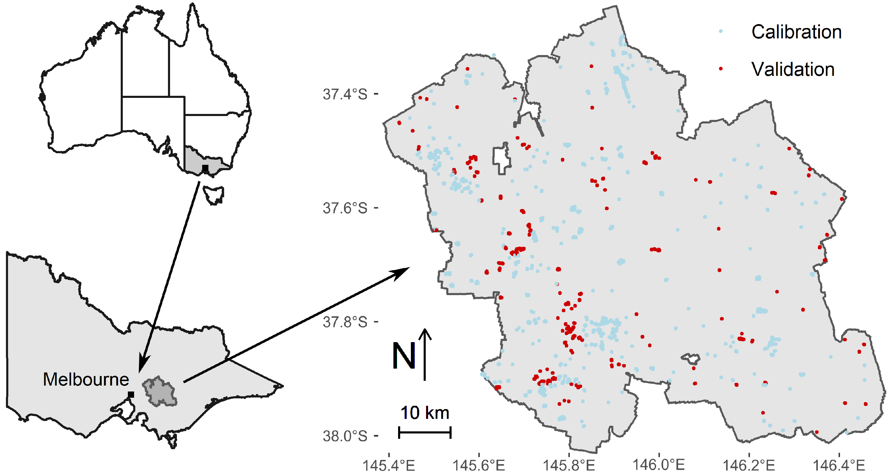
2.1. Study Area

2.1.1. The Central Highlands of Victoria

Our study area is the Central Highlands of Victoria, a mountainous region ∼80 km east of Melbourne in southeast Australia (Figure 1). The Central Highlands range from 300 to 1800 m above sea level and contain a diverse range of vegetation types. However, the dominant vegetation is eucalypt forests interdigitated with Rainforest and Mixed Forest that have high conservation values. A key tenet of sustainable management of the region’s forest is the protection of forest types with high conservation values; however, this requires accurate maps of their distribution. As part of the renewal of the Victorian Regional Forest Agreements for the 2020–2035 period, the Victorian government committed to updating its mapping of high conservation-value forests, including Rainforest and Mixed Forest. The mapping of Rainforest currently used in Victoria is based on EVC modelling (encompassing many other vegetation types, see https://www.environment.vic.gov.au/biodiversity/bioregions-and-evc-benchmarks (accessed on 10 October 2022)), which is useful for its broad description of the landscape but lacks the precision required for tactical or operational planning and conservation. The mapping of Mixed Forest was stipulated in the 1998 Central Highlands Forest Management Plan [39] but has yet to be completed.

2.1.2. Cool Temperate Rainforests

Cool temperate rainforests are closed-canopy, non-eucalypt forests occurring in high rainfall areas protected from fire (gullies) within wet forests. The overstorey species indicative of rainforests are Nothofagus cunninghamii (myrtle beech) and Atherosperma moschatum (sassafras). Additional species such as Acacia melanoxylon and A. dealbata are also common in these forests. The understorey is characterized by the presence of tree ferns (Cyathea australis and Dicksonia antarctica), which host a rich epiphytic flora [40,41,42]. In Victoria, Rainforest is defined as a forest with (1) the occurrence of Nothofagus cunninghamii or Atherosperma moschatum, (2) at least 70% projected foliage cover of Nothofagus cunninghamii, Atherosperma moschatum, Acacia melanoxylon, and A. dealbata, and (3) less than 10% Eucalyptus cover.

2.1.3. Cool Temperate Mixed Forests

Cool temperate mixed forest is characterized by Rainforest with a sparse overstorey of Eucalyptus spp. Mixed Forest contains at least 70% projected foliage cover of rainforest species and more than 10% Eucalyptus cover [43]. These are typically ecotones between eucalypt forests and Rainforest and are considered to hold high conservation because of the presence of rainforest species in the understorey layer.

2.1.4. Other Forest Types

While eucalypt forest, Rainforest, and Mixed Forest account for almost all of the forest area in the Central Highlands, there are other forest types of varying composition and distribution. Tree fern species in the Central Highlands, and often found in Rainforest, but are not considered obligate rainforest species. Areas dominated by tree ferns, including tree fern stands mixed with non-obligate rainforest species such as Leptospermum spp. (tea tree), were categorized for simplicity as “Fern” stands. In this landscape, Fern stands are not considered as a high conservation-value forest type [42].

All other forests (i.e., not characterized as Rainforest, Mixed Forest, or Fern) were classified as eucalypt forest (‘Euc’). While some of these areas might also include other tree species (e.g., Acacia spp.), they are relatively common and less important from a conservation perspective. Definitions and acronyms used for the four modelled forest types are summarized in

Table 1. Modelled forest type definitions.

Forest Type Code	Definition
Rainforest	Cool temperate rainforest. Area with more than 70% projective foliage cover of rainforest species and less than 10% of Eucalyptus spp.
Mixed Forest	Cool temperate mixed forest. Area with more than 70% projective foliage cover of rainforest species and more than 10% Eucalyptus spp.
Fern	Fern-dominated stands. Fern stands are sometimes accompanied by scrubs.
Euc	Primarily Eucalyptus-dominated stands but includes everything that is not classified as Rainforest, Mixed Forest, or Fern.

.

2.2. Field-Based Forest Type Assessment

The data used to train and test our model to classify forest types came from three sources:

1.

Plot data were collected from several previous research projects. Based on the biometric inventory of the plots (i.e., species, diameter at breast height, crown width, crown cover, etc.), we categorized plots as Euc, Mixed Forest, and Rainforest (None of these Stage 1 plots met the criteria for the Fern type). We used Nearmap (https://www.nearmap.com/au/en (accessed on 8 December 2021)) and LiDAR canopy height models to address potential GPS inaccuracies (the GPS coordinates had ∼20 m accuracy) associated with plot location. Plots that had a mismatch between field observations and nearmap were relocated within their 20 m surrounding area to match the forest type that was observed in the field. At this step, we also filtered plots from the same forest type that were less than 100 m from each other to avoid small-scale spatial autocorrelation issues. Stage 1 plots are the dominant source of ground-based data for this research.

2.

Under-sampled areas of the Central Highlands (e.g., this was the case in the eastern part of the region in Figure 1) were identified and additional field data were collected. Clusters of three plots were identified in a prototype model as Rainforest, Mixed Forest, and Euc forest types in areas that lacked samples and confirmed by site visits.

3.

To avoid classifying areas with only tree fern canopies as Rainforest areas, we used high resolution (7.5 cm) aerial photos to create data points for the Fern forest type category. The star shape and bright green colouration of tree fern stands made them easy to distinguish from the other forest types based on aerial photography alone.

In total, a database of 1586 plots was developed including 769 Euc, 156 Fern, 356 Mixed Forest, and 305 Rainforest plots.

2.3. Environmental Predictors

Based on preliminary analysis, four bioclimatic variables were considered to discriminate the broad-scale distribution of the four forest types: annual mean temperature (bio01), isothermality (bio03), temperature seasonality (bio04), and annual precipitation (bio12) (

Table 2. Predictor description. The ‘group’ column represents the different group of predictors that we used in our analysis (i.e., environmental, multispectral, and LiDAR predictors), the ‘predictor’ column is the name associated with each predictor, the ‘description’ column provides a brief description of each predictor, and the ‘resolution’ column shows the spatial resolution of the different predictors.

Group	Predictor	Description	Resolution (m)
Environmental	Creek index	Gully index. Higher values indicate the presence of gullies	20
	bio01	Mean annual temperature	20
	bio01_2	Squared bio01	20
	bio03	Isothermality (ratio of mean diurnal range (Mean of monthly (max temp-min temp)) to temperature annual range)	20
	bio03_2	Squared bio03	20
	bio04	Temperature Seasonality (standard deviation of monthly mean temperature)	20
	bio04_2	Squared bio04	20
	bio12	Mean annual precipitation	20
	bio11_2	Squared bio12	20
Multispectral	Red_edge	Pan-sharpened (with red band as hi-res) red-edge (Sentinel band 5, 705 nm)	20
	Green/Red	Simple ratio of Sentinel Band 3 (green, 560 nm) with Sentinel Band 4 (red, 665 nm)	20
	Green/NIR1	Simple ratio of Sentinel Band 3 (green, 560 nm) with sentinel Band 6 (near IR1, 740 nm)	20
	Green/NIR2	Simple ratio of Sentinel Band 3 (green, 560 nm) with sentinel Band 7 (Near IR 2, 783 nm)	20
	Green/NIR3	Simple ratio of Sentinel Band 3 (green, 560 nm) with Sentinel Band 8 (Near IR 3, 842 nm)	20
	Green/NIR4	Simple ratio of Sentinel Band 3 (green, 560 nm) with sentinel Band 8a (Near IR 4, 865 nm)	20
	Blue/Green	Simple ratio of Sentinel Band 2 (blue, 490 nm) with sentinel Band 3 (Green, 560 nm)	20
	TNGRDI	Normalized green-red difference index 32 years Landsat composite: $TNGRDI=\frac{\frac{ban{d}_{2,q75}}{ban{d}_{3,q75}}-\frac{ban{d}_{2,q25}}{ban{d}_{3,q25}}}{\frac{ban{d}_{2,q75}}{ban{d}_{3,q75}}+\frac{ban{d}_{2,q25}}{ban{d}_{3,q25}}}$	25
LiDAR	p10, p25, p50, and p90	10th, 25th, 50th and 90th percentiles of point return height (m)	20
	s00 to s60	Percentage of all LiDAR point returns in 5 m height classes (%)	20
	pfc	Percentage of first returns (i.e., percentage forest cover)	20
	ovnum	Number of overstorey trees with crown width > 8 m	20
	ovcwavg	Average overstorey tree crown width (in m)	20
	mscover	Percentage cover of midstorey trees	20
	msnum	Number of misdtorey trees	20
	mshtavg	Average midstorey tree height	20
	pavd_PC1–pavd_PC9	First to ninth PCA component of PAVD	20

). These bioclimatic variables are averages for the 1980–2014 period and were extracted using the raster package [44] in R. The initial climatic data had a 250 × 250 m resolution [45]. We used kriging interpolation to resample the climatic data to a 20 × 20 m resolution [46] to match the resolution of our remote-sensing predictors. To allow for the bell-shaped response curve typically found in HSMs, we added a quadratic transformation of the bioclimatic variables as a predictor to our model.

We also included a local topographic predictor. The creek index was calculated from the LiDAR-derived digital elevation model for the area and represents the topographic position of each 20 × 20 m pixel in the catchment. Since Rainforest, and to a lesser degree Mixed Forest and Ferns, are typically associated with gullies and Eucalyptus forests are associated with slopes and ridges, we expected the creek index to help discriminate amongst these forest types.

2.4. Multispectral Predictors

We used Sentinel-2 satellite data to develop multi-spectral predictors useful for characterizing vegetation type. The Sentinel-2 earth observation satellite collects reflectance data in 13 spectral bands ranging from ultra-blue (∼443 nm) to shortwave infrared (∼2190 nm) at pixel resolutions ranging from 10 to 60 m. Using the Google Earth Engine platform (GEE), a composite mosaic for the study area was created from the median of each of Sentinel bands 2–8, 8a, 11 and 12 (see, https://sentinels.copernicus.eu/web/sentinel/technical-guides/sentinel-2-msi/msi-instrument (accessed on 8 December 2021)) at each pixel, obtained from the cloud and cloud shadow-free set of images obtained over the 2017–2018 summer season. We used bilinear interpolation to resample Sentinel-2 bands (2, 3, 4, and 6) from a 10 to a 20 m resolution to match the spatial resolution of the other predictors.

Several of the standard vegetation indices, including Normalized Difference Vegetation Index (NDVI), Green Normalized Difference Vegetation Index (GNDVI), Enhanced Vegetation Index (EVI) and Normalized Difference Moisture Index (NDMI), were trialled as part of another rainforest modelling and mapping project conducted across the same region [8]. While these indices proved useful, they did not perform as well as simple band ratios for the task of delimiting narrow strips of mesophyll rainforest from the surrounding Eucalypt dominated sclerophyll forest in the study area. For this reason, we used the simple band ratios identified in White et al. [8] as predictors in our analysis (Table 2).

A critical determinant of the presence of rainforest in South-Eastern Australia is the long-term absence of wildfire and other disturbance associated with timber harvesting. To inform the modelling of past forest disturbances that may indicate past loss of rainforest or mixed forest, we created a composite variable from the 32-year long Landsat platform dataset. Using GEE, we obtained both the 25th and 75th percentile for each of Landsat band 2 (Green) and Landsat band 3 (Red) for all cloud shadow-free images captured during all summer months between 1987 and 2016. We then used a difference approach to highlight vegetation perturbation within the 32-year chronosequence revealed by the temporally normalized difference red/green index (TNDRGI, see Table 2 for the derivation of the variable).

2.5. LiDAR Predictors

We used forest structure metrics developed from LiDAR data to help discriminate among forest types. To match the resolution of the satellite imagery predictors, we used a 20 × 20 m planimetric resolution for the LiDAR-derived predictors.

2.5.1. LiDAR Raw Data

Discrete return airborne LiDAR data were acquired by RPS Group Plc in late 2015 and early 2016 using a Trimble AX60 laser sensor mounted on a fixed-wing aircraft. The aircraft was flown at 800 m above the ground with a flying speed of 62 m/s. The LiDAR data covered 464,716 hectares of the Victorian Central Highlands and the dataset was cut into 4647 1 × 1 km tiles. The average point cloud density over the region was 28.1 points per m${}^2$. Data were normalized to ground using the data provider’s digital elevation model which was computed on the same LiDAR dataset.

2.5.2. Standard Area-Based LiDAR Metrics

We used several common LiDAR metrics from the FUSION software [47] to describe the structure of the vegetation in each pixel. This included the ratio between the number of first returns and total returns (pfc, a proxy for percentage forest cover [48]), the percentage of point returns in each 5 m height classes, and different percentiles of LiDAR return heights.

2.5.3. LiDAR Metrics Based on Individual Tree Detection

The results of a previous project that delineated individual tree crowns (ITD) in the region based on the same LiDAR dataset [46] gave us the opportunity to test the influence of ITD metrics on forest type classification. Specifically, we used the estimated number of large overstorey trees (>8 m crown diameter) and the average overstorey crown width as predictors in our study. We expected these metrics to be particularly useful for discriminating Rainforest from Mixed Forest as Mixed Forest are essentially rainforest species overtopped by large remnant Eucalyptus trees. Ruizhu [46] also calculated midstorey metrics based on ITD (e.g., number and average height of the midstorey per pixel, and midstorey cover), which we also incorporated as predictors in our study.

2.5.4. Plant Area Volume Density Predictors

Another study in the region [9] showed that metrics based on plant area volume density profiles (PAVD) were useful predictors of rainforest presence. We followed the workflow described in Fedrigo et al. [9] to extract PAVD predictors for each of our 1586 plots. We first calculated PAVD values for each pixel with a 1-m height resolution. We then used principal component analysis (PCA) of the 80 PAVD height classes based on our field dataset to extract the most important signals of the structural profile. Finally, we selected the nine most important components of the PCA as predictors as in Fedrigo et al. [9]. These nine principal components captured 87% of the variance in the data. PCA loadings are provided in Supplementary Materials S1.

A summary description of the 45 predictors (49 when the quadratic terms for the bioclimatic predictors are included) used in this study is available in Table 2.

2.6. Statistical Models

We used Bayesian generalized linear models with a categorical error distribution (i.e., a generalization of the Bernoulli distribution for more than two categories) and a softmax link (i.e., a generalization of the logit link for more than two categories) to model our four forest-type categories. The softmax (sometimes called multinomial logit) function takes a vector of latent scores s, one for each of our four categories k, and computes the probability of a particular type of category as:

$$\mathrm{Pr}\left(k\right)=\frac{exp\left(s_k\right)}{{\sum }_{i=1}^{4}exp\left(s_i\right)}$$

(1)

where the probability of predicting target category k depends on the value of the exponential score $s_k$ relative to the score for the other categories. Since the probability associated with the prediction at each plot has a sum-to-one constraint (i.e., if we know the probability of any three categories, we can deduce the probability for the fourth category), only three latent scores per plot need to be estimated. To solve for this identifiability issue, it is common practice to set the latent score value of the reference category (in our case Euc) to zero.

The latent scores for the three other categories are modelled as a linear function of the predictors:

$$\begin{array}{cc}\hfill s_{\mathrm{Euc}}& =0\hfill \\ \hfill s_{\mathrm{Fern}}& ={\alpha }_{\mathrm{Fern}}+{\beta }_{\mathrm{Fern}}X\hfill \\ \hfill s_{\mathrm{Mixed}\mathrm{Forest}}& ={\alpha }_{\mathrm{Mixed}\mathrm{Forest}}+{\beta }_{\mathrm{Mixed}\mathrm{Forest}}X\hfill \\ \hfill s_{\mathrm{Rainforest}}& ={\alpha }_{\mathrm{Rainforest}}+{\beta }_{\mathrm{Rainforest}}X\hfill \end{array}$$

(2)

where ${\alpha }_{\mathrm{Fern}}$, ${\alpha }_{\mathrm{Mixed}\mathrm{Forest}}$ and ${\alpha }_{\mathrm{Rainforest}}$ are the intercepts associated with each forest type; ${\beta }_{\mathrm{Fern}}$, ${\beta }_{\mathrm{Mixed}\mathrm{Forest}}$ and ${\beta }_{\mathrm{Rainforest}}$ are slope parameter vectors of length 49 associated with the 49 predictors (for the Full model); and X is the predictor matrix. The Full model has 150 parameters (each of the three forest type having 50 parameters, and the latent score for Euc being fixed to zero).

Since we had many predictors but only expected a handful of them to be of importance for model predictions, we used regularized methods, specifically horseshoe priors, to estimate our parameters [49,50]. Horseshoe priors have the tendency to shrink parameters toward zero if the effect of the predictor associated with this parameter is negligible, while being relatively neutral for parameters that are associated with strong variables. This can be especially useful to stabilize parameter values and simplify model interpretability when using many potential predictors. However, since regularization penalizes models for large parameters, it is necessary for the parameters to be on the same scale. For this reason, predictors were scaled to have a mean of zero and a standard deviation of one prior to model fitting. Scaling also has the advantage of putting all parameters on the same scale to facilitate parameter interpretation (i.e., the effect size associated with each parameter can be used as a metric of variable importance).

To test for the influence of predictor group on our ability to discriminate different forest types, we fitted five models with different sets of predictors: (1) a model with only environmental predictors (the ‘Environmental’ model), (2) a model with only multispectral predictors (the ‘Multispectral’ model), (3) a model with only LiDAR predictors (the ‘LiDAR’ model), (4) a model combining both multispectral and LiDAR predictors (the ‘Multispectral and LiDAR’ model (Due to the ability of the multispectral and LiDAR predictors on their own to identify Rainforest and Mixed Forest types, we considered building a ‘Multispectral and LiDAR’ model as an intermediate step before building the ‘Full’ model. We did not build the ‘Environmental and Multispectral’ and ‘Environmental and LIDAR’ models as we knew that they would be lacking in terms of either Rainforest or Mixed Forest prediction accuracy)), and (5) a model combining these three sources of predictors (the ‘Full’ model). The models were fitted using the ‘brm’ function in the ‘brms’ package version 2.21 [51] in R [52].

2.7. Model Evaluation

2.7.1. Training and Testing Datasets

The field data were split into a training dataset (two-thirds of the data) to calibrate our model and a testing dataset (one-third of the data) to validate the performance of the model on out-of-sample data. We used a spatial block validation strategy to account for potential spatial correlation issues. Because the spatial correlation structure associated with forest type had a characteristic scale smaller than 5 km (see Supplementary Materials S2), we used 5 km spatial blocks to split between the training and testing datasets. The actual selection of blocks was done using the ‘blockCV’ package [53] in R with the selection argument set to ‘systematic’. A map of the study area with the location of the training and testing plots is shown in Figure 1.

2.7.2. Goodness-of-Fit Metrics

We used a suite of metrics calculated using the ‘confusionMatrix’ function from the ‘caret’ package [54] in R to evaluate different aspects of the models. To avoid overfitting, all our metrics were calculated on the spatial validation (i.e., testing) dataset.

We first discretized the continuous model predictions by setting the most probable forest type as the predicted forest type of the plot (i.e., majority rule). We then computed a confusion matrix by tabulating predictions vs. observations for each forest type. We then computed overall accuracy (i.e., number of plots correctly predicted divided by the total number of plots) and kappa statistics to characterize the overall agreement between model predictions and observations [55]. Kappa values < 0 indicate a lack of agreement between observations and predictions, 0–0.20 as slight, 0.21–0.40 fair, 0.41–0.60 moderate, 0.61–0.80 substantial, and 0.81–1 as almost perfect agreement between observations and predictions [56].

We also calculated the sensitivity, specificity, and precision of our predictions for each forest type. These metrics provide complementary perspectives on the model’s discrimination ability. These forest-type specific metrics were calculated one forest type at a time (predicted presence) vs. the remaining three forest types (predicted absence). Sensitivity is the proportion of positives that are correctly predicted. Specificity is the proportion of negatives that are correctly predicted. Precision is the number of true positives divided by the number of true positives plus false positives in the data (i.e., the proportion of predicted forest types that are correctly classified in the data). A flowchart summarizing the methodology of this study is shown in Figure 2.

3. Results

The Full model containing the three types of predictors (environmental, multispectral, and LiDAR) performed the best of the four models tested. The accuracy of the Full model was 93% on the training dataset and 88% on the spatially blocked testing dataset. The small difference between training and testing accuracy suggests that there was little overfitting of the training data. In the studied area (464,716 ha), the Full model predicts 92.6% of the area to be covered by Euc forests, 2.0% by Fern, 3.9% by Mixed Forest, and 1.5% by Rainforest. A breakdown of model prediction by current Ecological Vegetation Class (EVC) is provided in

Table 3. Partitioning of forest types predicted by the Full model within each Ecological Vegetation Class (EVC) category. Euc = Eucalypt forest, Fern = fern-dominated vegetation, Mixed Forest = cool temperate mixed forest, Rainforest = cool temperate rainforest. EVC 29 is Damp Forest (open forest dominated by a mixture of E. obliqua, E. cypellocarpa, and E. radiata), EVC 30 is Wet Forest (tall open forest dominated by E. regnans), EVC 31 is Cool temperate Rainforest (i.e., Rainforest), EVC 38 is Montane Damp Forest (open forest above 800 m asl. dominated by a mixture of E. obliqua, E. cypellocarpa, and E. radiata), EVC 39: Montane Wet Forest (tall open forest above 1000 m asl. dominated by E. delegatensis, E. regnans, or E. nitens).

	EVC (%)						Total (%)	Total (ha)
	29	30	31	38	39	Others
Euc	27.7	22.5	1.9	4.5	10.6	32.8	92.6	430,385
Fern	29.0	56.6	2.1	0.4	0.6	11.2	2.0	9164
Mixed Forest	16.2	36.4	14.4	2.8	16.0	14.3	3.9	18,054
Rainforest	8.8	40.3	23.6	1.3	13.8	12.2	1.5	7114
Total	27.0	24.0	2.7	4.3	10.6	31.4	100.0	464,716

.

3.1. Prediction Abilities of the Different Models

The model that used only environmental predictors failed to discriminate the different forest types, particularly the non-Euc forest types. This was reflected in its relatively low accuracy (0.55) and kappa (0.32) values (see Environmental model in

Table 4. Goodness-of-fit statistics for the spatially blocked testing dataset for each of the five models.

Model	Acc	Kappa	Sensitivity				Specificity				Precision
			Euc	Fern	Mixed Forest	Rain Forest	Euc	Fern	Mixed Forest	Rain Forest	Euc	Fern	Mixed Forest	Rain Forest
Environmental	0.55	0.32	0.89	0.21	0.25	0.39	0.66	0.99	0.85	0.84	0.65	0.79	0.29	0.46
Multispectral	0.70	0.56	0.89	0.58	0.37	0.71	0.75	0.98	0.92	0.90	0.72	0.79	0.55	0.72
Lidar	0.81	0.73	0.82	0.96	0.81	0.73	0.83	0.99	0.92	0.98	0.78	0.94	0.72	0.92
Multi. & LiDAR	0.87	0.81	0.85	0.94	0.79	0.92	0.89	1.00	0.92	0.99	0.85	1.00	0.73	0.97
Full	0.88	0.83	0.94	0.87	0.75	0.90	0.87	0.99	0.97	0.98	0.83	0.96	0.85	0.95

). The observed Euc plots were predicted to have a relatively high probability of being Euc (i.e., the grey dots are mostly concentrated in the bottom-left corner of Figure 3a); however, the three other categories were mingled together with little discriminatory power. This result is confirmed by the confusion matrix, where 168 out of the 188 observed Euc plots were correctly predicted to be Euc plots (column sum in

Table 5. Confusion matrix on the spatially-blocked testing dataset for each of the five models.

			Actual
			Euc	Fern	Mixed Forest	Rainforest
Predicted	Environmental	Euc	168	31	32	29
		Fern	3	11	0	0
		Mixed Forest	11	0	23	45
		Rainforest	6	10	39	47
	Multispectral	Euc	167	1	52	13
		Fern	0	30	0	8
		Mixed Forest	14	1	35	14
		Rainforest	7	20	7	86
	Lidar	Euc	155	1	17	27
		Fern	3	50	0	0
		Mixed Forest	24	0	76	6
		Rainforest	6	1	1	88
	Multispectral and LiDAR	Euc	160	3	19	7
		Fern	0	49	0	0
		Mixed Forest	25	0	74	3
		Rainforest	3	0	1	111
	Full	Euc	176	5	21	9
		Fern	2	45	0	0
		Mixed Forest	9	0	70	3
		Rainforest	1	2	3	109

), leading to a sensitivity of 0.89 for the Euc forest type (Table 4). However, the same Environmental model had a tendency to predict too many Euc plots (row sum in Table 5), and only 168 out of the 260 predicted Euc plots were actual Euc plots (i.e., a precision of 0.65, Table 4). The sensitivity and precision for Fern, Mixed Forest, and Rainforest were low, reflecting that the observed forest types were often predicted to be in the wrong category (low sensitivity) and that only a small percentage of the predictions for a given forest type were actually from the same category (low precision). The reason for this poor discriminatory power is likely that while the creek index (i.e., the only local variable of the Environmental model) can help discriminate between Euc forests (typically found on slopes and ridges) and the other forests types that are more often found in gullies, there is little the creek index can do to further discriminate amongst Mixed Forest, Fern, and Rainforest, which all occur in gullies. Therefore, all predictions in gullies end up with a similar probability that is split evenly among the three forest types. Discriminating amongst these three forest types requires additional information.

The model that used only multispectral predictors had a total accuracy of 0.70 and a kappa of 0.56 (Table 4). This was an improvement on the Environmental model. The Multispectral model was able to discriminate Rainforest from Euc and Mixed Forest forest types (i.e., most of the observed Rainforest and Euc plots were predicted to be far away from each other, top and bottom-left corners of Figure 3b). However, there was still considerable mingling between the Euc and Mixed Forest forest types, and the Rainforest and Fern types. Many of the points were predicted to occur at intermediate probabilities along the Euc and Mixed Forest axis (bottom-left to bottom-right corner of Figure 3b) or the Rainforest to Fern axis (bottom-back to top corner of Figure 3b). This result was also confirmed in the confusion matrix (see Multispectral model in Table 5), where only 35 out of the 94 observed Mixed Forest plots were correctly predicted to be Mixed Forest plots (with 52 observed Mixed Forest plots predicted to be Euc plots) and only 30 out of the 52 observed Fern plots were predicted to be Rainforest plots (with 20 observed Fern plots predicted to be Rainforest plots).

The model with only LiDAR predictors had a total accuracy of 0.81 and a kappa of 0.73 (Table 4). The LiDAR model did well at discriminating between Mixed Forest and Rainforest forests due to their distinct structural differences. Most of the observed Rainforest and Mixed Forest test plots were predicted far away from each other along the Rainforest and Mixed Forest axis (in the top and bottom-right corners of Figure 3c, respectively). The Fern category was also well discriminated by the LiDAR model as the Fern observations were all predicted to have a high probability of being in the Fern category (bottom-back corner of Figure 3c). However, predictions for Mixed Forest and Euc, and Rainforest and Euc overlapped considerably, showing that LiDAR predictors can have difficulty discriminating Mixed Forest from Euc and Rainforest from Euc forests (Figure 3c). This result is confirmed in the confusion matrix (see LiDAR model in Table 5) where 76 out of the 94 observed Mixed Forest plots were correctly predicted to be Mixed Forest plots (with 17 observed Mixed Forest plots predicted to be Euc plots) and 88 out of the 121 observed Rainforest plots were predicted to be Rainforest plots (with 27 observed Rainforest plots predicted to be Euc plots).

The Full model, which combined environmental, multispectral, and LiDAR predictors, had the best goodness-of-fit of all models considered (total accuracy of 0.88 and kappa of 0.83 in the test dataset, see Table 4). The Full model combined the advantages of all predictor types and was able to discriminate well amongst the four forest types. Most observed Rainforest test plots were predicted to be Rainforest (top corner of Figure 3d), observed Euc plots to be Euc (bottom-left corner of Figure 3d), observed Mixed Forest plots to be Mixed Forest (bottom-right corner of Figure 3d), and observed Fern to be Fern (bottom-back corner of Figure 3d). Similar information about the predictive ability of the Full model can be seen in the confusion matrix and goodness-of-fit tables (see Full model in Table 4 and Table 5). In these tables and in Figure 3d, we can see that the weakest point of the Full model concerns the discrimination of Mixed Forest and Euc forest types (i.e., sensitivity of 0.75 and precision of 0.85 for Mixed Forest forests, which is still a significant improvement over the other models).

The Multispectral and LiDAR model had a slightly lower accuracy and kappa value than the Full model (Table 4); however, it also did slightly better in terms of sensitivity for the Rainforest and Mixed Forest types (which are the forest types that we care about). Yet, one issue with the Multispectral and LiDAR model, issue that was not apparent in the validation metrics (Table 4), was its tendency to overpredict the presence Mixed Forest and Rainforest in the eastern part of the region and in low valley areas (see Supplementary Materials Figure S5). These false positives were confirmed by field visits (data source 2) and were often due to the presence of riparian forests. Riparian forests share some species with Rainforest (e.g., Acacia spp.), can look similar to Rainforest from a structural point of view, but they are not Rainforest and are not protected. The addition of climate predictors in the Full model partly solved this overprediction issue by providing a soft constraint on the location of Mixed Forest and Rainforest in the region. A more spatially regular sampling on a grid might have helped to detect this overprediction issue in the test dataset.

3.2. Which Variables Are Best at Discriminating Amongst Forest Types?

Focusing only on the Full model, we analyzed which variables provided the most discriminatory power among the different forest types. Since all predictors were standardized before analysis, all coefficients are on the same scale, and we can compare predictor importance by comparing the magnitude of the coefficients (Figure 4).

For the Fern forest type, both predictors bio01 and bio01_2 (mean annual temperature) had a positive value, suggesting that tree ferns are preferentially located in the lower elevated southwest and southeast parts of the Central Highlands (Figure 5). The Fern category also seemed to be discriminated by its distinctive spectral properties (Green/Red, Green/NIR3, and Blue/Green band ratios), by a small peak of foliage cover around the 3–8 m height mark (eighth PCA axis of PAVD, see Supplementary Materials S1, Figures S1 and S2), and a lack of cover in the 20–25 m height class (negative effect of s20).

The presence of Mixed Forest forest was positively associated with high values of the creek index, areas of warmer temperatures and higher precipitation (bio01, bio12), by its colour spectrum (Green/Red and Green/NIR2 band ratios), and by the presence of large trees detected by LiDAR (i.e., positive effect of the 90th height percentile, number and size of overstorey trees) (Figure 4). The number of midstorey trees was negatively associated with Mixed Forest forests, as was the presence of a high percentage of tree cover between 50–60 m (s50–s60). Mixed Forest was also associated with the fourth PCA axis of the PAVD profile, which corresponds to a bimodal distribution of foliage with a peak at 15 m and another peak around 50 m height (see Supplementary Materials S1).

Like Mixed Forest, Rainforest was also associated with high values of creek index and areas of warmer temperatures and higher precipitation (bio01, bio12). As with the Fern and Mixed Forest forests, a low value of the Green/Red band ratio was also associated with the presence of Rainforest (i.e., a high Green/Red band ratio value is likely associated with the colour of Euc forests). Rainforest was associated with a high Red_edge value, high foliage cover in the 10–15 m height class, but a lower than usual crown cover overall (likely due to patches of unoccupied ground in the area). The strongest predictor of Rainforest was the first PCA axis of the PAVD predictor, which indicates an absence of canopy cover in the 30–80 m height classes (see Supplementary Materials S1).

LiDAR and satellite images capture different aspects of the data. To illustrate this, we extracted a LiDAR point cloud profile (Figure 6a) and a high resolution (7.5 cm) Nearmap aerial photo for an area of forest that crosses all four forest types (Figure 6b). In the aerial photo, the bright green colours characteristic of Fern and Rainforest stand out against the brownish colours of Euc and Mixed Forest types that are dominated by an upper layer of Eucalyptus spp. While the aerial image might also help to distinguish Fern from Rainforest (the latter being slightly more blue), the bird’s-eye view of the aerial image makes it difficult to distinguish Euc from Mixed Forest as they are both dominated by Eucalytpus spp. However, structural differences among forest types are readily identifiable in the LiDAR profile. The pure Fern stand on the left can be identified by its short height (<5 m tall), Rainforest by a dense cover in the 10–15 m height range and the absence of an overstorey. Mixed Forest seems to have a forest cover similar to Rainforest in the 10–15 m height range but is overtopped by large Eucalyptus trees. In this transect (Figure 6), Euc forest is characterized by trees taller than 60 m with low understorey cover.

4. Discussion

Structurally and compositionally complex forests present a challenge for forest classification. In this study, we show that combining environmental, multispectral, and LiDAR predictors is an effective way to capture different characteristics of the forest to spatially discriminate amongst a range of forest types. A local topographic variable (creek index) enabled the model with only environmental predictors to discriminate between the Euc forest type—often found on slopes and ridges—and the other forest types more typically found in gullies (Fern, Mixed Forest, and Rainforest). However, environmental predictors alone were ineffectual in discriminating amongst Fern, Mixed Forest, and Rainforest. Due to the distinctive colour spectra of the foliage in Rainforest and Fern forest types, multispectral predictors were able to discriminate Rainforest and Fern forest types from Euc and Mixed Forest forests. However, there was considerable overlap along the Rainforest–Fern and Euc–Mixed Forest axes; consequently, multispectral predictors were not able to discriminate well between these two groups. In contrast, LiDAR predictors were able to discriminate Fern from Rainforest and Rainforest from Mixed Forest based on differences in stand structure, although there remained some overlap along the Euc–Rainforest and Euc–Mixed Forest axes. Combining the three broad groups of predictors helped capture different facets of the data and enabled a highly accurate classification amongst structurally and compositionaly complex forest types.

4.1. Strengths and Weaknesses of Different Predictor Types

Habitat suitability models (HSMs) are a staple of ecological modelling and have received much attention over the past two decades [11,57]. They are widely used to map species for conservation and management purposes, but rely on quantifying the association between a set of environmental predictors and species presence/absence data to extrapolate habitat suitability across the rest of the landscape. Within this framework, climatic predictors can provide a general picture of forest type distributions within a landscape while local topography predictors can improve mapping resolution by representing local habitat features associated with specific forest types (e.g., gullies vs. non-gullies). An important, but subtle, distinction is that HSMs do not predict species presence. Rather, they predict areas of suitable conditions where a species or forest type may be able to grow. Habitat suitability models do not account for the complex historical legacies that have generated many of the distribution patterns in contemporary landscapes. Additional processes, such as dispersal barriers, population dynamics, biotic interactions [57], and disturbances (e.g., bushfires, human activities), that we seldom have a complete understanding of, limit the utility of environmental predictors alone to map forest types. More direct measurement methods are needed to bridge the gap between habitat suitability and the current presence of a specific forest type in the landscape.

The wide coverage and accessibility of multispectral imagery datasets has made them popular for mapping land-use and land-cover over large areas. While multispectral predictors are useful for mapping species or forest types based on their colour spectra [58,59], measured reflectance is limited to the upper canopy layer. However, in structurally complex forests, particularly in forested landscapes such as Victoria’s Central Highlands that support tall trees, it is what lies below the canopy that distinguishes the different forest types. In these forests, Mixed Forest are essentially Rainforest overtopped by large remnant Eucalyptus trees. Rainforest themselves often have tree fern elements in the understorey that are overtopped by mid-sized tree species (e.g., Nothofagus cunninghamii, Atherosperma moschatum and various Acacia spp.). Viewed from above, Euc and Mixed Forest have strong spectral similarities (as do Rainforest and Fern forest types). Given these characteristics, it is not surprising that multispectral predictors did well at discriminating Euc and Mixed Forest from Rainforest and Fern, but struggled to further subdivide these two subgroups.

LiDAR predictors were very effective at identifying mature eucalypt forest because of the great height of the eucalypts relative to the other forest types. They were also a useful complement to multispectral data because they could discriminate Euc from Mixed Forest due to the distinct structural differences. However, custom metrics based on domain knowledge were better predictors of Mixed Forest than traditional LiDAR metrics (e.g., percentile of height p10–p90, percentage of all LiDAR returns s00–s60). For example, the best predictor of Mixed Forest was the presence of rainforest-type understorey overtopped by large Eucalyptus crowns, which is effectively aligned with the regulatory definition of Mixed Forest. Feature processing of predictors can be an effective way to incorporate prior knowledge of the system into the model and improve a model’s predictive ability alongside its interpretability.

Our study provides further support for the benefits of incorporating both spectral and structural measurements for vegetation mapping, particularly in structurally complex forested landscapes in dissected topography. A number of studies have described the complementary aspects of measuring spectral reflectance using satellite imagery and structural features using LiDAR data for vegetation mapping [48,60,61], and in some cases have been used to map structurally complex forest types (e.g., mapping of multilayered mangroves in [62]). The addition of climate data also provided a soft constraint on the location of the different forest types in the landscape and helped to modulate the multispectral and LiDAR predictions.

4.2. Challenges and Opportunities for Classifying Complex Forested Landscapes

The forested landscapes of Victoria’s Central Highlands are climatically, topographically, edaphically, and historically complex. This has led to heterogeneous forest type distributions across these landscapes. Within these landscapes the legacy of timber harvesting, gold mining, and other land-use activities, combined with large-scale, albeit infrequent, bushfires has made various forest types and forest structures less common, and in some cases rare [63]. Effective protection of high conservation-value forest types depends on accurately mapping them across the forest landscape. Earlier attempts to do this relied on orthophotogrammetry (i.e., high-resolution aerial photography) and ground-based inventories. However, these are expensive, time-consuming, and of limited precision and accuracy. An integrated approach that combines environmental, spectral, and structural data into a single model is more effective and less expensive. This approach should be generally applicable to complex forested landscapes in other parts of the world. One of the limiting factors to replicating similar analyses in other regions is the availability of LiDAR data, which can be costly to acquire. In Australia, many State governments have started to acquire LiDAR data to improve forest mapping and monitoring. Another hurdle to replicating similar analyses is the use of custom metrics, specifically metrics based on individual tree detection which necessitate having an accurate individual tree delineation algorithm for the region [46].

While we were able to discriminate relatively well between Eucalyptus forests and other forest types, there remains some heterogeneity in the Euc forest type. This reflects the innate variability of the eucalypt forests in the this landscape, with eight distinct Eucalyptus EVCs described for the Central Highlands. While our focus was on mapping the two high conservation-value forest types Rainforest and Mixed Forest within the eucalypt forest matrix, discriminating amongst the different Eucalyptus forest types would require additional work. This presents some well known challenges because the spectral similarities amongst Eucalyptus species makes it difficult to distinguish amongst the Eucalyptus forest types using multispectral imagery. LiDAR data might help to detect structural differences between obligate seeders (typically mono-specific stands and single-cohort stands of E. regnans or E. delegatensis) and the structurally richer multi-species stands dominated by resprouting species in drier sites (e.g., E. obliqua, E. cypellocarpa, E. dives, E. viminalis). However, even for obligate seeders, not all fires are stand replacing and stands with complex structure and multiple cohorts are not that rare [1,34,64].

5. Conclusions

The synergy between environmental, multi-spectral, and LiDAR predictor types can help capture different facets of the data and improve mapping accuracy in complex forested landscapes. This multi-source approach is especially important when both species’ colour spectra and stand structure are necessary to discriminate among forest types. The accurate mapping of Mixed Forest and Rainforest in the region, enabled by this multi-source approach, will help support the conservation of these threatened communities. The predictive strength of remotely sensed vs. environmental predictors further suggests that many habitat suitability modelling studies would benefit from adding remotely sensed data to their analysis toolbox to improve ecosystem and species mapping (e.g., see this study for a vegetation case study and [65] for a faunal example).

References

1. Fedrigo, M.; Stewart, S.B.; Roxburgh, S.H.; Kasel, S.; Bennett, L.T.; Vickers, H.; Nitschke, C.R. Predictive Ecosystem Mapping of South-Eastern Australian Temperate Forests Using Lidar-Derived Structural Profiles and Species Distribution Models. Remote Sens. 2019, 11, 93. [Google Scholar] [CrossRef] [Green Version]
2. Wood, S.W.; Murphy, B.P.; Bowman, D.M.J.S. Firescape ecology: How topography determines the contrasting distribution of fire and rain forest in the south-west of the Tasmanian Wilderness World Heritage Area. J. Biogeogr. 2011, 38, 1807–1820. [Google Scholar] [CrossRef]
3. Fairman, T.A.; Nitschke, C.R.; Bennett, L.T. Too much, too soon? A review of the effects of increasing wildfire frequency on tree mortality and regeneration in temperate eucalypt forests. Int. J. Wildland Fire 2016, 25, 831–848. [Google Scholar] [CrossRef]
4. Busby, J.; Brown, M. Southern Rainforests Chapter. In Australian Vegetation; Cambridge University Press: Cambridge, UK, 1994; pp. 131–155. [Google Scholar]
5. Leonard, S.W.J.; Bennett, A.F.; Clarke, M.F. Determinants of the occurrence of unburnt forest patches: Potential biotic refuges within a large, intense wildfire in south-eastern Australia. For. Ecol. Manag. 2014, 314, 85–93. [Google Scholar] [CrossRef]
6. Gilbert, J.M. Forest succession in the Florentine valley, Tasmania. Proc. R. Soc. Tasman. 1959, 93, 129–152. [Google Scholar]
7. Fedrigo, M.; Kasel, S.; Bennett, L.T.; Roxburgh, S.H.; Nitschke, C.R. Carbon stocks in temperate forests of south-eastern Australia reflect large tree distribution and edaphic conditions. For. Ecol. Manag. 2014, 334, 129–143. [Google Scholar] [CrossRef]
8. White, M.; Batpurev, K.; Salkin, O.; Newell, G. Primary Rainforest Mapping in Victoria 2018—Extent and Type; Technical Report; Arthur Rylah Institute for Environmental Research: Heidelberg, Australia, 2019. [Google Scholar]
9. Fedrigo, M.; Newnham, G.J.; Coops, N.C.; Culvenor, D.S.; Bolton, D.K.; Nitschke, C.R. Predicting temperate forest stand types using only structural profiles from discrete return airborne lidar. ISPRS J. Photogramm. Remote Sens. 2018, 136, 106–119. [Google Scholar] [CrossRef]
10. Guisan, A.; Zimmermann, N.E. Predictive habitat distribution models in ecology. Ecol. Model. 2000, 135, 147–186. [Google Scholar] [CrossRef]
11. Araujo, M.B.; Guisan, A. Five (or so) challenges for species distribution modelling. J. Biogeogr. 2006, 33, 1677–1688. [Google Scholar] [CrossRef]
12. Williams, J.N.; Seo, C.; Thorne, J.; Nelson, J.K.; Erwin, S.; O’Brien, J.M.; Schwartz, M.W. Using species distribution models to predict new occurrences for rare plants. Divers. Distrib. 2009, 15, 565–576. [Google Scholar] [CrossRef]
13. Gogol-Prokurat, M. Predicting habitat suitability for rare plants at local spatial scales using a species distribution model. Ecol. Appl. 2011, 21, 33–47. [Google Scholar] [CrossRef] [PubMed]
14. Lannuzel, G.; Balmot, J.; Dubos, N.; Thibault, M.; Fogliani, B. High-resolution topographic variables accurately predict the distribution of rare plant species for conservation area selection in a narrow-endemism hotspot in New Caledonia. Biodivers. Conserv. 2021, 30, 963–990. [Google Scholar] [CrossRef]
15. Austin, M.P.; Meyers, J.A. Current approaches to modelling the environmental niche of eucalypts: Implication for management of forest biodiversity. For. Ecol. Manag. 1996, 85, 95–106. [Google Scholar] [CrossRef]
16. Guisan, A.; Tingley, R.; Baumgartner, J.B.; Naujokaitis-Lewis, I.; Sutcliffe, P.R.; Tulloch, A.I.T.; Regan, T.J.; Brotons, L.; McDonald-Madden, E.; Mantyka-Pringle, C.; et al. Predicting species distributions for conservation decisions. Ecol. Lett. 2013, 16, 1424–1435. [Google Scholar] [CrossRef] [PubMed]
17. Sinclair, S.J.; White, M.D.; Newell, G.R. How useful are species distribution models for managing biodiversity under future climates? Ecol. Soc. 2010, 15, 8. [Google Scholar] [CrossRef]
18. Booth, T.H. Species distribution modelling tools and databases to assist managing forests under climate change. For. Ecol. Manag. 2018, 430, 196–203. [Google Scholar] [CrossRef]
19. Dyderski, M.K.; Paź, S.; Frelich, L.E.; Jagodziński, A.M. How much does climate change threaten European forest tree species distributions? Glob. Chang. Biol. 2018, 24, 1150–1163. [Google Scholar] [CrossRef]
20. Pecchi, M.; Marchi, M.; Burton, V.; Giannetti, F.; Moriondo, M.; Bernetti, I.; Bindi, M.; Chirici, G. Species distribution modelling to support forest management. A literature review. Ecol. Model. 2019, 411, 108817. [Google Scholar] [CrossRef]
21. Nitschke, C.R.; Amoroso, M.; Coates, K.D.; Astrup, R. The influence of climate change, site type, and disturbance on stand dynamics in northwest British Columbia, Canada. Ecosphere 2012, 3, art11. [Google Scholar] [CrossRef]
22. Araujo, M.B.; Luoto, M. The importance of biotic interactions for modelling species distributions under climate change. Glob. Ecol. Biogeogr. 2007, 16, 743–753. [Google Scholar] [CrossRef]
23. Phiri, D.; Morgenroth, J. Developments in Landsat Land Cover Classification Methods: A Review. Remote Sens. 2017, 9, 967. [Google Scholar] [CrossRef]
24. Carrao, H.; Goncalves, P.; Caetano, M. Contribution of multispectral and multitemporal information from MODIS images to land cover classification. Remote Sens. Environ. 2008, 112, 986–997. [Google Scholar] [CrossRef]
25. Xie, Y.; Sha, Z.; Yu, M. Remote sensing imagery in vegetation mapping: A review. J. Plant Ecol. 2008, 1, 9–23. [Google Scholar] [CrossRef]
26. Zhu, X.; Liu, D. Accurate mapping of forest types using dense seasonal Landsat time-series. ISPRS J. Photogramm. Remote Sens. 2014, 96, 1–11. [Google Scholar] [CrossRef]
27. Xiao, Q.; Ustin, S.L.; McPherson, E.G. Using AVIRIS data and multiple-masking techniques to map urban forest tree species. Int. J. Remote Sens. 2004, 25, 5637–5654. [Google Scholar] [CrossRef] [Green Version]
28. Eriksson, H.M.; Eklundh, L.; Kuusk, A.; Nilson, T. Impact of understory vegetation on forest canopy reflectance and remotely sensed LAI estimates. Remote Sens. Environ. 2006, 103, 408–418. [Google Scholar] [CrossRef]
29. Naesset, E. Predicting forest stand characteristics with airborne scanning laser using a practical two-stage procedure and field data. Remote Sens. Environ. 2002, 80, 88–99. [Google Scholar] [CrossRef]
30. Coops, N.C.; Tompalski, P.; Goodbody, T.R.H.; Queinnec, M.; Luther, J.E.; Bolton, D.K.; White, J.C.; Wulder, M.A.; van Lier, O.R.; Hermosilla, T. Modelling lidar-derived estimates of forest attributes over space and time: A review of approaches and future trends. Remote Sens. Environ. 2021, 260, 112477. [Google Scholar] [CrossRef]
31. Korpela, I.; Orka, H.; Maltamo, M.; Tokola, T.; Hyyppa, J. Tree species classification using airborne LiDAR—Effects of stand and tree parameters, downsizing of training set, intensity normalization, and sensor type. Silva Fenn. 2010, 44, 319–339. [Google Scholar] [CrossRef] [Green Version]
32. Schulte to Buhne, H.; Pettorelli, N. Better together: Integrating and fusing multispectral and radar satellite imagery to inform biodiversity monitoring, ecological research and conservation science. Methods Ecol. Evol. 2018, 9, 849–865. [Google Scholar] [CrossRef]
33. Sarndal, C.; Thomsen, I.; Hoem, J.; Lindley, D.; Barndorff-Nielsen, O.; Dalenius, T. Design-Based and Model-Based Inference in Survey Sampling [with Discussion and Reply]. Scand. J. Stat. 1978, 5, 27–52. [Google Scholar]
34. Pulsford, S.A.; Lindenmayer, D.B.; Driscoll, D.A. A succession of theories: Purging redundancy from disturbance theory. Biol. Rev. 2016, 91, 148–167. [Google Scholar] [CrossRef]
35. Kasel, S.; Bennett, L.T.; Aponte, C.; Fedrigo, M.; Nitschke, C.R. Environmental heterogeneity promotes floristic turnover in temperate forests of south-eastern Australia more than dispersal limitation and disturbance. Landsc. Ecol. 2017, 32, 1613–1629. [Google Scholar] [CrossRef]
36. Ashton, D.; Attiwill, P. Tall open-forests Chapter. In Australian Vegetation, 2nd ed.; Cambridge University Press: Cambridge, UK, 1994; pp. 157–219. [Google Scholar]
37. Ashton, D. Fire in Tall Open-Forests (Wet Sclerophyll) Chapter. In Fire and the Australian Biota; Australian Academy of Science: Canberra, Australia, 1981; pp. 339–366. [Google Scholar]
38. White, M.; Sutter, G.; Lucas, A.; Downe, J. Ecological Vegetation Class Mapping for the Goolengook Forest Management Block. A Report to the Victorian Environmental Assessment Council; Technical Report; Arthur Rylah Institute, Department of Sustainability and Environment: Heidelberg, Australia, 2006. [Google Scholar]
39. DNRE. Forest Management plan for the Central Highlands; Technical Report; Department of Natural Resources and Environment: East Melbourne, Australia, 1998. [Google Scholar]
40. Ashton, D.H. Ecology of bryophytic communities in mature Eucalyptus regnans F Muell forest at Wallaby Creek, Victoria. Aust. J. Bot. 1986, 34, 107–129. [Google Scholar] [CrossRef]
41. Floyed, A.B.; Gibson, M. Epiphytic bryophytes of Dicksonia antarctica Labill. from selected pockets of cool temperate rainforest, central highlands, Victoria. Victorian Nat. 2006, 123, 229–235. [Google Scholar]
42. Donoghue, S.; Turner, P.A.M. A review of Australian tree fern ecology in forest communities. Austral Ecol. 2021, 47, 145–165. [Google Scholar] [CrossRef]
43. Flora and Fauna Guarantee, Final Recommendation of the Scientific Advisory Commitee on a Nomination for Listing of Cool Temperate Mixed Forest Community; Technical Report; FFG, S.A.C.: Roseville, CO, USA, 2012.
44. Hijmans, R.J. Raster: Geographic Data Analysis and Modeling, R package version 3.5.21; 2022. [Google Scholar]
45. Stewart, S.B.; Nitschke, C.R. Improving temperature interpolation using MODIS LST and local topography: A comparison of methods in south east Australia. Int. J. Climatol. 2017, 37, 3098–3110. [Google Scholar] [CrossRef]
46. Ruizhu, J. Using LiDAR for Landscape-Scale Mapping of Potential Habitat for the Critically Endangered Leadbeater’s Possum. Ph.D. Thesis, The University of Melbourne, School of Ecosystem and Forest Sciences, Melbourne, Australia, 2020. [Google Scholar]
47. McGaughey, R.J. FUSION/LDV: Software for LIDAR Data Analysis and Visualization, version 3.50; 2015. [Google Scholar]
48. Holmgren, J.; Persson, A.; Soderman, U. Species identification of individual trees by combining high resolution LiDAR data with multi-spectral images. Int. J. Remote Sens. 2008, 29, 1537–1552. [Google Scholar] [CrossRef]
49. Carvalho, C.M.; Polson, N.G.; Scott, J.G. Handling Sparsity via the Horseshoe. In Proceedings of the Twelfth International Conference on Artificial Intelligence and Statistics, Clearwater Beach, FL, USA, 16–18 April 2009; van Dyk, D., Welling, M., Eds.; PMLR: London, UK, 2009; Volume 5, pp. 73–80. [Google Scholar]
50. Piironen, J.; Vehtari, A. Sparsity information and regularization in the horseshoe and other shrinkage priors. Electron. J. Statist. 2017, 11, 5018–5051. [Google Scholar] [CrossRef]
51. Bürkner, P.C. brms: An R Package for Bayesian Multilevel Models Using Stan. J. Stat. Softw. 2017, 80, 1–28. [Google Scholar] [CrossRef] [Green Version]
52. R Foundation for Statistical Computing. R: A Language and Environment for Statistical Computing. Version 4.0.2; R Foundation for Statistical Computing: Vienna, Austria, 2020; Available online: http://www.R-project.org (accessed on 10 October 2022).
53. Valavi, R.; Elith, J.; Lahoz-Monfort, J.J.; Guillera-Arroita, G. blockCV: An r package for generating spatially or environmentally separated folds for k-fold cross-validation of species distribution models. Methods Ecol. Evol. 2019, 10, 225–232. [Google Scholar] [CrossRef] [Green Version]
54. Kuhn, M. Building Predictive Models in R Using the caret Package. J. Stat. Softw. Artic. 2008, 28, 1–26. [Google Scholar] [CrossRef] [Green Version]
55. Foody, G.M. Status of land cover classification accuracy assessment. Remote Sens. Environ. 2002, 80, 185–201. [Google Scholar] [CrossRef]
56. Landis, J.R.; Koch, G.G. The Measurement of Observer Agreement for Categorical Data. Biometrics 1977, 33, 159–174. [Google Scholar] [CrossRef] [PubMed] [Green Version]
57. Guisan, A.; Thuiller, W. Predicting species distribution: Offering more than simple habitat models. Ecol. Lett. 2005, 8, 993–1009. [Google Scholar] [CrossRef] [PubMed]
58. Bauer, M.E.; Burk, T.E.; Ek, A.R.; Chopin, P.R.; Lime, S.D.; Walsh, T.A.; Walters, D.K.; Befort, W.; Heinzen, D.F. Satellite inventory of Minnesota forest resources. Photogramm. Eng. Remote Sens. 1994, 60, 287–298. [Google Scholar]
59. Hemmerling, J.; Pflugmacher, D.; Hostert, P. Mapping temperate forest tree species using dense Sentinel-2 time series. Remote Sens. Environ. 2021, 267, 112743. [Google Scholar] [CrossRef]
60. Blazquez-Casado, A.; Calama, R.; Valbuena, M.; Vergarechea, M.; Rodriguez, F. Combining low-density LiDAR and satellite images to discriminate species in mixed Mediterranean forest. Ann. For. Sci. 2019, 76, 57. [Google Scholar] [CrossRef]
61. Scholl, V.M.; Cattau, M.E.; Joseph, M.B.; Balch, J.K. Integrating national ecological observatory network (NEON) airborne remote sensing and in-situ data for optimal tree species classification. Remote Sens. 2020, 12, 1414. [Google Scholar] [CrossRef]
62. Li, Q.; Wong, F.K.K.; Fung, T. Mapping multi-layered mangroves from multispectral, hyperspectral, and LiDAR data. Remote Sens. Environ. 2021, 258, 112403. [Google Scholar] [CrossRef]
63. Lindenmayer, D.; Blair, D.; McBurney, L.; Banks, S.; Bowd, E. Ten years on—A decade of intensive biodiversity research after the 2009 Black Saturday wildfires in Victoria’s Mountain Ash forest. Aust. Zool. 2020, 41, 220–230. [Google Scholar] [CrossRef]
64. Turner, P.A.M.; Balmer, J.; Kirkpatrick, J.B. Stand-replacing wildfires? The incidence of multi-cohort and single-cohort Eucalyptus regnans and E. obliqua forests in southern Tasmania. For. Ecol. Manag. 2009, 258, 366–375. [Google Scholar] [CrossRef]
65. Shokirov, S.; Jucker, T.; Levick, S.R.; Manning, A.D.; Bonnet, T.; Yebra, M.; Youngentob, K.N. Habitat highs and lows: Using terrestrial and UAV LiDAR for modelling avian species richness and abundance in a restored woodland. Remote Sens. Environ. 2023, 285, 113326. [Google Scholar] [CrossRef]
66. Graler, B.; Pebesma, E.; Heuvelink, G. Spatio-temporal interpolation using gstat. R J. 2016, 8, 204–218. [Google Scholar] [CrossRef]
67. Roberts, D.; Bahn, V.; Ciuti, S.; Boyce, M.; Elith, J.; Guillera-Arroita, G.; Hauenstein, S.; Lahoz-Monfort, J.J.; Schröder, B.; Thuiller, W.; et al. Cross-validation strategies for data with temporal, spatial, hierarchical, or phylogenetic structure. Ecography 2017, 40, 913–929. [Google Scholar] [CrossRef]
Figure 1. Location of the Central Highlands of Victoria in Australia (left panels), and location of the plots used the calibrate and validate our forest type models (right panel). The dots in the right panel represent whether plots are part of the training (light blue, 1131 plots) or testing (dark red, 455 plots) dataset and are located in 5 × 5 km spatial blocks systematically partitioned in the landscape.
Remotesensing 15 00060 g001
Figure 2. Flowchart summarizing the methodology of this study. Terms: ITD = Individual Tree Detection, PAVD = Plant Area Volume Density, LiDAR = Light Detection And Ranging.
Remotesensing 15 00060 g002
Figure 3. Forest type prediction probabilities versus observations for the Environmental (a), Multispectral (b), LiDAR (c), and Full (d) models. Results for the Multispectral and LiDAR model resembled the Full model results and are shown in Supplementary Materials S3, Figure S4. The coordinates of each dot in the three dimensional plot show the predicted forest type probability for Euc, Fern, Mixed Forest, and Rainforest categories. Euc = Eucalypt forest, Fern = fern-dominated vegetation, Mixed Forest = Cool temperate mixed forest, Rainforest = Cool temperate rainforest. Since the sum of predicted probabilities for each dot has to sum to one, predictions for the Fern category are in the bottom back corner (i.e., coordinates of 0, 0, and 0 for Euc, Mixed Forest, and Rainforest categories, respectively). The colour of each dot shows the observed forest type of the plot in the testing dataset. We consider the model to accurately discriminate a specific forest type when the observed forest type were predicted with a high probability (e.g., in the Full model, most of the Rainforest observations in dark blue were correctly predicted to have a high probability of being Rainforest (top corner)).
Remotesensing 15 00060 g003
Figure 4. Coefficient values of the forest type model associated with different predictors. Each predictor is part of one of three predictor groups (environmental, multispectral imagery, or LiDAR). Each facet presents the coefficient associated with the prediction of a distinct forest type ((a). Fern, (b). Mixed Forest, and (c). Rainforest). A positive value indicates a positive effect of the predictor on the probability of observing this specific forest type (e.g., creek index is positively associated with the presence of Mixed Forest and Rainforest forests, and neutral to slightly negative with respect to fern presence). Note that since Euc is used as reference, by definition, all the parameter values associated with Euc are zero (i.e., the response for the other forest type are defined by contrast to the Euc forest type). Dots represent the mean posterior value of each parameter while the segment shows the 95% credible intervals.
Remotesensing 15 00060 g004
Figure 5. Map of forest type predicted using the Full model. The white areas represent parts that are not mapped due to the absence of some predictor data (e.g., LiDAR tiles missing).
Remotesensing 15 00060 g005
Figure 6. (a). LiDAR profile and (b). aerial imagery (Nearmap; captured on 2 April 2012) of a forest transect crossing the four forest types. Forest type categories above the LiDAR profile were predicted by the Full model. Rainforest are mostly confined to gullies and surrounded by Mixed Forest and Euc upslope and in flatter area.
Remotesensing 15 00060 g006