Abstract
Satellite data is of high importance for ocean environment monitoring and protection. However, due to the missing values in satellite data, caused by various force majeure factors such as cloud cover, bad weather and sensor failure, the quality of satellite data is reduced greatly, which hinders the applications of satellite data in practice. Therefore, a variety of methods have been proposed to conduct missing data imputation for satellite data to improve its quality. However, these methods cannot well learn the short-term temporal dependence and dynamic spatial dependence in satellite data, resulting in bad imputation performance when the data missing rate is large. To address this issue, we propose the Spatio-Temporal Attention Generative Adversarial Network (STA-GAN) for missing value imputation in satellite data. First, we develop the Spatio-Temporal Attention (STA) mechanism based on Graph Attention Network (GAT) to learn features for capturing both short-term temporal dependence and dynamic spatial dependence in satellite data. Then, the learned features from STA are fused to enrich the spatio-temporal information for training the generator and discriminator of STA-GAN. Finally, we use the generated imputation data by the trained generator of STA-GAN to fill the missing values in satellite data. Experimental results on real datasets show that STA-GAN largely outperforms the baseline data imputation methods, especially for filling satellite data with large missing rates.
1. Introduction
The data obtained by satellites has the advantages of real-time, wide coverage and low cost, and is thus widely used for monitoring the ocean environment and climate [1]. With the rapid development of satellite remote sensing technology, satellite data has grown exponentially, which greatly facilitates the development and application of red tide prediction [2,3,4], ocean environmental disaster prevention [5,6,7], typhoon path prediction [8,9], etc.
However, the issue of data missing is very common in satellite data due to the influence of various force majeure factors such as cloud occlusion, bad weather and sensor failure [10,11]. For example, Figure 1 shows the temporal and spatial missing rates of Sea Surface Temperature (SST) data in the region of the East China Sea in 2021 from the Advanced Very High-Resolution Radiometer (AVHRR) sensor. According to Figure 1a, the data missing rate of AVHRR SST data is mainly located in the two intervals of 10–20% and 90–100%, and the average missing rate is actually as high as 48.51%. According to Figure 1b, the missing rates in most grid regions are between 30% and 60%, and are even higher near the coastline. Obviously, compared with other spatio-temporal data, e.g., traffic data and crowd volume data, the missing rate in satellite data is much larger. The high missing values of satellite data make it difficult to conduct data analysis, and greatly impede the real-time monitoring of the ocean environment and climate. Therefore, accurate and efficient missing value imputation is an important task for improving the quality of satellite remote sensing data.
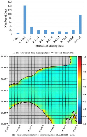
Figure 1.
The temporal and spatial distributions of missing rates of AVHRR SST data in the region of East China Sea in 2021.
A variety of methods have been proposed for satellite data imputation, and these methods can be roughly classified into three categories, i.e., statistical methods, traditional machine learning-based methods and deep learning methods. Statistical methods learn the linear or non-linear correlations in satellite data based on prior knowledge to achieve data imputation. Typical statistical methods include Optimal Interpolation (OI) method, Data Interpolation Empirical Orthogonal Function (DINEOF) method and distance-based method (e.g., Kriging and IDW). The OI method derives the optimal unbiased estimate of missing satellite data based on the min-variance and is often used to produce cloud-free products of SST data by fusing data from multiple platforms, e.g., satellite data, buoy data, and in situ data. For example, OI method is used in the OISST product from National Oceanic and Atmospheric Administration (NOAA) [12], Operational Sea Surface Temperature and Sea Ice Analysis (OSTIA) system [13], and blended foundation SST product [14]. OI method is also used for analyzing daily SST by fusing the AVHRR satellite data and Tropical Rainfall Measuring Mission Microwave Imager (TMI) product [15]. The DINEOF method achieves missing value imputation in oceanographic data [16] based on the Empirical Orthogonal Function (EOF). It is widely used for the reconstruction of Chl-a data [17,18,19], SST data [19,20], ocean wind data [21] and multivariate reconstruction [22]. The distance-based data imputation method achieves data imputation based on the spatial relevance of satellite data. Representative approaches include Kriging [23,24] and IDW [25]. Statistical methods have been widely used for filling missing values in various satellite data products. However, with the increasing of satellite data, it is time-consuming for statistical methods to construct correlation equations in satellite data. In addition, they cannot well learn the complex nonlinear relationships in satellite data to further improve the accuracy of data imputation.
Representative traditional machine learning methods for satellite data imputation include Random Forest (RF), eXtreme Gradient Boosting (XGBoost), k-Nearest Neighbors (KNN), Support Vector Regression (SVR) and Matrix Factorization (MF). The RF method and XGBoost method are typical tree-based ensemble methods [26], and fill missing values in satellite data by constructing multiple decision trees. Mohebzadeh et al. [27] compared RF method with DINEOR method for the imputation of Chl-a data from the MODIS satellite. Chen et al. [28] used RF to improve the coverage of Chl-a data with two external factors, i.e., the Ocean Color Index and the Rayleigh-corrected Reflectivity. In addition, RF and XGBoost are also used for the reconstruction of Chl-a satellite data [29,30,31,32]. The KNN method and SVR method fill missing data based on distance measurement, and have been widely applied for satellite data imputation [29,30,33,34]. Hankel Matrix Factorization (HMF) is used for data imputation in the Global Navigation Satellite System (GNSS) [35]. In practice, the traditional machine learning methods described above has some limitations for missing value imputation in satellite data. First, it is hard for them to fully mine the hidden information in the long time series satellite data. Second, the short-term temporal dependence and dynamic spatial dependence are also not well considered by these methods.
Deep learning methods can effectively learn the hidden regularity in satellite data [36,37], thus being introduced for satellite data imputation. Jean-Marie et al. [38] achieved the interpolation of SST data using a neural network, and proved that neural network is superior to the OI and EOF methods. Artificial Neural Network (ANN) has been also applied for the reconstruction of satellite data [30,33,39]. Jouini et al. [40] applied Self-Organizing Map (SOM) network to reconstruct Chl-a data by integrating SST and sea surface height (SSH). Data-Interpolating Convolutional Auto-Encoder (DINCAE) method is proposed for filling the missing values in SST data [41]. The Auto-Encoder in DINCAE is similar to the EOF for data reduction, and can effectively capture non-linear information of satellite data. DINCAE has been widely used for the reconstruction of Chl-a data [42] and SST data [43].
However, existing satellite data imputation methods still face some big challenges. First, the spatial dependence in satellite data is dynamic and affected by various uncontrollable factors around the target regions. For example, SST is usually affected by wind and solar radiation, and Chl-a concentration is vulnerable to the reproduction direction of phytoplankton. Second, satellite data usually show bidirectional short-term temporal dependence, and has large fluctuations in short term. For satellite data imputation, in addition to historical data, future data should be also taken into account because it is already known. For example, the occurrence of red tides causes the Chl-a concentration to be higher than usual. In this case, the imputation of missing values in Chl-a concentration is highly dependent on future data. Therefore, the bidirectional short-term temporal dependence should be fully utilized to improve the performance of satellite data imputation. Unfortunately, existing satellite data imputation methods cannot well learn the dynamic spatio-temporal dependence in satellite data to achieve accurate data imputation.
Therefore, in this work, we propose the Spatio-Temporal Attention Generative Adversarial Network (STA-GAN), which integrates Graph Attention Network (GAT) and Generative Adversarial Network (GAN) for missing value imputation in satellite data. GAN can efficiently learn the complex distribution of the data so that the generated data well conform to the original data distribution, and is suitable for time series data imputation [44]. Therefore, multiple GAN models, e.g., Generative Adversarial Imputation Network (GAIN) [45], GAN-2-stage [46] and SolarGAN [47]), have been introduced for missing data imputation. Meanwhile, the attention mechanism [48,49] can achieve dynamic aggregation of effective information and is widely used for the prediction of SST and Chl-a concentration [50,51,52]. Inspired by the attention mechanism, the GAT network processes graph nodes of different degrees and gives higher weights to the influential neighbor nodes [53]. GAT is suitable for mining the spatio-temporal dependence of ocean remote sensing data.
Concretely, STA-GAN first learns the short-term temporal dependence and dynamic spatial dependence with a Spatio-Temporal Attention mechanism based on GAT, and introduces GAN to learn the underlying distribution of satellite data. Then, we train the generator and discriminator of STA-GAN by fusing the learned spatio-temporal dependence features. Finally, the missing data is filled with the generated data by STA-GAN.
In sum, our contributions are summarized as follows:
- We identified the challenges in satellite data imputation and proposed the STA-GAN model that integrates GAT and GAN to achieve accurate data imputation.
- We developed a new spatio-temporal attention mechanism based on GAT to capture the short-term temporal dependence and dynamic spatial dependence of satellite data in parallel.
- We re-designed the structure of GAN to achieve data imputation by learning the distribution of satellite data with the learned spatio-temporal dependence information.
In addition, we evaluated STA-GAN model on both SST satellite data and Chl-a satellite data. The results demonstrate that STA-GAN outperforms a variety of existing data imputation methods, especially for filling satellite data with high missing rates.
The rest of this article is organized as follows. Section 2 describes the data materials, the pre-processing and methods details of STA-GAN model for satellite data imputation. Then, we present the results in Section 3 and give the discussion in Section 4. Finally, we draw the conclusions in Section 5.
2. Materials and Methods
2.1. Study Area and Data
We use the satellite data for both SST and Chl-a as examples to study the problem of missing value imputation in satellite data. Satellite data are usually grid data partitioned according to the latitude and longitude, and the value of each grid is obtained by retrieving the satellite observation images from the sensors deployed on satellites.
The SST data are from the Advanced Very High-Resolution Radiometer (AVHRR) and collected twice, i.e., daytime and nighttime, one day. The spatial resolution is 4 km (1/24° × 1/24°) and the time range is from 2000 to 2021. We select two study areas, i.e., [121.00°E–122.00°E, 30.00°N–31.00°N] in the East China Sea (referred to as SST-EAST) and [109.00°E–110.00°E, 13.00°N–14.00°N] in the South China Sea (referred to as SST-SOUTH). For SST-EAST dataset, we remove the grid regions with missing rates larger than 95% since they lack enough ground-truth samples to validate the filled values. In addition, the land region is not taken into account. Finally, there are 368 grid regions in SST-EAST dataset and the overall missing rate is 8.43%. Similarly, there are 428 grid regions in the SST-SOUTH dataset after the filtering operation, and the overall missing rate is 11.72%. Figure 2 and Figure 3 illustrate the spatial distributions of SST-EAST and SST-SOUTH, respectively, on a selected day.
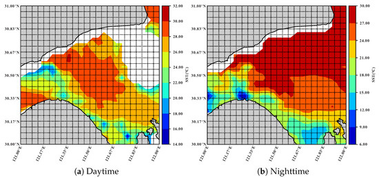
Figure 2.
The spatial distribution of SST-EAST dataset on Jul 18, 2021, where the white areas have no data, and the gray areas are land.
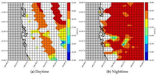
Figure 3.
The spatial distribution of SST-SOUTH dataset on Jul 17, 2021, where the white areas have no data, and the gray areas are land.
The Chl-a data is from the Ocean Color Climate Change Initiative 5.0 version (OC-CCI) product and collected once everyday. This product fuses the satellite data from SeaWiFS, MERIS, MODIS and VIIRS sensors to produce daily Chl-a data. The spatial resolution is also 4 km (1/24° × 1/24°) and the time range is from 2000 to 2021. The study area is [128.00°E–130.00°E, 24.00°N–26.00°N] in the East China Sea (referred to as CHA-EAST). The CHA-EAST dataset has 309 grid regions after removing the grid regions with missing rates larger than 95%, and its overall missing rate is 54.97%. Figure 4 shows the spatial distribution of CHA-EAST on 25 July 2021.
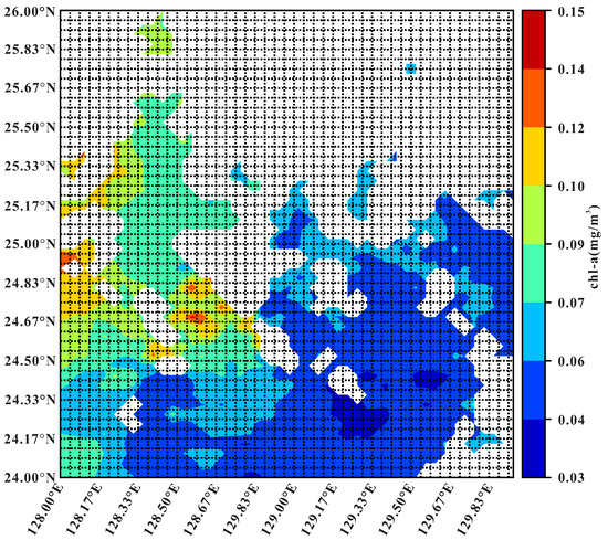
Figure 4.
The spatial distribution of CHA-EAST dataset on 25 July 2021, where the white areas have no data.
2.2. Data Processing
As illustrated in Figure 5, we use a dynamic graph to represent satellite data, where V is a set of N nodes and each node corresponds to a grid region; E is the set of edges and two nodes have an edge if their spatial distance is less than a given threshold. Given the locations and of nodes and , respectively, the distance between and is computed as below.
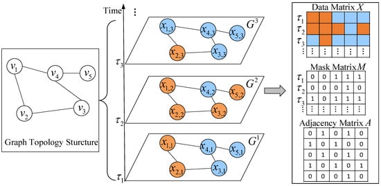
Figure 5.
The graph structure of satellite data, where orange color represents missing data, blue color represents observed data, and solid line indicates that two nodes are spatially connected.
We use an adjacency matrix to represent the topology structure of G. In matrix A, each entry indicates that there is an edge between nodes and , otherwise . The value of is determined as below.
where is a scaling factor, and is the threshold that controls the sparsity of matrix A. Two nodes are connected if their scaled distance is larger than or equal to the threshold . We also assume that the topology structure of graph G does not change over time, i.e., fixing matrix A.
As illustrated in Figure 5, for each timestamp , is used to represent the corresponding instant graph, which may contain missing values at some nodes. For example, in , nodes and have no values. For the whole graph G, we use matrix to record the time-series satellite data for N nodes at T timestamps, where is the observation values of satellite data for all nodes (i.e., grid regions) at timestamp , and is the observation value of node at timestamp . In addition, we introduce a masked matrix for X, where each entry if the entry is missing, otherwise
Given the incomplete satellite data matrix X and its masked matrix M, we aim to fill the missing values in X and ensure the filled values are close to the real values. To this end, we design the STA-GAN model to obtain an imputed matrix that is close to X, i.e.,
where is the generated matrix by STA-GAN model, is a matrix whose entries are all ones, and ⊙ denotes Hadamard product.
2.3. Methods
2.3.1. Overview
Figure 6 illustrates the structure of the STA-GAN model, which consists of spatio-temporal attention (STA) module and Generative Adversarial Network (GAN) module. First, STA learns the short-term temporal dependence and dynamic spatial dependence in satellite data based on GAT and produces the short-term temporal dependence representation matrix F and the dynamic spatial dependence representation matrix S. Then, the generator and discriminator of GAN are trained by fusing the learned spatio-temporal dependence features. Finally, the missing data is filled with the generated data by GAN module.
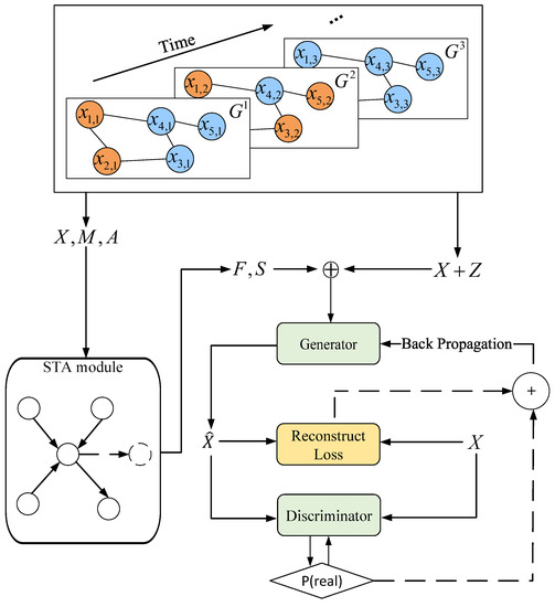
Figure 6.
The architecture of the STA-GAN model, where ⊕ denotes the concatenation operator, and + indicates the addition of two values.
2.3.2. Spatio-Temporal Attention for Dependence Learning
The STA consists of two operations, i.e., Temporal Attention (TA) operation and Spatial Attention (SA) operation, which are used to learn the short-term temporal dependence and dynamic spatial dependence, respectively.
- (a)
- Temporal Attention
The TA operation focuses on learning the short-term temporal dependence for the time series of each node in graph G. Concretely, we first divide into consecutive sub-sequences of the same length l, thus producing sub-sequences. For each node , we learn its short-term temporal dependence representation at timestamp as below.
where is the sigmoid activation function, represents the value of node at timestamp , is the set of timestamps that temporally affects node at timestamp , and is the normalized temporal dependence coefficient between timestamps and for node , i.e.,
where represents the temporal dependence coefficient between timestamps and for node , and is calculated by
where is a nonlinear activation function, ⊕ denotes the concatenation operator, is the learnable parameters of TA operation, and are the masked values of timestamps and , respectively, for node .
Figure 7 illustrates an example of TA operation. We set the length l to 3, and the first sub-sequence of node contains the values at timestamps , and . The corresponding values of at these three timestamps are , and , respectively. The value of node at timestamp is affected by values and with temporal dependence coefficient and , respectively. The short-term temporal dependence representation for node at time stamp is obtained by calculating .
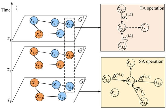
Figure 7.
Diagram of STA for temporal attention operation and spatial attention operation.
With temporal attention, we first calculate the short-term temporal dependence representation matrix for all nodes at each timestamp , i.e., , where represents matrix transpose. Then, we concatenate matrices to obtain the short-term temporal dependence representation matrix .
- (b)
- Spatial Attention
The SA operation learns the dynamic spatial dependence for each node in graph G. Concretely, for each node , we learn its dynamic spatial dependence representation at timestamp as below.
where is the sigmoid activation function, represents the value of node at timestamp , is the set of nodes that spatially affects node at timestamp , and is the normalized spatial dependence coefficient between nodes and at timestamp , i.e.,
where represents the spatial dependence coefficient between nodes and at timestamp and is calculated by
where is a nonlinear activation function, is the learnable parameter of SA operation, and and are the masked values of nodes and , respectively, at timestamp .
Figure 7 illustrates an example of SA operation. For timestamp , node is affected by nodes , and with spatial dependence coefficient , and , respectively. The dynamic spatial dependence representation for node at timestamp is obtained by calculating .
With spatial attention, we first obtain the dynamic spatial dependence representation matrix for all nodes at each timestamp , i.e., . Then, we combine to obtain the dynamic spatial dependence representation matrix .
2.3.3. Generative Adversarial Network for Data Imputation
GAN module achieves missing value imputation of satellite data by learning data distribution with the learned short-term temporal dependence matrix F and dynamic spatial dependence matrix S. We introduce Wasserstein GAN (WGAN) [54] to fill missing values in satellite data. In traditional WGAN, a pure noise matrix Z is usually used as the input of the generator to generate a matrix , where Z∼ is a pure noise matrix. This process does not consider the information about data, thus making it time-consuming to generate a matrix that is close to the real data distribution [47,55]. To address this issue, we integrate , the short-term temporal dependence representation matrix F and the dynamic spatial dependence representation matrix S as the inputs of the generator to provide comprehensive spatio-temporal dependence information for generating matrix . In addition, we re-design the structures of the generator and discriminator to enable them to handle the multiple inputs and to better learn the spatio-temporal distribution of satellite data. Figure 8 shows the structure of the generator of STA-GAN model that consists of a sequence of GRU units, and Figure 9 shows the structure of the GRU unit.
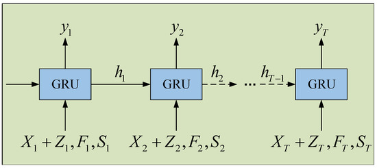
Figure 8.
The structure of the generator of STA-GAN model.
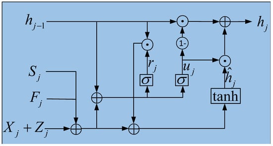
Figure 9.
The structure of GRU unit, where ⊙ is Hadamard product, and ⊕ is the concatenation operator.
The updating functions of GRU as listed as below.
where and are the update gates and reset gates, is the candidate hidden state, is the sigmod function, , , , and are the trainable parameters.
The discriminator has a similar structure to generator. The discriminator takes the original data matrix X and the generated matrix of the generator as inputs to obtain the probability of the authenticity of the generated matrix .
The loss function of the generator consists of reconstruction loss and the probability that the discriminator regards the generated matrix as the real data matrix, i.e.,
where is the hyper-parameter that balances reconstruction loss and the output probability . The reconstruction loss is the average absolute error between and X, i.e.,
The discriminator is designed to distinguish real data X and the generated matrix , and the loss function of the discriminator is
where and are the output probabilities of discriminator for matrices and X, respectively.
The back propagation method is used to optimize the loss function of the generator and discriminator by optimizing the corresponding parameters. Finally, we use the generated matrix to fill the missing values in the data matrix X, and obtain the imputation matrix .
3. Results
3.1. Experimental Settings
To evaluate the effectiveness and demonstrate the superiority of our STA-GAN model, we compare it with multiple baseline methods, including:
- (1)
- MEAN: achieves data imputation by using the mean values of historical records.
- (2)
- KNN [34]: finds the k nearest neighbors and fills in the missing value with the average of these neighbors.
- (3)
- GRU-D [56]: achieves the missing value imputation by introducing a decay mechanism in the input variable and hidden state to capture missing information.
- (4)
- GAIN [45]: a GAN-based data imputation method that introduces a hinting mechanism in discriminator to distinguish the original data and the generated data.
- (5)
- GAN-2-stage [46]: a data imputation method based on GAN through two-stage training. First, the decay mechanism is introduced into the generator and discriminator to consider time irregularity. Data imputation is then achieved based on the generated matrix from the trained GAN model.
- (6)
- SolarGAN [47]: an imputation method similar to GAN-2-stage that is used for solar data imputation. The difference with GAN-2-stage is that the noise matrix and the data matrix are fused as the inputs of the generator in SolarGAN.
Among these methods, GAIN, GAN-2-stage and SolarGAN are based on GAN and widely used for data imputation.
We use Mean Absolute Error (MAE) and Root Mean Square Error (RMSE) as performance evaluation metrics. For STA-GAN model, the length l of the divided sub-sequences is set to 12, and the learning rate is set to 0.001 for all methods. The batch sizes on SST-EAST, SST-SOUTH and CHA-EAST datasets are set to 64, 64 and 32, respectively. For all the experiments, the partition ratio of training, validation and testing data in each data set is set to 8:1:1. We use the Adam optimizer to update the parameters of model. All the data imputation models are implemented on TensorFlow 1.7.1. The dimension of pure noise matrix Z and GRU hidden state are both 64. In addition, we use a 64-core Intel Xeon processor with 256 GB RAM and 3 NVIDIA RTX 2080Ti GPUs.
3.2. Hyper-Parameter Selection
The adjacency matrix A is a representation of the neighbor nodes for each node. For each node, selecting a small number of neighbor nodes cannot fully cover all the spatial dependence information while selecting a large number of neighbor nodes may cause information bias and result in errors in the learned spatial dependence information. According to Equation (2), parameters and are used to control the number of neighbor nodes for each node. We thus conduct experiments on three datasets, respectively, to identify a good setting for the two parameters. Figure 10 presents the results of STA-GAN model while varying and , where the missing rate is 0.5. To generate data with different missing rates, we randomly mask some real data values in satellite data. According to the results, we set , for the SST-EAST and CHA-EAST datasets, and set , for the SST-SOUTH dataset.
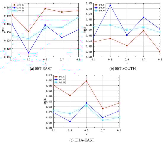
Figure 10.
The RMSE of STA-GAN model while varying and , where the missing rate is 0.5.
The parameter is used to balance the importance of reconstruction loss and the output probability of discriminator in STA-GAN model. Figure 11 illustrates the results of STA-GAN while varying , where the missing rate is 0.5. According to the results, we set = 200 for SST-EAST and SST-SOUTH datasets and = 300 for CHA-EAST dataset.
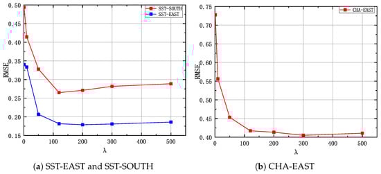
Figure 11.
The RMSE of STA-GAN model while varying , where the missing rate is 0.5.
3.3. Performance Comparison with Baseline Methods
Figure 12, Figure 13 and Figure 14 show the results of STA-GAN model and six baseline methods on the SST-EAST, SST-SOUTH, and CHA-EAST datasets, respectively, while varying the missing rate. Meanwhile, Table 1, Table 2 and Table 3 show the corresponding quantitative experimental results. In general, with the increase of the missing rate, the performance of all the data imputation methods, except for MEAN method, degrades. However, the performance decline trend of the STA-GAN model is significantly lower than that of other baseline methods, which indicates that STA-GAN effectively learns the spatio-temporal information in satellite data. Among the baseline methods, MEAN and KNN have the worst performance since they do not consider the correlations between time series. Meanwhile, GAN-2-stage, GRU-D and SolarGAN perform better than the other baseline methods. However, STA-GAN model outperforms all these baseline methods at various missing rates and the superiority increases rapidly when the missing rate increases. The reason is that STA-GAN provides enriched spatio-temporal information for data imputation (especially at high missing rates) by simultaneously learning the short-term temporal dependence and dynamic spatial dependence features.
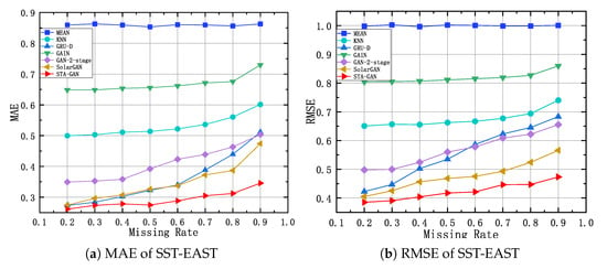
Figure 12.
MAE and RMSE of SST-EAST dataset with different missing rates.
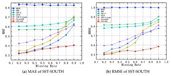
Figure 13.
MAE and RMSE of SST-SOUTH dataset with different missing rates.
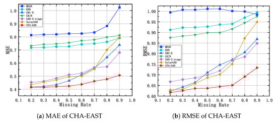
Figure 14.
MAE and RMSE of CHA-EAST dataset with different missing rates.

Table 1.
The results (RMSE and MAE) of SST-EAST dataset with different missing rates.
Table 2.
The results (RMSE and MAE) of SST-SOUTH dataset with different missing rates.
Table 3.
The results (RMSE and MAE) of CHA-EAST dataset with different missing rates.
3.4. Ablation Experiment
Table 4 shows the results of an ablation experiment for the STA-GAN model on three datasets, where the data missing rate is set to 0.5. According to the results, the performance of the STA-GAN model degenerates after removing the spatial attention and temporal attention, which validates the effectiveness of each module, and indicates that considering the spatio-temporal dependence in satellite data can help reduce the data imputation error.
Table 4.
The results of the ablation experiment.
4. Discussion
STA-GAN model is tailored for filling missing values in saptio-temporal data (e.g., SST satellite data and Chl-a satellite data) with high missing rates. To this end, it tries to learn comprehensive spatio-temporal dependence information from original data by combining Spatio-Temporal Attention and Generative Adversarial Network.
Figure 15 plots the original satellite data and the generated data by STA-GAN model while setting the missing rate to 0.2, 0.5 and 0.9, respectively. Three cases are from the CHA-EAST dataset and select one location without missing data in 2021. In all three cases, the imputed data has the similar trend with the original data, and the difference between the imputed data and the original data is small, especially at the missing rates of 0.2 and 0.5. For the data imputation at missing rate of 0.9, the error is large since quite limited knowledge can be learned from the real satellite data to support accurate data imputation.
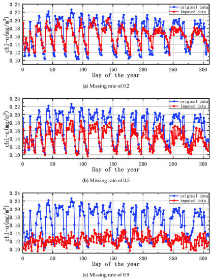
Figure 15.
The plotting of the original satellite data and the generated data by STA-GAN model with different missing rates.
According to the results in Section 3.3, compared with existing data imputation methods, STA-GAN model still has good data imputation performance under the high data missing rates, which is mainly due to the abundant spatio-temporal dependence information extracted by the model. On the one hand, the STA-GAN model considers the dynamic spatial dependence. The spatial dependence is dynamic over time. For example, the change of wind direction could result in the change of spatial dependence of SST, and the direction of red tide reproduction also affects the spatial dependence of chlorophyll concentration. Therefore, extracting dynamic spatial dependence information can effectively improve the data imputation performance. On the other hand, the bidirectional short-term temporal dependence is considered in STA-GAN model. In general, the missing data is usually similar to the data from the past few days, which is why existing data imputation models such as GRU-D [56], GAN-2-stage [46] and SolarGAN [47] consider historical data in the process of data imputation. However, for satellite remote sensing data, only considering the impacts of historical data is not enough since the missing data is also related to the patterns of future data. Therefore, considering the dynamic bidirectional short-term temporal dependence in STA-GAN model can better capture the dynamic changes of satellite data over time, thus bringing better data imputation performance.
5. Conclusions
In this article, we proposed the STA-GAN model for missing value imputation in satellite data. STA-GAN can effectively learn features for capturing both short-term temporal dependence and dynamic spatial dependence in satellite data and exploit the learned features to train a generative model to fill the missing values. According to the experimental results on three real datasets, STA-GAN model achieves much better performance than existing methods, especially for filling satellite data with large missing rates. For future work, we would like to consider some external factors, e.g., humidity and wind, to further enhance the performance of STA-GAN model.
Author Contributions
Conceptualization, S.W. and W.L.; data curation, S.W. and J.Y.; formal analysis, S.W. and W.L.; methodology, S.W., W.L. and S.H.; supervision, J.G.; validation, S.W.; visualization, S.W.; writing—original draft, S.W. and J.Y.; writing—review and editing, S.W. and W.L. All authors have read and agreed to the published version of the manuscript.
Funding
This work was supported in part by National Natural Science Foundation of China (No. 62202336, No. U1936205, No. 62172300), Shanghai Pujiang Program (No. 20PJ1414300), National Key R&D Program of China (No. 2021YFC3300300), Open Research Projects of Zhejiang Lab (No. 2021KH0AB04), and the Fundamental Research Funds for the Central Universities (No. ZD-21-202101).
Data Availability Statement
The SST satellite data provided by AVHRR is available from https://www.ncei.noaa.gov/, accessed on 11 October 2022. The Chl-a satellite data from OC-CCI products is available at https://www.oceancolour.org/, accessed on 11 October 2022.
Conflicts of Interest
The authors declare no conflict of interest.
References
- Martin, S. An Introduction to Ocean Remote Sensing; Cambridge University Press: Cambridge, UK, 2014. [Google Scholar]
- He, X.; Shi, S.; Geng, X.; Xu, L.; Zhang, X. Spatial-temporal attention network for multistep-ahead forecasting of chlorophyll. Appl. Intell. 2021, 51, 4381–4393. [Google Scholar] [CrossRef]
- Lee, M.S.; Park, K.A.; Chae, J.; Park, J.E.; Lee, J.S.; Lee, J.H. Red tide detection using deep learning and high-spatial resolution optical satellite imagery. Int. J. Remote Sens. 2020, 41, 5838–5860. [Google Scholar] [CrossRef]
- Qin, M.; Li, Z.; Du, Z. Red tide time series forecasting by combining ARIMA and deep belief network. Knowl.-Based Syst. 2017, 125, 39–52. [Google Scholar] [CrossRef]
- Zheng, G.; Li, X.; Zhang, R.; Liu, B. Purely satellite data–driven deep learning forecast of complicated tropical instability waves. Sci. Adv. 2020, 6, 1–9. [Google Scholar] [CrossRef] [PubMed]
- Woodring, J.; Petersen, M.; Schmeisser, A.; Patchett, J.; Ahrens, J.; Hagen, H. In Situ Eddy Analysis in a High-Resolution Ocean Climate Model. IEEE Trans. Vis. Comput. Graph. 2016, 22, 857–866. [Google Scholar] [CrossRef]
- Reichstein, M.; Camps-Valls, G.; Stevens, B.; Jung, M.; Denzler, J.; Carvalhais, N. Deep learning and process understanding for data-driven Earth system science. Nature 2019, 566, 195–204. [Google Scholar] [CrossRef]
- Gao, S.; Zhao, P.; Pan, B.; Li, Y.; Zhou, M. A nowcasting model for the prediction of typhoon tracks based on a long short term memory neural network. Acta Oceanolog. Sin. 2018, 37, 8–12. [Google Scholar] [CrossRef]
- Rüttgers, M.; Lee, S.; Jeon, S.; Donghyun, Y. Prediction of a typhoon track using a generative adversarial network and satellite images. Sci. Rep. 2019, 9, 6057. [Google Scholar] [CrossRef]
- Guan, L.; Kawamura, H. SST availabilities of satellite infrared and microwave measurements. J. Oceanogr. 2003, 59, 201–209. [Google Scholar] [CrossRef]
- King, M.D.; Platnick, S.; Menzel, W.P.; Ackerman, S.A.; Hubanks, P.A. Spatial and temporal distribution of clouds observed by MODIS onboard the terra and aqua satellites. IEEE Trans. Geosci. Remote Sens. 2013, 51, 3826–3852. [Google Scholar] [CrossRef]
- Huang, B.Y.; Liu, C.Y.; Banzon, V.; Freeman, E.; Graham, G.; Hankins, B.; Smith, T.; Zhang, H.M. Improvements of the Daily Optimum Interpolation Sea Surface Temperature (DOISST) Version 2.1. J. Clim. 2021, 34, 2923–2939. [Google Scholar] [CrossRef]
- Donlon, C.J.; Martin, M.; Stark, J.; Roberts-Jones, J.; Fiedler, E.; Wimmer, W. The operational sea surface temperature and sea ice snalysis (OSTIA) system. Remote Sens. Environ. 2012, 116, 140–158. [Google Scholar] [CrossRef]
- Kohtaro, H.; Futoki, S. Global daily high-resolution satellite-based foundation sea surface temperature dataset: Development and validation against two definitions of foundation SST. Remote Sens. 2016, 8, 962. [Google Scholar]
- He, R.; Weisberg, R.H.; Zhang, H.; Muller-Karger, F.E.; Helber, R.W. A cloud-free, satellite-derived, sea surface temperature analysis for the West Florida Shelf. Geophys. Res. Lett. 2003, 30, 1–5. [Google Scholar] [CrossRef]
- Beckers, J.; Rixen, M. EOF calculations and data filling from incomplete oceanographic datasets. J. Atmos. Ocean. Technol. 2003, 20, 1839–1856. [Google Scholar] [CrossRef]
- Liu, X.; Wang, M. Gap filling of missing data for VIIRS global ocean color products using the DINEOF method. IEEE Trans. Geosci. Remote Sens. 2018, 56, 4464–4476. [Google Scholar] [CrossRef]
- Guo, J.; Lu, J.; Zhang, Y.; Zhou, C.; Zhang, S.; Wang, D.; Lv, X. Variability of chlorophyll-a and secchi disk depth (1997–2019) in the Bohai Sea based on monthly cloud-free satellite data reconstructions. Remote Sens. 2022, 14, 639. [Google Scholar] [CrossRef]
- Ma, C.; Zhao, J.; Ai, B.; Sun, S. Two-Decade variability of sea surface temperature and chlorophyll-a in the Northern South China Sea as revealed by reconstructed cloud-free satellite sata. IEEE Trans. Geosci. Remote Sens. 2021, 59, 9033–9046. [Google Scholar] [CrossRef]
- Li, Y.; Sun, W.; Zhang, J.; Meng, J.; Zhao, Y. Reconstruction of arctic SST data and generation of multi-source satellite fusion products with high temporal and spatial resolutions. Remote Sens. Lett. 2021, 12, 695–703. [Google Scholar] [CrossRef]
- Zhao, X.; Hou, Y.; Qi, P. Interpretation of sea surface wind interannual vector EOFs over the China seas. Chin. J. Oceanol. Limn. 2010, 28, 340–343. [Google Scholar] [CrossRef]
- Alvera-Azcárate, A.; Barth, A.; Beckers, J.M.; Weisberg, R.H. Multivariate reconstruction of missing data in sea surface temperature, chlorophyll, and wind satellite fields. J. Geophys. Res.-Oceans 2007, 112, 1–11. [Google Scholar] [CrossRef]
- Bhattacharjee, S.; Mitra, P.; Ghosh, S.K. Spatial interpolation to predict missing attributes in GIS using semantic kriging. IEEE Trans. Geosci. Remote Sens. 2014, 52, 4771–4780. [Google Scholar] [CrossRef]
- Rossi, R.E.; Dungan, J.L.; Beck, L.R. Kriging in the shadows: Geostatistical interpolation for remote sensing. Remote Sens. Environ. 1994, 49, 32–40. [Google Scholar] [CrossRef]
- Lu, G.; Wong, D. An adaptive inverse-distance weighting spatial interpolation technique. Comput Geotech. 2008, 34, 1044–1055. [Google Scholar] [CrossRef]
- Shen, J.; Cao, J.; Liu, X.; Zhang, C. DMAD: Data-driven measuring of wi-fi access point deployment in urban spaces. ACM Trans. Intell. Syst. Technol. (TIST) 2017, 9, 1–29. [Google Scholar] [CrossRef]
- Park, J.; Kim, H.C.; Bae, D.; Jo, Y.H. Data reconstruction for remotely sensed chlorophyll-a concentration in the Ross Sea using ensemble-based machine learning. Remote Sens. 2020, 12, 1898. [Google Scholar] [CrossRef]
- Chen, S.; Hu, C.; Barnes, B.; Xie, Y.; Lin, G.; Qiu, Z. Improving ocean color data coverage through machine learning. IEEE T Geosci Remote. 2019, 222, 286–302. [Google Scholar] [CrossRef]
- Hu, C.; Feng, L.; Guan, Q. A machine learning approach to estimate surface chlorophyll a concentrations in global oceans from satellite measurements. IEEE Trans. Geosci. Remote Sens. 2021, 59, 4590–4607. [Google Scholar] [CrossRef]
- Mohebzadeh, H.; Mokari, E.; Daggupati, P.; Biswas, A. A machine learning approach for spatiotemporal imputation of MODIS chlorophyll-a. Int. J. Remote Sens. 2021, 42, 7381–7404. [Google Scholar] [CrossRef]
- Park, J.; Kim, J.H.; Kim, H.C.; Kim, B.K.; Bae, D.; Jo, Y.H.; Jo, N.; Lee, S.H. Reconstruction of ocean color data using machine learning techniques in Polar regions: Focusing on Off Cape Hallett, Ross Sea. Remote Sens. 2019, 11, 1366. [Google Scholar] [CrossRef]
- Xing, M.; Yao, F.; Zhang, J.; Meng, X.; Jiang, L.; Bao, Y. Data reconstruction of daily MODIS chlorophyll-a concentration and spatio-temporal variations in the Northwestern Pacific. Sci. Total Environ. 2022, 843, 156981. [Google Scholar] [CrossRef] [PubMed]
- Sunder, S.; Ramsankaran, R.; Ramakrishnan, B. Machine learning techniques for regional scale estimation of high-resolution cloud-free daily sea surface temperatures from MODIS data. Isprs J. Photogramm. 2020, 166, 228–240. [Google Scholar] [CrossRef]
- Poloczek, J.; Treiber, N.; Kramer, O. KNN Regression as Geo-Imputation Method for Spatio-Temporal Wind Data. In Proceedings of the International Joint Conference SOCO’14-CISIS’14-ICEUTE’14, Bilbao, Spain, 25–27 June 2014; Volume 299, pp. 185–193. [Google Scholar]
- Liu, H.; Li, L. Missing Data Imputation in GNSS Monitoring Time Series Using Temporal and Spatial Hankel Matrix Factorization. Remote Sens. 2022, 14, 1500. [Google Scholar] [CrossRef]
- Yuan, Q.; Shen, H.; Li, T.; Li, Z.; Li, S.; Jiang, Y.; Xu, H.; Tan, W.; Yang, Q.; Wang, J.; et al. Deep learning in environmental remote sensing: Achievements and challenges. Remote Sens. Environ. 2020, 241, 111716. [Google Scholar] [CrossRef]
- Wang, S.; Cao, J.; Yu, P. Deep learning for spatio-temporal data mining: A survey. IEEE Trans. Knowl. Data Eng. 2020, 34, 3681–3700. [Google Scholar] [CrossRef]
- Jean-Marie, V.; Frederic, J.; Ronan, F.; Baptiste, M.; Ludivine, L.; Christophe, D. Data-Driven interpolation of sea surface suspended concentrations derived from ocean colour remote sensing data. Remote Sens. 2021, 13, 3537. [Google Scholar]
- Pisoni, E.; Pastor, F.; Volta, M. Artificial neural networks to reconstruct incomplete satellite data: Application to the mediterranean sea surface temperature. Nonlinear Process Geophys. 2008, 15, 61–70. [Google Scholar] [CrossRef]
- Jouini, M.; Levy, M.; Crepon, M.; Thiria, S. Reconstruction of satellite chlorophyll images under heavy cloud coverage using a neural classification method. Remote Sens. Environ. 2013, 131, 232–246. [Google Scholar] [CrossRef]
- Barth, A.; Alvera-Azcarate, A.; Licer, M.; Beckers, J.M. DINCAE 1.0: A convolutional neural network with error estimates to reconstruct sea surface temperature satellite observations. Geosci. Model Dev. 2020, 13, 1609–1622. [Google Scholar] [CrossRef]
- Han, Z.; He, Y.; Liu, G.; Perrie, W. Application of DINCAE to reconstruct the gaps in chlorophyll-a satellite observations in the South china sea and West philippine sea. Remote Sens. 2020, 12, 4805. [Google Scholar] [CrossRef]
- Jung, S.; Yoo, C.; Im, J. High-Resolution seamless daily sea surface temperature based on satellite data fusion and machine learning over kuroshio extension. Remote Sens. 2022, 14, 575. [Google Scholar] [CrossRef]
- Kim, J.; Tae, D.; Seok, J. A survey of missing data imputation using generative adversarial networks. In Proceedings of the 2020 International Conference on Artificial Intelligence in Information and Communication (ICAIIC), Fukuoka, Japan, 19–21 February 2020; IEEE: Piscataway, NJ, USA, 2020; pp. 454–456. [Google Scholar]
- Yoon, J.; Jordon, J.; Schaar, M. GAIN: Missing Data Imputation using Generative Adversarial Nets. In Proceedings of the International Conference on Machine Learning, Stockholm, Sweden, 10–15 July 2018; pp. 1–10. [Google Scholar]
- Luo, Y.; Cai, X.; Zhang, Y.; Xu, J.; Yuan, X. Multivariate Time Series Imputation with Generative Adversarial Networks. In Proceedings of the Neural Information Processing Systems, Montreal, QC, Canada, 3–8 December 2018; pp. 1–12. [Google Scholar]
- Zhang, W.; Luo, Y.; Zhang, Y.; Srinivasan, D. SolarGAN: Multivariate solar data imputation using generative adversarial network. IEEE Trans. Sustain. Energy 2020, 12, 743–746. [Google Scholar] [CrossRef]
- Chorowski, J.K.; Bahdanau, D.; Serdyuk, D.; Cho, K.; Bengio, Y. Attention-based models for speech recognition. Adv. Neural Inf. Process. Syst. 2015, 28, 1–9. [Google Scholar]
- Vaswani, A.; Shazeer, N.; Parmar, N.; Uszkoreit, J.; Jones, L.; Gomez, A.N.; Kaiser, Ł.; Polosukhin, I. Attention is all you need. Adv. Neural Inf. Process. Syst. 2017, 30, 1–11. [Google Scholar]
- Xie, J.; Zhang, J.; Yu, J.; Xu, L. An adaptive scale sea surface temperature predicting method based on deep learning with attention mechanism. IEEE Geosci. Remote. Sens. Lett. 2019, 17, 740–744. [Google Scholar] [CrossRef]
- Guo, X.; He, J.; Wang, B.; Wu, J. Prediction of Sea Surface Temperature by Combining Interdimensional and Self-Attention with Neural Networks. Remote Sens. 2022, 14, 4737. [Google Scholar] [CrossRef]
- Wang, X.; Xu, L. Unsteady multi-element time series analysis and prediction based on spatial-temporal attention and error forecast fusion. Future Internet 2020, 12, 34. [Google Scholar] [CrossRef]
- Veličković, P.; Cucurull, G.; Casanova, A.; Romero, A.; Lio, P.; Bengio, Y. Graph attention networks. arXiv 2017, arXiv:1710.10903. [Google Scholar]
- Arjovsky, M.; Chintala, S.; Bottou, L. Wasserstein generative adversarial networks. In Proceedings of the International Conference on Machine Learning, Sydney, Australia, 6–11 August 2017; Volume 70, pp. 214–223. [Google Scholar]
- Wang, S.; Cao, J.; Chen, H.; Peng, H.; Huang, Z. SeqST-GAN: Seq2Seq generative adversarial nets for multi-step urban crowd flow prediction. ACM Trans. Spat. Algorithms Syst. (TSAS) 2020, 6, 1–24. [Google Scholar] [CrossRef]
- Che, Z.; Sanjay, P.; Kyunghyun, C.; David, S.; Liu, Y. Recurrent Neural Networks for Multivariate Time Series with Missing Values. arXiv 2016, arXiv:1606.01865. [Google Scholar] [CrossRef]


Disclaimer/Publisher’s Note: The statements, opinions and data contained in all publications are solely those of the individual author(s) and contributor(s) and not of MDPI and/or the editor(s). MDPI and/or the editor(s) disclaim responsibility for any injury to people or property resulting from any ideas, methods, instructions or products referred to in the content. |
© 2022 by the authors. Licensee MDPI, Basel, Switzerland. This article is an open access article distributed under the terms and conditions of the Creative Commons Attribution (CC BY) license (https://creativecommons.org/licenses/by/4.0/).