Abstract
For the mosaicking of multiple remote sensing images, obtaining the optimal stitching line in the overlapping region is a key step in creating a seamless mosaic image. However, for very large remote sensing images, the computation of finding seamlines involves a huge amount of image pixels. To handle this issue, we propose a stepwise strategy to obtain pixel-level optimal stitching lines for large remote sensing images via an upscaling–downscaling image sampling procedure. First, the resolution of the image is reduced and the graph cut algorithm is applied to find an energy-optimal seamline in the reduced image. Then, a stripe along the preliminary seamline is identified from the overlap area to remove the other inefficient nodes. Finally, the graph cut algorithm is applied nested within the identified stripe to seek the pixel-level optimal seamline of the original image. Compared to the existing algorithms, the proposed method produces fewer spectral differences between stitching lines and less-crossed features in the experiments. For a wide range of remote sensing images involving large data, the new method uses less than 10 percent of the time needed by the SLIC+ graph cut method.
1. Introduction
It is increasingly convenient to acquire and use big data remote sensing images thanks to the accelerated development of sensor manufacturing technology. Over the past decade, remote sensing imagery has been used extensively in disaster avoidance, flood surveillance, shoreline protection, and urban planning. However, the restricted geographical range is one of the major limitations to its wider application. Generally, a solitary image cannot reach a vast area for investigation since its dimension is limited, which means that the region of interest (ROI) cannot be fully contained in a single image. Image mosaicking is the procedure of combining two or more images with overlapped areas into a single view with indistinguishable seamlines [1]. Various algorithms have been developed for such image mosaicking. These existing algorithms can be broadly classified into two categories: To find the minimum color difference between the two sides of the seamline [2,3,4,5,6] and to find the minimum number of features to be crossed by the mosaicking procedure [7,8,9,10]. The former exploits image color information to guide the seamline, avoiding seamlines through areas with large color contrasts and ensuring that color differences along the seamline are minimized. In the latter case, the image is divided into features or applied auxiliary data before guiding the seamline, so that the seamline avoids prominent feature areas of the image to ensure that the seamline crosses a minimum number of features.
For color-difference-minimum algorithms, this type of method usually considers only the color information of the image, simply inputting the original image and applying its color information to determine the seamline with the least overlapped areas. Typically, these methods can acquire the optimal seamline with minimum cost of computing by building a cost function to represent the difference between image metric points. Kerschner et al. [11] presented the double snake algorithm, though it is mainly applicable to forested areas and results in a locally optimal rather than globally optimal solution. With the help of Dijkstra’s algorithm [12], Chon et al. [13] used normalized cross-correlation as a cost to minimize the discrepancy level into the suture, but the method requires to assign the starting and ending points. Ma and Sun [14] developed a novel A* algorithm [15] to obtain the global optimal splicing line by optimizing the improved A* algorithm. Yu et al. [16] obtained the information of color, edge, and texture to capture the similarity of the images. All these metric values are then employed as input to the cost function to guide the seamline through a dynamic programming algorithm. Meanwhile, many scholars have applied the spatial ant colony algorithm [17,18] in the method of obtaining the optimal seamline. Recently, Wang et al. [19] proposed to generate a cost function (initial pheromone) in terms of gray difference and gray gradient while iteratively implementing a continuous space ant colony algorithm to pick the minimum cost path for the optimal embedded stitch. However, their method does not accommodate the mosaic suture vertices of the non-sequential alignment. In comparison, this method requires only two original datasets, which is not highly dependent on the data and is widely applicable; however, it cannot guarantee to avoid the distortion of some feature information in the mosaic image received from the mosaic.
For objects-through-minimum algorithms, the aim is to avoid traversing the majority of visually obvious objects with the seamline, so that the mosaic image retains the most complete feature information. This kind of approach normally requires a semantic segmentation procedure or the application of auxiliary data to segment the features. First, based on the semantic segmentation approach, the segmentation results are used to calculate the energy cost. Taking an example of Soille [20], in which an image synthesis algorithm was developed based on mathematical morphology and its label-controlled segmentation paradigm, which seeks suture lines along important image structural frames to cut down the number of segmented features within the output mosaic image. Pan et al. [21] described a method to determine the seamline for an orthophoto mosaic using the region change rate (RCR). The method utilizes the mean shift segmentation algorithm to segment the overlapping area, and then inspects the change index of the segmented regions; it classifies the overlapping area into three layers: preferred regions, general regions and obstacle regions. Li et al. [22,23] and Yuan et al. [24] introduced super-pixel segmentation to segment the overlapping region of the initial image into different feature regions, thus applying the graph cut algorithm to gain the optimal seamline. However, semantic segmentation without auxiliary data implies the need for well-developed semantic segmentation algorithms and great algorithmic efficiency allocated to the process of semantic segmentation. Yang et al. [25] proposed to triangulate the overlapping region into a mesh, thus assembling the original pixels into a series of triangle; this can better combine auxiliary methods or other data. On the other hand, many methods are based on auxiliary data. With the help of digital elevation model (DEM) data, Chen et al. [26] applied their own method to urban area seamline detection; but DEM data is the outcome of the digital surface model (DSM) data filtering and the filtering process still requires more enhancement, as high-quality DEM data is extremely rare. Some scholars [27,28] used DSM data directly, thus adjusting the vertices of the image seams so that they avoid crossing the building. Wan et al. [29] introduced road vector data so that the joint line can perfectly avoid crossing roads. Similarly, Wang et al. [30] introduced building vector data so that the joint line can avoid crossing buildings. Meanwhile, Zheng et al. [31] used DSM data to extract edge maps so that the vertices can be relocated to obtain an optimized seamline. Those auxiliary data can indeed help achieve the required reduction in the number of features crossed by the splicing line, but this category of method requires complete auxiliary data and the splicing results are highly correlated with the auxiliary data. The quality of the auxiliary data directly impacts the quality of the splicing results.
A great deal of algorithms have been proposed to minimize the color difference of the mosaic or to reduce the number of features traversed by the seamline. Yet, for large-scale remote sensing images, which have a greater abundance of geographic information and consequently larger data volume, the application of the above-mentioned algorithms mostly leads to low efficiency. The result is a massively time-consuming seamline finding process and even algorithm failure. We aim to solve this problem and achieve fast, efficient and superior results even when facing the mosaicking process of remote sensing images of very large files. Thus, our new method can compensate the “failure” of existing methods for the mosaicking process of ultra-large remote sensing images. In this paper, we formulate an upscaling–downscaling strategy for ultra-large remote sensing images. To achieve the optimal seamline more efficiently, we utilize the nested seamline acquisition scheme. First, the original image is reduced, which can significantly cut down the number of pixel nodes by building an undirected graph, applying the graph cut algorithm [32,33] to obtain a sub-optimal splicing line. We establish a new search domain on the raw image depending on the first acquired seamline. This allows us to eliminate most of the "inefficient" nodes so that during the second capture of the seamline, all nodes are efficient. Then, in the search field we perform the second undirected graph creation and the application of the graph cut algorithm to obtain the pixel-level optimal seamline.
2. Methodology
Figure 1 shows the proposed mosaic algorithm for very large remote sensing images. Note that in this paper, we consider only a mosaic of two images, which can be arbitrarily positioned relative to each other. The algorithm involves three steps. First, the raw image is reduced to find a rough seamline. Second, a buffer is created according to this seamline to generate a band of overlapping regions on the original images, and the graph cut algorithm is applied again in this ribbon area to perform a more refined pixel-level optimal seamline search of the original images. Finally, we apply color leveling and mosaic treatment according to this optimal seamline. These are described in detail below.
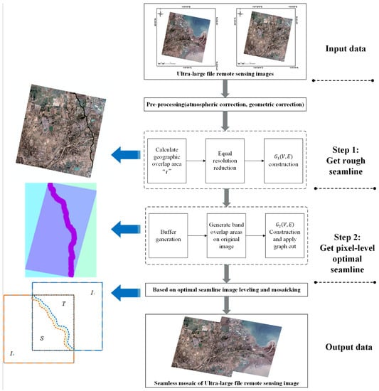
Figure 1.
Flowchart of the proposed high-performance mosaic optimization algorithm for very large remote sensing images.
Moreover, image elements are utilized for bridging graph nodes and their corresponding image regions in the graph cut algorithm formula. The image element is represented as an image pixel when the graph cut algorithm is applied in the original image. It also stands for pixels in the resampling region, or one segment in the segmentation result, when the graph cut algorithm is fulfilled in the reduced image or the segmented image, respectively.
2.1. Pre-Processing
It is important to obtain the exact grayscale value of each image and to remove the geometric distortion of the image for the subsequent process. Therefore, radiometric correction and geometric correction are indispensable in pre-processing to gain optimal seamlines. One can eliminate the influence of atmospheric and lighting factors on the reflection of the ground, so as to obtain more realistic inversion of the true reflectance of the ground; the other is able to cancel geometric distortion of the image with respect to the ground target caused by factors such as the satellite attitude, altitude, and speed, and rotation of the Earth. For the radiometric correction, we recover the image radiance first through the extremely accessible sensor calibration parameters “gain and offset,” and then normalize it using the FLAASH atmospheric physics model [34]. In the geometric correction process, we use ground control points and a geometric correction mathematical model to perform the correction of errors generated by non-systematic factors. In addition, the remote sensing image software is used to perform image registration processing on the images before mosaicking. This pre-processing lays the foundation for a more seamless follow-up and makes our approach more general.
2.2. Obtain a Rough Seamline
2.2.1. Image Reduction
To obtain a rough seamline more efficiently, we utilize down-sampling to shrink the original images; in this way, we greatly reduce the computational effort while finding the seamline for the first time. First, to guarantee that the number of image elements after down-sampling satisfies the number of nodes required by the graph cut algorithm for large-scale remote sensing images, the number of image elements in the overlapping domain needs to be counted and the resampling resolution. In this study, we found that the number of overlapping area elements and the initial stitching lines obtained after down-sampling are superior when the resampling factor is selected. At the same time, to assure efficiency while taking into account the accuracy of the final image, we use the bilinear interpolation [35] method for image reduction, which provides a compromise between computational efficiency and image quality.
2.2.2. Establishing Network Flow
The establishment of the network flow is critical for seeking the seamline and the eventual mosaic. In order to greatly reduce the parallax of the mosaicked image and create the appearance of a seamless mosaic, we need to obtain minimal spectral differences. In this paper, an undirected graph with information on the correct values of each edge is created based on the overlapping regions. contains the graph node and the edge , where stands for the average of the spectral values of multiple bands at node . denotes the edges between internal nodes and denotes the outermost edge of the graph frame for the graph cut algorithm. The edges between internal nodes and the edges on the frame are given different assignments so that the seamline avoids the edges at the very edges of the frame. The assignment rules for each node and edge in the undirected graph are given follows:
The value of the node is the average spectral value of the corresponding image element, which stands for the reduced pixels in the resampling region, or one pixel in the original image.
The edges between internal elements:
where denotes the edge from the element to element . corresponds to the mean spectral value for image element at image p, is the mean spectral value for corresponding image element at image q. And similarly, denotes for image element at image p and denotes for image element y at image q, respectively.
The outermost edge of the frame:
where denotes the edge between image element and image element at the outermost part of the frame. denotes the set of all . The purpose is to make the outermost edge of the frame the maximum value (Figure 2).
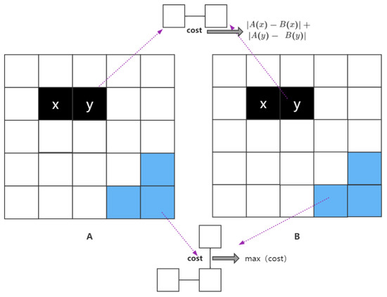
Figure 2.
Example diagram of network flow establishment. The black part uses the internal element assignment method, and the blue part uses the edge element assignment method.
2.2.3. Graph Cut
At this point, all edges in the undirected graph are assigned a non-negative weight . We call this cost. Then, the problem of searching for the optimal seamline can be combined with energy minimization problem of the graph cut algorithm. We can find the optimal suture line by the created undirected graph. An illustration of the graph-cut algorithm is presented in Figure 3. An energy-optimal seamline is obtained by extracting image element information from the overlapping regions the two images to form an undirected map with energy terms. The total energy cost consists of a data cost term and a smoothing cost term . that is:
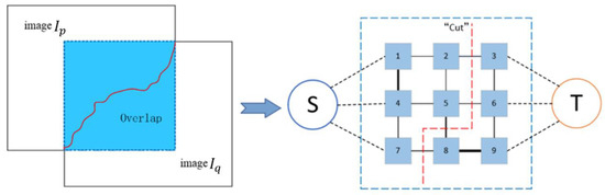
Figure 3.
Illustration of optimal seamline via graph cut. We denote each image element as a node and the energy cost between pixels as the weight of an edge. The “cut” marked next to the red dotted line denotes the min-cut.
The energy cost term refers to all costs per image element of the two input images p and q, that is,
In (5), p and q denote the two images, respectively. , n = p or q, denotes the sum of the energy costs of the labels assigned in the streaming network image , that is,
where x represents the image element belonging to and denotes x belonging to the energy cost contained in the label . If x , ; then, we define the energy cost as 0. Otherwise, if x, , then we define the energy cost as . According to the above definitions, the energy cost of each image element x in depends on whether it is within the effective area of an image or not.
When building an undirected graph, we assign weight between each resampling region, or one pixel point of the two images. The smoothing cost term for penalizing adjacent image element points is assigned as different labels. For two adjacent image elements x and y, where the smoothing cost term is defined as follows:
where denotes the cost of the edge connecting node x and node y. denotes the set of all neighboring node pairs in the 4-domain. denote the labels to which they belong. The function is a binary logic function; if , then = 0. Additionally, if , then = 1.
Now, all energy functions are converted to the functions available within the standard graph cutting framework of energy minimization [32]. Therefore, we can straightforwardly apply the graph cut algorithm to gain the optimal splice line in the overlapping domain. Applying the graph cut algorithm, we can partition the overlapping region into two zones (S and T). The line that divides it is called a “cut”, and if the energy that this line crosses is the smallest, then it is called a min-cut. In addition, when giving labels, we only consider the image elements that have values in the overlapping domain of both images, where the single image has value image element points can be directly set as the labels of its corresponding image.
Simultaneously, we consider that even if the resulting seamline is optimal, the upper and lower boundaries of the native images will cause significant parallax in the stitched image. When choosing the start and end points of the seamline, we need to consider the intersection of the overlapping region, so that the seamline goes from one corner vertex of the overlapping region to the other corner vertex. In this paper, our examples include the following location cases, which can be widely distributed over the relative location of different remote sensing images (Figure 4).
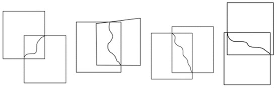
Figure 4.
Different location relations of remote sensing images of very large files.
2.3. Obtain the Pixel-Level Global Optimal Seamline
Obviously, the seamline obtained in the first step is not equal to the optimal seamline of the original image, so we need to nest again to gain the pixel-level optimal seamline with the help of the graph cut algorithm. Then, the second search for seamlines can be based on the seamline obtained in the first search. We use the buffer-building method to determine the range of the secondary search. The buffer radius can be determined based on the number of overlapping domain pixels calculated in step 2.2.1. Due to the need to balance efficiency and reliability, the buffer radius in this paper is generally chosen to be 17 image points. A band buffer range is obtained by buffering on the reduced image in the direction normal to the seamline to both sides; and then we map this band range to the original image one by one. We take into account that some of the buffer locations (at the head and tail of the stitching line) have image element points beyond the overlapping region of the original image. In this paper, after mapping the image to the original image, the corresponding search is performed to find points at the edges that do not belong to the overlapping region of the original image. Thus, a strip-like area with a radius of 170 pixels is formed on the original image, as shown in Figure 5. This strip area is the range where the final optimal splice line is found.
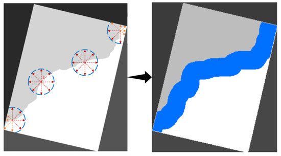
Figure 5.
Band overlapping region creation diagram.
Based on the image elements in the ribbon area, we can create the undirected graph , where each side is assigned in the same way as the side assignment rules given in Section 2.1. We apply the established undirected graph to the graph cut algorithm again to find the optimal seamline for the second time. At this point, the size of the image element is the size of the original image pixel. Then, when applying the graph cut algorithm, the image elements traversed by its computation process remove the relatively invalid elements deleted by the first seamline search, so the seamline obtained the second time is the optimal seamline at the pixel level.
2.4. Image Color Blending
In this article, we use a simple but effective method to even out the color. In the previous steps, we have divided the overlapping region into two pieces, S and T, which correspond to the original two images; S will complement the original image while T will complement the reference image. On both sides of the seamline, we select the image elements of the left and right sides, respectively, to form the set CP(Si), Cq(Si) and . denotes the i-th pixel in the set of the first pixel to the left of the seamline counting from top to bottom. i indicates the order. First, the adjustment factor for each band is calculated by the following equation:
where K denotes the total number of points in the set consisting of the first pixel to the left or right of the seamline. denotes the i-th pixel from top to bottom in the part of the image defined as S at a distance of 1 from the seamline. Likewise, denotes the i-th pixel from top to bottom in the part of the image defined as S at a distance of 1 from the seamline; denotes the i-th pixel from top to bottom in the part of the image defined as T at a distance of 1 from the seamline. It should be noted that indicates the adjustment factor of each band, so we will homogenize each band in turn to obtain each adjusted band and then perform multi-band fusion.
After obtaining the average color difference of each band, we obtain the image element value after mosaicking through the formula of color leveling (Figure 6). The formula of color leveling is as follows:
where denotes the value modified at pixel i in the final color leveling result. denotes the i-th pixel from the left to right in the part of the image , which is defined as T; denotes the i-th pixel from the left to right in the part of the image , which is defined as T. is the smoothing factor, which determines the final uniform color smoothness and the sense of chromatic aberration in the final image. If is too large, the image will show obvious color distortion; and if is too small, the image will show significant stitching color difference. The size of h is determined by the number of image elements in the actual experimental data set. In this paper, and are hyperparameters, we choose = 50, = 3.
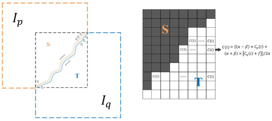
Figure 6.
Adjustment of the original image leveling process and the reference image pixel point value during the leveling process.
3. Experiments and Results
3.1. Experiment Scheme and Environment
To confirm the superiority of the method proposed in this paper, we selected four large remote sensing images (over 10 million pixels) with different data volumes. They contain a broad range of four types of satellite images (LandSat, Sentinel2-A, ZY-3 and GF-1) that are widely used today. They have different resolutions and numbers of pixels. Details are listed in Table 1. It is worth mentioning that, to demonstrate the effectiveness and advantage of our algorithm for very large files, we selected images with large data size.

Table 1.
Description of the data used in the experiments.
We tested six different methods using the above dataset. They consist of two combinations of graph cut, Dijkstra algorithm for finding seamlines, and super-pixel, down-sampling ideas for better efficient acquisition of optimal seamlines to form graph cut [22], Dijkstra [13], SLIC (simple linear iterative clustering) + graph cut [23], SLIC+ Dijkstra (the SLIC algorithm is applied to super-pixel division of the original image, and the Dijkstra algorithm is used to obtain the energy-optimal stitching line with each super-pixel as a node), resample + Dijkstra (application of Dijkstra’s algorithm to find the energy-optimal seamlines in the reduced image, and a buffer is created based on the first seamline to nest in the identified stripes. The pixel-level optimal seamline of the original image is sought again by the Dijkstra algorithm) and our proposed algorithm. For the reduced image, the down-sampling factor was set to 10, and the buffer radius was set to 17. For super-pixel division, the number of super-pixels was set to 25,000, and the super-pixel search step was set to 10. All of our experiments were conducted on a computer with AMD R7 5800H 3.20GHz CPU, 16GB RAM and 64bit Window 11 OS.
3.2. Results
Prior to creating the mosaic, the experimental data were pre-processed (step 2.1) to avoid as much as possible the errors caused by the images and the sensors themselves. All experimental data were atmospherically corrected and orthorectified before pre-processing.
3.2.1. Big Data Remote Sensing Images
We present the input images (Dataset 1 and Dataset 2) various seamlines, various stitching results, and their corresponding enlarged areas. Meanwhile, a schematic of the local results of super-pixels is shown.
For Dataset 1, we selected different resampling coefficients for the experiment in down-sampling and obtained the data results shown in Table 2. From the data in the table, we can see that when a sampling factor of 10 is selected, it has a shorter time consumption, the smallest color difference, and the least number of features traversed. So, it is obvious that it takes into account the three indicators and has the optimal results when the sampling factor is set to 10. However, for images of other data sizes we cannot guarantee that they will have optimal results when the sampling factor is set to 10. This requires a problem-specific analysis. In Table 2, average color difference represents the average of the difference in spectral values between the first points on either side of the seamline. Number of features crossed indicates the number of significant features crossed by the mosaic in the original image. The refined range interval means the set obtained by counting the cost on both sides of each pair of splice lines, where cost represents the average spectral difference of its pair of points (the first point on both sides of the splice line on the same row).
Table 2.
Results obtained by selecting different resampling factors for Dataset 1.
Dataset 1 and Dataset 2 are obtained with all six algorithms to obtain seamlines. From Dataset 1, our method can effectively produce a seamless mosaic image. Let us look specifically at the direction of the seamline. In the road area in the image (yellow box in Figure 7), our algorithm avoids crossing the road area multiple times; and the super-pixel (SLIC+ Dijkstra) algorithm crosses the road area multiple times. In the shoreline area of the image (blue box in Figure 7), the seamline in our algorithm travels along the shoreline, but there is still a section that crosses the coastal zone buildings (harbor platform), which is not as good as the algorithm that references super-pixels. From Dataset 2, our method is also effective in producing a seamlessly stitched image. In terms of the overall mosaic alignment, our approach yields a mosaic that avoids crossing dense areas of buildings and thus crosses fewer prominent features. In the area of buildings in the image (blue box in Figure 8), our algorithm has chosen to travel along urban roads and rivers as often as possible. It is true that in Dataset 1, the algorithm citing super-pixels outperforms our method in terms of the number of features traversed; however, in Dataset 2, our method instead traverses fewer features. This can also be seen from the super-pixel segmentation results in Figure 9. In Figure 9c,d, the super-pixels themselves also segment the features due to the large difference in size of the features in the image, thus not achieving the desired effect. Meanwhile, in the urban river area in the image (in the green box of Figure 8), the seamline obtained by our algorithm follows the river boundary.
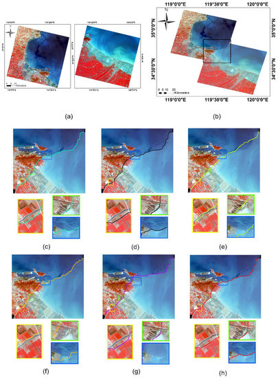
Figure 7.
Comparison of the seamlines on Dataset 1: (a) Original large remote sensing images. The stitching result obtained by (b) using our proposed method; (c) Dijkstra; (d) graph cut; (e) SLIC+ Dijkstra; (f) SLIC+ graph cut; (g) Resample+ Dijkstra; and (h) ours. Three locations are selected to show the refinement differences of the seamlines obtained by different algorithms with rectangular boxes of different colors. The colored line in the image is the seamline.
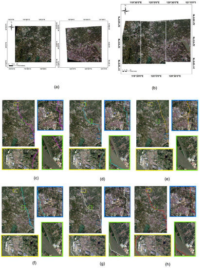
Figure 8.
Comparison of the seamlines of Dataset 2: (a) original large remote sensing images; the stitching result obtained by (b) our method; (c) Dijkstra; (d) graph cut; (e) SLIC+ Dijkstra; (f) SLIC+ graph cut; (g) resample+ Dijkstra; and (h) ours. Three locations are selected to show the refinement differences of the seamlines obtained by different algorithms with rectangular boxes of different colors. The colored line in the image is the seamline.
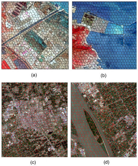
Figure 9.
Partial display of super pixel results. (a) Presentation of Dataset 1 super-pixel result of road and farmland. (b) Presentation of Dataset 1 super-pixel result of coastal zone display. (c) Presentation of Dataset 2 super-pixel result of the rivers in a city. (d) Presentation of Dataset 2 super-pixel result of the city’s buildings.
3.2.2. Ultra-Large Data Remote Sensing Images
We show the input image (Dataset 3 or Dataset 4) and the seamlines obtained by the algorithm that can find them. We also show their graphs with their corresponding enlarged areas.
Dataset 3 has only three algorithms to obtain the seamlines, while Dataset 4 has only two methods to obtain the seamline. Our method produces a seamlessly stitched image even in the presence of such a huge remote sensing image. Specifically, let us see the mosaic line orientation. From Dataset 3, in the area of farmland in the image (blue and green boxes in Figure 10), our approach extends as far as possible along the edges of the farmland blocks. In the area of the town in the figure (yellow box in Figure 10), the seamline achieved by our method stretches along the town road and river as it crosses the area. From Dataset 4, in the maritime building area of the image (yellow box in Figure 11) our approach avoids traveling along the edges of the buildings; in the offshore fishing boat area of the image (blue box in Figure 11), our approach also does a good job of avoiding dividing up the fishing boats.
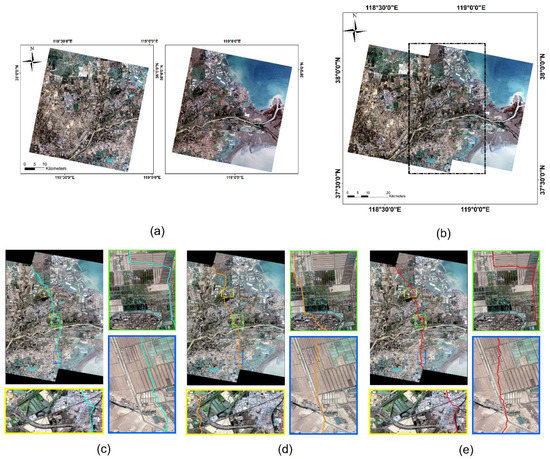
Figure 10.
Comparison of the seamline on Dataset 3: (a) original large remote sensing images; the stitching result obtained by (b) our method; (c) Dijkstra; (d) Resample+ Dijkstra; and (e) ours. Three locations are selected to show the refinement differences of the seamlines obtained by different algorithms with rectangular boxes of different colors. The colored line in the image is the seamline.
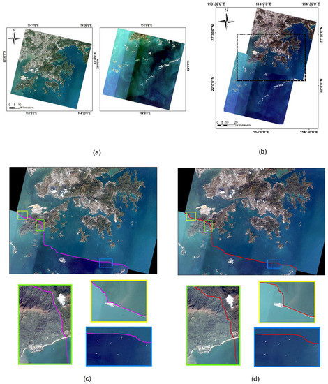
Figure 11.
Comparison of the seamlines on Dataset 4: (a) original large remote sensing images; the stitching result obtained by (b) our method; (c) Resample+ Dijkstra; and (d) ours. Three locations are selected to show the refinement differences of the seamlines obtained by different algorithms with rectangular boxes of different colors. The colored line in the image is seamlines.
In summary, visually our method produces a mosaic image without significant chromatic aberration in the face of a wide variety of remote sensing images with different relative positions and different data sizes. More importantly, there are no significant color cliff changes when looking at images of areas near the stitching line. Furthermore, the splicing line basically does not cross the significant feature area, which may cause the deformation of the feature caused by splicing.
4. Discussion
A performance comparison between five existing algorithms and the proposed method is listed in Table 3. For Dataset 1 and Dataset 2, the seamlines can be calculated by all six algorithms since the size of the images does not reach the very large file category. By comparing the computation times of the six methods, it is obvious that our algorithm has an advantage in computational efficiency; its computation time is far less than that of the algorithm containing the super-pixel idea (the latter is more than 10 times longer than ours). For example, in Dataset 1 our method takes 186.400 s, while the SLIC+ graph cut algorithm takes 2358.200 s. Comparing the color difference of the image elements on both sides of the seamline, the seamline obtained by our algorithm has the smallest average color difference between the image elements on both sides.
Table 3.
Statistics obtained by applying six different methods to four data sets.
Furthermore, we investigated the color difference between the two sides of the seamline by using the cost value, as shown in Figure 2, to better demonstrate the details of six algorithms. For both Dataset 1 and Dataset 2, we counted all the pairs of pixels beside the seamline and classified them into four ranges (0 ≤ cost < 20, 20 ≤ cost < 40, 40 ≤ cost < 60 and 60 ≤ cost). As Figure 12 indicates, our algorithm, as well as the graph cut algorithm, has the largest percentage of cases where the color difference at lowest cost interval (0 ≤ cost < 20) and at low cost interval (0 ≤ cost < 40), respectively, and they show a lower percentage at a higher cost interval (cost ≥ 40) which exceeds other algorithms. On the contrary, both SLIC algorithms have a smaller proportion of low-cost intervals (0 ≤ cost < 40). Due to the SLIC algorithm, the seamlines are all located at the edges of the super-pixels. Comparing with the SLIC algorithm, which is based on super-pixels, the resampling approach ultimately obtains the optimal seamline at the pixel level. Therefore, it is not difficult to see the advantage of our algorithm in terms of efficiency and color difference. Moreover, our algorithm has a reduced number of nodes compared to the graph cut algorithm and the Dijkstra algorithm, which have five times more nodes than ours; and our method also reduces the number of nodes for larger remote sensing images. With the help of down-sampling, the time is greatly reduced. And the obtained color difference between the two sides of the seamline is not increased as a cost. However, in Dataset 1, the super-pixel algorithm has an advantage when comparing across obvious features, but it consumes a lot of computational effort to perform super-pixel segmentation, thus compensating its advantage of traversing the terrain at the cost of computational effort. In Dataset 2, the super-pixel algorithm also has “failures,” as the super-pixel itself splits the feature due to the large difference in size of the feature, which makes it ineffective and even inferior to our algorithm.
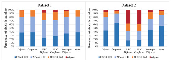
Figure 12.
Refinement comparison of the cost (color difference) intervals on both sides of the seamline for the six methods of Dataset 1 and Dataset 2. The bar chart shows the percentage of seamline pixels in each interval.
We can define as Dataset 3 and Dataset 4 very large remote sensing images because their number of image elements exceeds 100 million. In the face of such a large number of pixels, several algorithms “failed” in both dataset results. We take 3 h as the limit, and consider an algorithm that does not obtain a seamline after 3 h as “algorithm failure.” From the results, we can see that the graph cut algorithm and the two algorithms with SLIC super-pixel division both show “algorithm failure” for the two very large datasets. On the contrary, our algorithm can still compute the optimal seamline in the face of such a large amount of image elements. This benefits from the application of our proposed idea of down-sampling, where these images with very large data volumes can be simplified in our algorithm. Moreover, by comparing methods that are effective in the face of huge computational volume, our algorithm also presents better results in terms of computation time, color difference between the two sides of the mosaic line, and the number of features crossed.
By comparing the six different methods, we can analyze the advantages and disadvantages of our algorithm, as shown in Table 4. We can see that our method takes into account the three indicators of time consumption, color difference, and number of traversed features. In terms of time consumption, our method has a great advantage; in the case of color difference, our method is comparable to the optimal graph cut method; in the matter of number of traversed features, our method is inferior to the SLIC method in some experiments, but our method may have better results in some images. All of the above analyses are supported by the quantitative results shown in Table 3 and Figure 12.
Table 4.
Comparison of algorithm advantages and disadvantages.
5. Conclusions
In consideration of some existing satellite remote sensing images of huge data volume, it is challenging to mosaic these very large remote sensing images. In this paper, we propose a mosaic optimization method for oversized remote sensing images to synthesize seamless oversized remote sensing images. The whole workflow has the following three main steps: zoom in on the original image to obtain the first rough stitching line; generate band overlapping regions on the original image, and apply the graph cut algorithm for the second time to find the pixel-level optimal seamline; tessellation and mosaic along the seamline to obtain a seamless mosaic of oversized remote sensing images. The proposed method was tested using four different remote sensing images and six different methods for comparison and analysis. Based on the experimental results, we can draw the following conclusions:
- (1)
- Our method is generally applicable to a wide range of remote sensing images, and the optimal seamlines can be automatically generated for remote sensing images with different relative locations and different feature information.
- (2)
- The idea of using reduced images is useful for very large remote sensing images, which may determine the feasibility of the algorithm; for other remote sensing images, our method’s computational efficiency is more advantageous than the other algorithms.
- (3)
- The proposed algorithm produces excellent results for both computational efficiency and color difference between the two sides of the seamline. It is better than the original methods using only graph cut or Dijkstra and the inclusion of super-pixels.
Although our method can efficiently obtain the optimal seamlines from very large remote sensing images well, the method still needs some improvements. For example, our method can do the job of finding the relatively optimal seamline with minimal color difference between the two sides, but has a disadvantage in bypassing obvious features.
Author Contributions
Conceptualization, J.C. and X.C.; methodology, J.C. and X.C.; software, J.C. and X.C.; data analysis, J.C. and X.C.; investigation, J.C. and X.C.; resources, Z.M. and Q.Z.; writing X.C. and J.C.; supervision, J.C.; project administration, J.C.; funding acquisition, J.C. All authors have read and agreed to the published version of the manuscript.
Funding
This research was funded by NSFC-Zhejiang Joint Fund for the Integration of Industrialization and Informatization (Grant U1609202), the Project of State Key Laboratory of Satellite Ocean Environment Dynamics, Second Institute of Oceanography (No. SOEDZZ2203), the National Key Research and Development Program of China (Grant 2016YFC1400903), and National Natural Science Foundation of China (Grants 40606040, 41376184 and 40976109).
Data Availability Statement
Not applicable.
Conflicts of Interest
The authors declare no conflict of interest.
References
- Burt, P.J.; Adelson, E.H. A multiresolution spline with application to image mosaics. ACM Trans. Graph. 1983, 2, 217–236. [Google Scholar] [CrossRef]
- Kass, M.; Witkin, A.; Terzopoulos, D. Snakes: Active contour models. Int. J. Comput. Vis. 1988, 1, 321–331. [Google Scholar] [CrossRef]
- Williams, D.J.; Shah, M. A fast algorithm for active contours and curvature estimation. CVGIP Image Underst. 1992, 55, 14–26. [Google Scholar] [CrossRef]
- Li, X.; Hui, N.; Shen, H.; Fu, Y.; Zhang, L. A robust mosaicking procedure for high spatial resolution remote sensing images. ISPRS J. Photogramm. Remote Sens. 2015, 109, 108–125. [Google Scholar] [CrossRef]
- Pan, J.; Fang, Z.; Chen, S.; Ge, H.; Hu, F.; Wang, M. An improved seeded region growing-based seamline network generation method. Remote Sens. 2018, 10, 1065. [Google Scholar] [CrossRef]
- Yin, H.; Li, Y.; Shi, J.; Jiang, J.; Li, L.; Yao, J. Optimizing Local Alignment along the Seamline for Parallax-Tolerant Orthoimage Mosaicking. Remote Sens. 2022, 14, 3271. [Google Scholar] [CrossRef]
- Pan, J.; Wang, M.; Li, D.; Li, J. Automatic generation of seamline network using area Voronoi diagrams with overlap. IEEE Trans. Geosci. Remote Sens. 2009, 47, 1737–1744. [Google Scholar] [CrossRef]
- Pang, S.; Sun, M.; Hu, X.; Zhang, Z. SGM-based seamline determination for urban orthophoto mosaicking. ISPRS J. Photogramm. Remote Sens. 2016, 112, 1–12. [Google Scholar] [CrossRef]
- Pan, J.; Yuan, S.; Li, J.; Wu, B. Seamline optimization based on ground objects classes for orthoimage mosaicking. Remote Sens. Lett. 2017, 8, 280–289. [Google Scholar] [CrossRef]
- Zheng, M.; Xiong, X.; Zhu, J. A novel orthoimage mosaic method using a weighted A* algorithm–Implementation and evaluation. ISPRS J. Photogramm. Remote Sens. 2018, 138, 30–46. [Google Scholar] [CrossRef]
- Kerschner, M. Seamline detection in colour orthoimage mosaicking by use of twin snakes. ISPRS J. Photogramm. Remote Sens. 2001, 56, 53–64. [Google Scholar] [CrossRef]
- Dijkstra, E.W. A note on two problems in connexion with graphs. Numer. Math. 1959, 1.1, 269–271. [Google Scholar] [CrossRef]
- Chon, J.; Kim, H.; Lin, C.S. Seam-line determination for image mosaicking: A technique minimizing the maximum local mismatch and the global cost. ISPRS J. Photogramm. Remote Sens. 2010, 65, 86–92. [Google Scholar] [CrossRef]
- Ma, H.; Sun, J. Intelligent optimization of seam-line finding for orthophoto mosaicking with LiDAR point clouds. J. Zhejiang Univ. Sci. C 2011, 12, 417–429. [Google Scholar] [CrossRef]
- Hart, P.E.; Nilsson, N.J.; Raphael, B. A formal basis for the heuristic determination of minimum cost paths. IEEE Trans. Syst. Sci. Cybern. 1968, 4, 100–107. [Google Scholar] [CrossRef]
- Yu, L.; Holden, E.J.; Dentith, M.C.; Zhang, H. Towards the automatic selection of optimal seam line locations when merging optical remote-sensing images. Int. J. Remote Sens. 2012, 33, 1000–1014. [Google Scholar] [CrossRef]
- Zhang, J.; Sun, M.; Zhang, Z. Automated Seamline Detection for Orthophoto Mosaicking Based on Ant Colony Algorithm. Geomat. Inf. Sci. Wuhan Univ. 2009, 6, 675–678. (In Chinese) [Google Scholar]
- Ma, D.L.; Ding, N.; Cui, J. Optimizing ortho-image mosaic seamline based on Ant Colony algorithm. Sci. Surv. Mapp. 2013, 38. [Google Scholar]
- Wang, Q.; Zhou, G.; Song, R.; Xie, Y.; Luo, M.; Yue, T. Continuous space ant colony algorithm for automatic selection of orthophoto mosaic seamline network. ISPRS J. Photogramm. Remote Sens. 2022, 186, 201–217. [Google Scholar] [CrossRef]
- Soille, P. Morphological image compositing. IEEE Trans. Pattern Anal. Mach. Intell. 2006, 28, 673–683. [Google Scholar] [CrossRef]
- Pan, J.; Wang, M.; Li, J.; Yuan, S.; Hu, F. Region change rate-driven seamline determination method. ISPRS J. Photogramm. Remote Sens. 2015, 105, 141–154. [Google Scholar] [CrossRef]
- Li, L.; Yao, J.; Lu, X.; Tu, J.; Shan, J. Optimal seamline detection for multiple image mosaicking via graph cuts. ISPRS J. Photogramm. Remote Sens. 2016, 113, 1–16. [Google Scholar] [CrossRef]
- Li, L.; Tu, J.; Gong, Y.; Yao, J.; Li, J. Seamline network generation based on foreground segmentation for orthoimage mosaicking. ISPRS J. Photogramm. Remote Sens. 2019, 148, 41–53. [Google Scholar] [CrossRef]
- Yuan, Y.; Fang, F.; Zhang, G. Superpixel-based seamless image stitching for UAV images. IEEE Trans. Geosci. Remote Sens. 2020, 59, 1565–1576. [Google Scholar] [CrossRef]
- Yang, J.; Liu, L.; Yan, Q.; Deng, F. Efficient Seamline Network Generation for Large-Scale Orthoimage Mosaicking. IEEE Geosci. Remote Sens. Lett. 2022, 19, 1–5. [Google Scholar] [CrossRef]
- Chen, Q.; Sun, M.; Hu, X.; Zhang, Z. Automatic seamline network generation for urban orthophoto mosaicking with the use of a digital surface model. Remote Sens. 2014, 6, 12334–12359. [Google Scholar] [CrossRef]
- Zheng, M.; Xiong, X.; Zhu, J. Automatic seam-line determination for orthoimage mosaics using edge-tracking based on a DSM. Remote Sens. Lett. 2017, 8, 977–986. [Google Scholar] [CrossRef]
- Zhang, Y.; Zhang, M.; Du, S.; Zou, Z. Seamline optimisation for urban aerial ortho-image mosaicking using graph cuts. Photogramm. Rec. 2018, 33, 131–147. [Google Scholar] [CrossRef]
- Wan, Y.; Wang, D.; Xiao, J.; Lai, X.; Xu, J. Automatic determination of seamlines for aerial image mosaicking based on vector roads alone. ISPRS J. Photogramm. Remote Sens. 2013, 76, 1–10. [Google Scholar] [CrossRef]
- Wang, D.; Cao, W.; Xin, X.; Shao, Q.; Brolly, M.; Xiao, J.; Wan, Y.; Zhang, Y. Using vector building maps to aid in generating seams for low-attitude aerial orthoimage mosaicking: Advantages in avoiding the crossing of buildings. ISPRS J. Photogramm. Remote Sens. 2017, 125, 207–224. [Google Scholar] [CrossRef]
- Zheng, M.; Zhou, S.; Xiong, X.; Zhu, J. A novel orthoimage mosaic method using the weighted A* algorithm for UAV imagery. Comput. Geosci. 2017, 109, 238–246. [Google Scholar] [CrossRef]
- Boykov, Y.; Veksler, O.; Zabih, R. Fast approximate energy minimization via graph cuts. IEEE Trans. Pattern Anal. Mach. Intell. 2001, 23, 1222–1239. [Google Scholar] [CrossRef]
- Boykov, Y.; Kolmogorov, V. An experimental comparison of min-cut/max-flow algorithms for energy minimization in vision. IEEE Trans. Pattern Anal. Mach. Intell. 2004, 26, 1124–1137. [Google Scholar] [CrossRef] [PubMed]
- Adler-Golden, S.M.; Matthew, M.W.; Bernstein, L.S.; Levine, R.Y.; Berk, A.; Richtsmeier, S.C.; Acharya, P.K.; Anderson, G.P.; Felde, G.; Gardner, J.; et al. Atmospheric correction for shortwave spectral imagery based on MODTRAN4. Imaging Spectrom. V SPIE 1999, 3753, 61–69. [Google Scholar]
- Smith, P.R. Bilinear interpolation of digital images. Ultramicroscopy 1981, 6, 201–204. [Google Scholar] [CrossRef]


Disclaimer/Publisher’s Note: The statements, opinions and data contained in all publications are solely those of the individual author(s) and contributor(s) and not of MDPI and/or the editor(s). MDPI and/or the editor(s) disclaim responsibility for any injury to people or property resulting from any ideas, methods, instructions or products referred to in the content. |
© 2022 by the authors. Licensee MDPI, Basel, Switzerland. This article is an open access article distributed under the terms and conditions of the Creative Commons Attribution (CC BY) license (https://creativecommons.org/licenses/by/4.0/).