Toward a Real-Time Analysis of Column Height by Visible Cameras: An Example from Mt. Etna, in Italy

Alvaro Aravena; Giuseppe Carparelli; Raffaello Cioni; Michele Prestifilippo; Simona Scollo

doi:10.3390/rs15102595

Abstract

Volcanic plume height is one the most important features of explosive activity; thus, it is a parameter of interest for volcanic monitoring that can be retrieved using different remote sensing techniques. Among them, calibrated visible cameras have demonstrated to be a promising alternative during daylight hours, mainly due to their low cost and low uncertainty in the results. However, currently these measurements are generally not fully automatic. In this paper, we present a new, interactive, open-source MATLAB tool, named ‘Plume Height Analyzer’ (PHA), which is able to analyze images and videos of explosive eruptions derived from visible cameras, with the objective of automatically identifying the temporal evolution of eruption columns. PHA is a self-customizing tool, i.e., before operational use, the user must perform an iterative calibration procedure based on the analysis of images of previous eruptions of the volcanic system of interest, under different eruptive, atmospheric and illumination conditions. The images used for the calibration step allow the computation of ad hoc expressions to set the model parameters used to recognize the volcanic plume in new images, which are controlled by their individual characteristics. Thereby, the number of frames used in the calibration procedure will control the goodness of the model to analyze new videos/images and the range of eruption, atmospheric, and illumination conditions for which the program will return reliable results. This also allows improvement of the performance of the program as new data become available for the calibration, for which PHA includes ad hoc routines. PHA has been tested on a wide set of videos from recent explosive activity at Mt. Etna, in Italy, and may represent a first approximation toward a real-time analysis of column height using visible cameras on erupting volcanoes.

Keywords:

eruption column height; image analysis; Etna volcano; visible cameras; MATLAB

1. Introduction

Multiple volcanic hazards are associated with tephra dispersal [1,2,3], which encourages volcanological observatories to permanently improve their monitoring systems with the aim of tracking the main features of an explosive eruption [4,5,6,7]. Eruption column height is one of the most important source parameters for volcanic monitoring purposes [8,9]. In fact, this parameter is reported in the VONA (Volcano Observatory Notices for Aviation) messages issued in real-time by volcano observatories when an ash-producing event occurs and/or when there is a change in volcanic behavior [10]. The VONA messages are usually sent by fax or email by the observatory to the pertinent Area Control Centre, Meteorological Watch Office, and Volcanic Ash Advisory Centre [10]. Plume height estimation is also essential to evaluate the mass eruption rate of an explosive event [11,12,13,14], and represents a critical factor in forecasting volcanic ash dispersion [15,16,17] through numerical modeling [18,19,20,21,22]. Moreover, the level reached by the volcanic plume is essential in some gas plumes and aerosol retrievals by satellite [4]. Eruption column height can be obtained using different remote sensing techniques, including satellite [23,24,25], thermal or visible video cameras [4,26,27], radar [28,29,30,31], and Lidar [32,33,34]. However, in some circumstances, discrepancies among results from different instruments can occur [35,36]. Satellite systems, for example, may fail when the volcanic plume is not optically thick enough [4], whereas the quality of radar retrievals could depend on different factors such as the volcanic particle size [37].

Recent studies have demonstrated that the use of calibrated visible cameras seem promising and is becoming a useful tool from a volcano monitoring perspective [4]. Cameras in the visible band are able to detect volcanic plumes during daylight hours. It is a very low-cost system when compared to others and allows, in case of an eruption, measurement of the plume height directly from the images [4]. However, plume height estimation from visible cameras is often not automatic and needs an operator to manually sign the height variation with time. Although the error estimations may be less than 5% [4], automatic retrievals of volcanic plume from low-cost visible cameras could reduce the time analysis and lessen the hazard during explosive eruptions. In fact, if the plume height is retrieved automatically, its value could be used in data assimilation procedures needed for a reliable forecast of ash dispersal. Nowadays, while image-processing algorithms have been developed to detect, track, and extract the main parameters of convective plumes from thermal cameras [38,39], automatic procedures to analyze volcanic plume height from visible cameras are scarce [6] and they are not yet implemented for monitoring purposes. In this sense, it is worth noting that, currently, data assimilation techniques of volcanic plume dispersal are mainly based on satellite data [40,41] and we retain that the use of both satellite and ground-based data could really improve the results of volcanic ash dispersal forecasts [42].

Mount Etna (Sicily, Italy) is one of the most active volcanoes in the world, characterized by both effusive and explosive events that can be enclosed in a range that spans from long lasting, low intensity manifestations to paroxysmal phases with a short duration [43,44]. These eruptions may produce a high quantity of volcanic particles and, depending on the atmospheric conditions, fine ash can reach long distances from the summit craters [45]. Moreover, such particles represent a risk for the population and buildings of the neighboring areas, as well as for air traffic, airports, and other critical infrastructures [8,46]. For this reason, during the last ten years, many tools have been developed at the Istituto Nazionale di Geofisica e Vulcanologia, Osservatorio Etneo (INGV-OE) with the aim of detecting the main features of volcanic plumes and the prevention of hazard from tephra fallout [4,8,47]. In this sense, considering that column height estimates from calibrated visible cameras were added by the volcanologist on duty in the VONA messages during the recent Etna activity in 2021–2022, the automatic estimation of this value is a desirable task at INGV-OE, and results can be extended to other observatories around the world. In this paper, we present an interactive, open-source MATLAB tool designed to analyze images of volcanic eruptions derived from visible cameras, and to automatically recognize the temporal evolution of the volcanic plume height. Even though PHA is not an operative instrument for monitoring purposes yet, the code presented here may represent a first approximation toward a real-time analysis of column height using visible cameras on erupting volcanic systems.

This paper is organized as follows: in Section 2, we briefly describe the camera network of INGV-OE (Section 2.1) and the methodology used to detect the volcanic plume and automatically estimate the column height (Section 2.2). In Section 3, we show the main results focusing our attention on some test cases and on the construction of a code that is able to analyze images with different eruption, atmospheric, and illumination conditions. Finally, in Section 4 and Section 5, we discuss the main findings, limitations, and future advances associated with this program.

2. Materials and Methods

2.1. Camera Network of INGV-OE and Dataset

The surveillance network of Etna, whose data are managed by the INGV-OE, includes seismic and infrasonic stations, tiltmeters, GPS (global positioning systems), strainmeters, UV scanners, and thermal and visible cameras [48], among other instruments installed for monitoring purposes. In particular, the visible camera network of INGV-OE includes two low-cost visible cameras: EBVH (Etna Bronte Visible High-definition camera) and ECV (Etna Catania Visible camera), which sit in the west flank of Etna near the town of Bronte and in the southern flank of Etna in Catania, respectively. These cameras (model VIVOTEK IP8172P) present a maximum resolution of 2560 × 1920, with a field-of-view of 33°–93° (vertical), 24°–68° (horizontal), and 40°–119° (diagonal). The cameras are calibrated in terms of location and orientation [49]. With this information, assuming that the plume has a negligible depth and is confined to a vertical plane that rotates according to the wind direction, it is possible to manually estimate the height associated with each pixel of the images and thus calculate the plume height from the record of visible cameras [4], with uncertainties of the order of 0.5 km. Additional details can be found in Scollo et al. [4,49]. Specifically, the dataset considered in this work consists of videos recorded by the ECV static camera for different explosive eruptions (Table 1). This dataset includes both eruptions with optimal visibility conditions and eruptions where column height is not detectable, even manually (Table 1).

Table 1. Dataset of videos of camera ECV considered in this work. These events are sourced from the South East Crater (SEC).

2.2. Method for the Detection of Plume Height: The Program PHA

PHA (Plume Height Analyzer) is an open-source MATLAB tool that is able to analyze images and videos of volcanic eruptions (derived from visible cameras), with the objective of detecting the volcanic plume and calculation of the temporal evolution of plume height. The Image Processing Toolbox of MATLAB is required for launching the program PHA, whose graphical interface includes six sections (see Table 2). PHA is a self-customizing model, which means that the user must perform an iterative calibration procedure based on the analysis of images of previous eruptions before the model can be used to automatically detect plume height from new images. The underlying, final goal of this approach is to create a ‘universal’ functional algorithm that would automatically work for new eruptions (without further calibration), thus dealing with different eruption, atmospheric, and illumination conditions. Such a functionality would open the doors for us to implement real-time procedures to compute the column height of ongoing eruptions from the analysis of visible cameras.

Table 2. Summary of functions present in the PHA program.

For each frame analyzed (e.g., Figure 1a), the general procedure to compute the plume height consists of a series of successive steps (Figure 1):

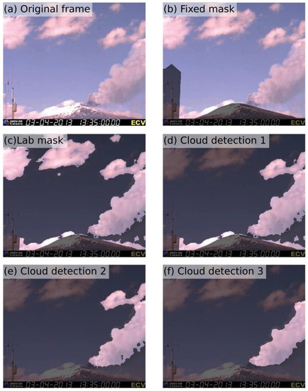
Figure 1. Illustrative example of the application of the procedures used to identify the plume in the program PHA. (a) Original image. (b) Application of the fixed mask. (c) Application of the Lab mask. (d–f) Application of the different algorithms aimed at discarding the clouds from the image.

(a): Application of a fixed mask to identify and discard the zones of the images associated with infrastructure (e.g., buildings, antennas, etc.) and volcano topography (Figure 1b, see Section 2.2.1).
(b): Subsequent use of a mask to identify and discard the zones of the images associated with the sky. This mask is mainly based on the analysis of the images in Lab scale (Figure 1c, see Section 2.2.2) and requires the development of the model calibration.
(c): The application of three successive procedures to identify and discard clouds, including those in contact with the plume (Figure 1d–f).
(d): A procedure to evaluate the internal variability of the non-masked zone of the images and eventually exclude the low-variability zones.
(e): Finally, considering a pixel-to-height conversion matrix (Figure 2), the highest pixel belonging to the plume is identified.

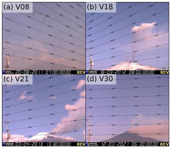Figure 2. Examples of the pixel-height conversion matrix used in this work. They are based on the dominant wind field observed during four events of Mount Etna (see titles and Table 1) [4]. Winds blowing to the E (to the right in the images) translate into height isocurves dipping to the W, while when winds blow to the W (to the left in the images), the resulting height isocurves dip to the E. Data are presented in m a.s.l.

In this section, we present in detail each one of the described steps, together with all the interactive functions that PHA includes for their development (see Table 2).

2.2.1. Fixed Mask

Given a static camera, a fixed mask is introduced (Figure 1b) in order to discard all the pixels of the images that are associated with infrastructure and volcano topography. This is important to avoid processing pixels whose properties are not associated with the eruption and/or atmospheric characteristics. Since this process must be performed only once for each static camera, the best way to define this mask is manually. For this, PHA includes ad hoc functions that allow creating interactively, saving, loading, and plotting the fixed mask (Table 2).

2.2.2. Lab Mask

We have observed that the third channel of an image in Lab scale (i.e., the color dimension b) generally discriminates well between clear sky pixels and other zones of the processed frames (e.g., volcanic plume and clouds; Figure 2c). The suitability of this channel to recognize sky pixels under optimal illumination conditions is similar to that observed by considering the subtraction of the red and the blue channels of the image in RGB scale, which is used in the software PlumeTraP [6], while it is slightly better during sunrise and sunset. For most frames of the studied videos, we have observed that a threshold value for the third channel of the image in Lab scale can be set in order to create a mask to split the image in two regions (hereafter, the Lab mask). However, it is not possible to set a single threshold value that works for a large set of images. Instead, it depends on specific image characteristics, which are in turn controlled by atmospheric factors as well as eruption and illumination conditions. Due to this, we developed an iterative procedure (hereafter, the Lab calibration) to calculate a function that, for each analyzed frame, provides the threshold (

T

) used to compute the Lab mask. This calibration can be performed using a reference video, a folder of videos, or a folder of images, and consists of an iterative procedure where different frames are sampled and analyzed, and the user is asked to indicate the best conservative mask (i.e., not masking the plume) from a choice of nine alternatives (Figure 3). Let us consider a calibration procedure based on

N

frames. For each frame (

i = 1, \dots, N

), and considering the portion of the images not masked by the fixed mask, the algorithm saves the following information:

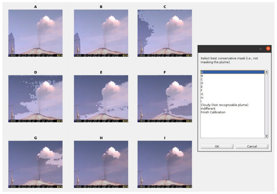
Figure 3. Illustrative example of the iterative procedure used to define the threshold value of the Lab mask, necessary to recognize the pixels belonging to the volcanic plume as a function of the image properties. In these images, the lightened areas correspond to pixels potentially considered as part of the ash plume. In this case, the recommended choice is E or F.

-: Mean value of L (Lab scale, $L_{i}$ ).
-: Mean value of a (Lab scale, $a_{i}$ ).
-: Mean value of b (Lab scale, $b_{i}$ ).
-: Mean value of R (RGB scale, $R_{i}$ ).
-: Mean value of G (RGB scale, $G_{i}$ ).
-: Mean value of B (RGB scale, $B_{i}$ ).
-: Threshold ( $T_{i}$ ).

The properties of the

i

-th calibration image are thus given by

X_{i} = {L_{i}, a_{i}, b_{i}, R_{i}, G_{i}, B_{i}}

and the information provided by the user, by selecting the best conservative mask, is given by

T_{i}

. Using

X_{i}

and distance-based criteria, calibration images are automatically clustered. The number of clusters (

M

) clearly depends on

N

: the larger the set of calibration images, the higher the number of clusters. The use of weighted, distance-based clustering techniques allows automatically generating classes of images characterized by common eruption, atmospheric, and illumination conditions. In this procedure, the distance between the different frames is computed by adopting the vector

X_{i}

associated with each of them to define their positions. For each cluster, a specific function is derived to calculate the threshold (

T

) used in the Lab mask:

T = F_{j} (X) = F_{j} ({R, G, B, L, a, b})

where

j

is a subscript referring to the cluster (i.e.,

j = 1, \dots, M

).

F_{j}

is defined using a polynomial fit computed by adopting the subset of calibration images that defines the

j

–th cluster. The order of this polynomial fit depends on the amount of data available in this cluster (first order regression for clusters with 20 data or less, and second order regression for clusters with more than 20 data). We also assume that

F_{j} (X)

is bounded by the minimum and maximum thresholds within the calibration images.

Thus, when a new image is analyzed, characterized by the vector

X_{n}

, the code finds its cluster by computing the minimum distance between

X_{n}

and

X_{i}

(

i = 1, \dots, N

), and then it adopts the function

F_{j}

associated with this specific cluster to calculate

F_{j} (X_{n})

. On the other hand, a calibration function defined by the nearest calibration frame (in terms of the image characteristics, that is, in terms of the vector

X_{i}

) is also present in PHA. To present conservative results, in this work we use the more conservative choice between both the alternatives for each frame analyzed.

The number of iterations determines the spectrum of images that the code will be able to analyze correctly. Since this is a critical factor in the effectiveness of the presented procedure, PHA includes a set of functions that allows creating and interactively improving the calibration data, as well as for loading, comparing, and testing them (Table 2). We remark that the only relevant correction needed by the Lab mask is associated with dark zones of the plume during sunrise and sunset, but this is automatically solved with no need of calibration. Additionally, note that this iterative procedure allows the user to indicate the images where the plume is not recognizable, which permits the code to automatically identify the images where the estimation of plume height is not possible using visible cameras (e.g., cloudy conditions, night images).

2.2.3. Cloud Identification

At this point, in general, the algorithm has masked all but the plume and clouds. Three successive procedures are then employed to discard the pixels associated with clouds:

(a): We trace a large number of segments between border points of the image (above the vent position) including both horizontal and inclined segments. When a line intersecting a completely masked zone is identified (i.e., with no plume or clouds), the entire region above this line is masked, reducing the computation time and discarding pixels associated with clouds (Figure 1d).
(b): Then, all the not masked pixels are clustered considering a distance-based criterion, and only the nearest cluster to the volcanic vent is conserved for the following steps (Figure 1e).
(c): Finally, the perimeter of the non-masked region is studied to identify lobe-like geometries. When the distance (calculated through a line) between two points in the non-masked region border is much lower than the distance calculated through the perimeter of this region, these points are assumed to define a lobe-like geometry, and this part of the non-masked zone is discarded. In this way, clouds superposed to the plume tend to be discarded (Figure 1f).

Since this procedure needs the volcanic vent position as an input parameter, PHA includes a set of functions that allow to interactively set the position of the vent (note that the definition of vent position must be performed only once for each static camera). The program allows plotting and loading this information as well (Table 2).

2.2.4. Internal Variability of Non-Masked Zone

At this point, the algorithm has identified a set of pixels that represent a good candidate for the volcanic plume. However, sometimes the limits of the plume are diffuse, and thus we need an additional criterion. Since color variability tends to be higher in the plume, we adopted a threshold to consider the portion of the mask characterized by a large color variability. A fixed threshold value has works for all the videos studied here, and thus calibration is not needed. In any case, PHA includes proper functions to set different values of threshold when it is required (e.g., for other volcanoes or other static cameras).

2.2.5. Pixel to Height Conversion

In order to calculate plume height, we need a procedure that is able to relate pixels to plume height. This is represented by a conversion matrix with the same dimensions of the images, indicating the height associated with each pixel of the image. In this way, the model is able to evaluate the height of all the pixels belonging to the plume and determine the plume height (i.e., the maximum height associated with a plume pixel). While PHA offers different alternatives to create a conversion matrix (see Table 2), in this work we use specific conversion matrixes associated with the wind fields observed during some of the eruptions described here (see Section 2.1 and Figure 2). The frames studied present a maximum measurement height of the order of 10 km a.s.l. due to limitations in the field view, which is influenced by wind direction and intensity as well. Whereas winds blowing to the E (to the right in the images) translate into height isocurves dipping to the W, when winds blow to the W (to the left in the images), the height isocurves dip to the E. On the other hand, winds blowing to the south (i.e., directly towards the ECV camera) produce more spaced height isocurves (i.e., reduction in the measurement limit) and winds blowing to the north translate into less spaced height isocurves (i.e., increment of the measurement limit). Specific details about the geometric considerations needed to define these pixel-to-height conversion matrixes can be found in Scollo et al. [4,49].

2.2.6. Results

Once the information of each frame is computed, PHA plots the temporal evolution of height plume, excluding results considered outliers within the temporal series. Results are also saved in MATLAB files that can be imported, plotted, and compared later using the program PHA.

3. Test Examples and Results

3.1. Internal Calibrations

As a first step, we show examples of internal calibrations, i.e., we use a few frames of single videos to create a calibration file and then we apply it to analyze the same videos. We focus on three short videos with different degrees of complexity (V18, V08 and V21; see Table 1) and a long-lasting video with significant changes in eruption and illumination conditions (V30; see Table 1). Note that all the calibration files and results described in this paper are included in the Git repository https://github.com/AlvaroAravena/PHA (accessed on 12 January 2023).

3.1.1. V18 (18 March 2012)

This eruption is part of the 25 low-explosivity events observed at Etna between January 2011 and April 2012 [50]. V18 is characterized by extremely favorable illumination and atmospheric conditions. We performed three independent calibrations using only 5 frames out of 450 recorded over a 15 min period (calibration files V18_a-c).

In Figure 4, we show the evolution of the Lab threshold estimated using these three calibrations on the 450 frames of V18. We can note that the application of the different calibration files produces reasonably similar decreasing trends for the Lab threshold. Then, we used the same set of calibration files to analyze V18 with the pixel-to-height conversion matrix presented in Figure 2b (see Section 2.2.5). We highlight that, due to the optimal illumination and atmospheric conditions of V18, an even smaller number of calibration frames seems enough to produce reproducible numerical results and similar to manual estimates, as observed in Figure S1a in the Supplementary Material.

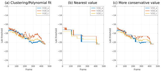
Figure 4. Threshold values for the Lab mask as a function of frame number of the video V18, computed using three different calibrations based on five frames extracted from V18 (see legends). In the different panels, we present the application of different fit strategies to define the threshold for the Lab mask. Results derived from the application of clustering and polynomial fit are presented in panel a, results in panel b are associated with a criterion of nearest value, and panel c presents, for each frame, the more conservative choice between panels a and b (i.e., the minimum value). Note that PHA (see Table 2) can generate this figure automatically.

The temporal evolutions of column height, calculated using the different calibration files, are strongly consistent between them (Figure 5a), showing percentage differences of the order of 0.2% during the video (maximum value of 1.0%). Note that similar average percentage differences are computed when numerical results are compared with manual estimates (Figure S1a). The results indicate a continuous increase in column height from ~6700 m up to ~8200 during these 15 min, with oscillations with a period of about 5 min (see Supplementary Videos S1–S3 in the Supplementary Material). The regularity in the evolution of plume height highlights the precision of this program under favorable atmospheric and illumination conditions.

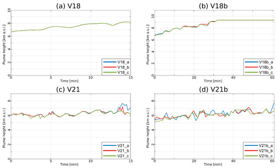
Figure 5. Plume height as a function of time for some reference videos (see titles) of Mt. Etna (see Table 1) using different files of internal calibration (see legends and Section 3.1). The measurement limit in panel b is 9326 m a.s.l.

We dispose of an additional set of 61 frames for a longer period (1 h) of the same eruption (V18b). Since a significant change in the eruption and illumination conditions occurs, the previous calibrations are not able to capture the characteristics of the complete video (note that it was recorded at 8 a.m.). In fact, these calibrations only work for the first ~35 frames of the video. Instead, we created three new, independent calibrations based on 5 frames out of 61 recorded over a period of 1 h (calibration files V18b_a–c). Results are consistent between them and show an increasing trend of plume height from ~6700 up to more than the measurement limit (Figure 5b and Supplementary Videos S4–S6). In this case, our calibrations produce average percentage differences of the order of 0.3% (0.5% before reaching the measurement limit), with a maximum value of 4.1%.

3.1.2. V21 (3 April 2013)

V21 is a video characterized by favorable illumination conditions and partially favorable atmospheric conditions due to the presence of several clouds that often cover part of the eruption plume. In this case as well, we performed three independent calibrations with only 5 frames out of 450 (calibration files V21_a–c), and then they were used to analyze the same video. The pixel-to-height conversion matrix is presented in Figure 2c (see Section 2.2.5). The evolution of plume height calculated using the different calibration files is similar (Figure 5c), showing oscillations between ~5800 and ~6800 m a.s.l. The only significant differences between numerical results are observed in a few, specific frames near the end of the video (differences of the order of 1000 m or less), when small clouds disturb the plume identification for two of the calibrations (see Supplementary Videos S7–S9). On average, the percentage differences of plume height associated with these calibrations are of the order of 1.3%. When compared with manual estimates, the average percentage differences of plume height are instead of the order of 3.0% (Figure S1b). Interestingly, Figure S1b shows a regular decrease in the average percentage difference with respect to manual estimates when the number of frames used for the Lab calibration increases, suggesting that a calibration based on >8 frames would produce a significantly better performance.

An additional video with 61 frames over a longer period of the same eruption was analyzed using three different calibrations based on only 5 frames (calibration files V21b_a–c). A general trend of plume height increase can be observed (from ~5300 to ~6900 m a.s.l.; Figure 5d). The main discrepancies between the curves are product of the interference of small clouds and the plume (instead, large clouds are typically recognized and discarded; see Supplementary Videos S10–S12). The percentage differences between the results obtained with these independent 5-frames-based calibrations are of the order of 2.8% (average value), with a maximum value of 11.5%. Interestingly, the calibrations constructed using a period of 15 min (i.e., calibration files V21_a–c) are able to capture well the characteristics of the complete video V21b (Supplementary Figure S2), reflecting that the illumination conditions are nearly constant during the 1 h video V21b (note that it was recorded at 1 p.m.).

3.1.3. V08 (20 August 2011)

V08 is also included in the sequence of 25 low-explosivity events observed at Etna between January 2011 and April 2012 [50]. This video presents partially unfavorable illumination and atmospheric conditions, with permanent presence of a strata of low-altitude clouds. We constructed three independent calibrations with 5 frames each (out of 900 frames), which were used to analyze the same video (calibration files V08_a-c). On the other hand, the matrix of pixel-to-height conversion of this video is presented in Figure 2a (see Section 2.2.5). The results produced by PHA, highly consistent between them, are characterized by a continuous increase in plume height up to reach the image top and thus exceed the measurement limit (Figure 6a). The increase in plume height occurs rapidly, at a rate of ~600 m/min, from ~4200 to ~9800 m a.s.l. Some of the calibrations differ in specific frames during the waxing phase due to the diffuse limits of the plume in this period (see Supplementary Videos S13–S15), while they capture well the general tendency of plume height. In this case, on average, the percentage differences of plume height are of the order of 0.3% (1.1% before reaching the measurement limit), with a maximum value of 11.5%. With respect to manual estimates, the average percentage differences are of the order of 3.0%, and we also observe a regular decrease in the average percentage difference with respect to manual estimates when the number of frames used for the Lab calibration increases (Figure S1c). Results suggest that, for this video, an internal calibration based on 5 frames is enough to produce reliable data of column height.

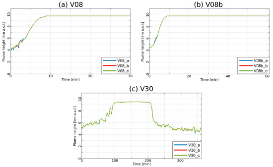
Figure 6. Plume height as a function of time for some reference videos (see titles) of Mt. Etna (see Table 1) using different files of internal calibration (see legends and Section 3.1). The measurement limit in panels a and b is 9774 m a.s.l. and that of panel c is 9517 m a.s.l.

The same set of calibrations was able to analyze the frames of the video V08b (Table 1), which comprises a longer period of the same eruption (Figure 6b). Results associated with the different calibration files (see Supplementary Videos S16–S18) are strongly consistent and capture well the characteristics of the waxing phase described in the previous paragraph.

3.1.4. V30 (12 March 2021)

V30 is a ~6-h-lasting video with strong changes in the illumination and eruption conditions, comprising well-defined waxing and waning phases. Consequently, a larger number of calibration frames must be considered in order to create a functional calibration file. We constructed three independent 10-frames-based calibrations (out of 361 frames), which were used to analyze the same video (Figure 6c and Supplementary Videos S19–S21). Our results, obtained by adopting the pixel-to-height conversion matrix presented in Figure 2d, show a waxing phase from a plume height of ~5200 m a.s.l. to a value beyond the measurement limit, with an average rate of plume height increase in the order of 40 m/min, much smaller than that observed in V08. Note, however, that the waxing phase can be divided in two steps with different variation rates of plume height (Figure 6c). The waning phase, from beyond the measurement limit up to a plume height of ~5500 m a.s.l., occurred at a rate of ~120 m/min and, after that, plume height decreases slowly up to ~4700 m a.s.l. The results obtained using the different calibrations are strongly similar, with average differences of the order of 2.0%, while average percentage differences of the order of 7.0% are obtained when numerical results are compared with manual estimates (Figure S1d). Note that at least 10 calibration frames are needed to obtain average percentage differences (with respect to manual measurements) below 10% (Figure S1d).

3.2. Operational Calibration

We have shown that PHA permits to analyze videos of volcanic eruptions by means of a fast calibration process. Although this may be useful for research and operative purposes by itself, an autonomous operative use of PHA requires that the program can recognize the characteristics of new images and estimate proper calibration parameters. In other words, in order to advance toward the implementation of a real-time column height estimation procedure using visible cameras on erupting volcanoes, we need a calibration file that considers a large set of eruption, illumination, and atmospheric conditions. To do this, PHA includes a set of functions that allows to create, merge, and improve calibrations by adding new data, permitting to refine the performance of the program as new data becomes available for the calibration as well (see Table 2).

To show the capability of the program to deal with a large calibration file and to recognize different conditions simultaneously, we merged a set of calibration files constructed using different videos (Table 1). Our dataset includes: (a) 5 frames for short-lasting videos with a capture period of 1 min (V08b, V18b, and V21b), (b) 10 frames for long-lasting videos with a capture period of 1 min (V30), (c) 40 frames for long-lasting videos with a capture period of 2 s (V26 and V29), and (d) 10 frames for short-lasting videos with a capture period of 2 s (all the other videos), totaling 375 frames. The application of a common calibration file for a large set of videos has shown that:

(a): For eruptions with favorable atmospheric conditions and when the outline of the plume is well defined (V02, V10, V12, V15, V18, V18b, V23, V28, V29, and V30), PHA is able to trace accurately plume height and in some cases small-scale oscillations of this parameter can be identified as well (Figure 7). Comparisons with manual estimates of plume height are presented in Figure 7, where we can observe remarkably consistent trends.

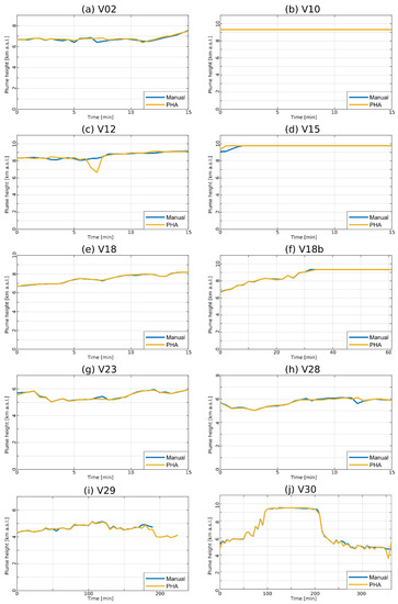Figure 7. Plume height as a function of time for some reference videos (see titles) of Mt. Etna (see Table 1), using a common calibration file (see Section 3.2). These videos are characterized by favorable atmospheric and illumination conditions, and the plumes present a well-defined outline.
(b): For eruptions with unfavorable atmospheric conditions (e.g., small clouds interfering the visual field; V06, V08, V08b, V14, V21, and V21b), the program is able to recognize well the range of values of plume height and general tendencies, but small-scale oscillations are not traced and occasional mistakes in punctual frames are observed. However, we stress that they are typically below the intrinsic uncertainty of plume height estimations based on visible cameras [4], as observed in Figure 8, where we present comparisons with manual estimates.

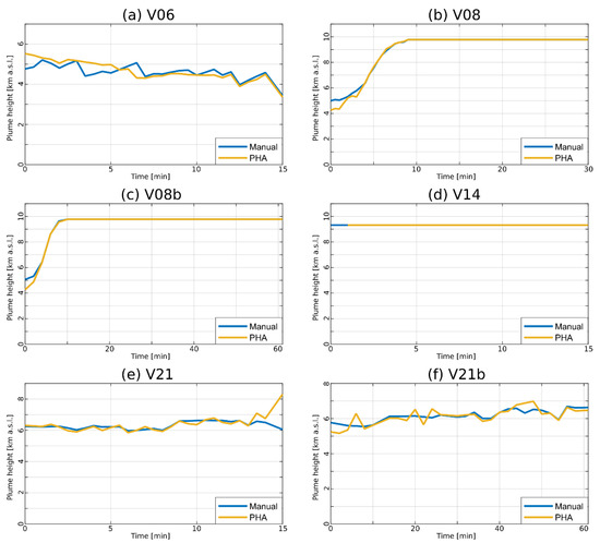Figure 8. Plume height as a function of time for some reference videos (see titles) of Mt. Etna (see Table 1), using a common calibration file (see Section 3.2). These videos are characterized by unfavorable atmospheric conditions (e.g., presence of clouds interfering with the visual field), and the plumes present a well-defined outline.
(c): Finally, for eruptions with plumes characterized by diffuse outlines (V01, V03, V04, V05, V09, V11 and V26), PHA is able to trace well the range of values of plume height and recognizes large-scale tendencies. However, the results present a typically oscillating behavior around the manual estimates (Figure 9) and occasional mistakes in specific frames are observed as well.

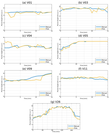Figure 9. Plume height as a function of time for some reference videos (see titles) of Mt. Etna (see Table 1), using a common calibration file (see Section 3.2). These videos are characterized by plumes with diffuse outlines.

In general terms, results are consistent with manual measurements, showing that PHA, when an enough large number of frames are present in the calibration file, is able to deal with different eruption, atmospheric, and illumination conditions. The average percentage difference between manual and automatic measurements of column height is 2.70%, with a median of 0.59% and 90th and 95th percentiles of 8.55% and 13.73%, respectively. Regarding the absolute difference between the two estimates of column height, the average value is 166.8 m, with a median of 34.5 m and with 90th and 95th percentiles of 548.0 m and 925.1 m, respectively.

4. Discussion

4.1. The Program PHA

In this paper, we have presented the program PHA, which is a novel, open-source MATLAB tool designed to analyze images from visible cameras of volcanic plumes, with the aim of automatically recognizing the plume and estimate its maximum height as a function of time. Due to the intrinsic variability of the images captured during volcanic eruptions, which is a consequence of changes in eruption, illumination, and atmospheric conditions, PHA was conceived as a self-customizing tool. This means that, before operational use, an iterative calibration procedure must be performed, based on the analysis of previous eruptions of the volcanic system of interest, possibly occurred under different environmental and volcanic conditions. The algorithm created to identify the volcanic plume largely relies on the analysis of the third channel of the images in Lab scale, which allows recognizing and discarding pixels associated with the sky, and the application of a series of procedures aimed at discarding clouds and determining high-color gradient zones in the plume.

By means of a series of illustrative applications of PHA on some events at Mt. Etna, Italy, we showed that a bounded number of frames can be used to calibrate the model and create a functional tool that is able to process data from past eruptions and trace the plume height automatically, with reproducible and accurate results when compared with manual measurements (see Section 3.1). However, to create a program that is able to recognize in real-time the characteristics of new images and estimate proper calibration parameters, a calibration with a large set of images with different characteristics in terms of illumination, atmospheric conditions, and eruption parameters, is needed. PHA includes a large set of interactive functionalities to facilitate the construction of a truly operative tool in the context of volcano monitoring, with functions to create, improve, and merge the data of different calibration files. In this paper, these functions were used to create a calibration file based on 375 images captured by the ECV visible camera of Etna. This calibration file has been shown to be useful to analyze videos of 23 events of Mt. Etna. Results are remarkably consistent with manual estimations when illumination and atmospheric conditions are favorable, while some occasional mistakes are still present when illumination and atmospheric conditions are not optimal. However, even in this case, the program permits to recognize large-scale, time-dependent tendencies of the eruptions, with differences between PHA and manual estimates typically below the intrinsic uncertainty of these measurements [4]. This first attempt shows that PHA is potentially useful to construct a tool that is able to analyze automatically visible camera images of Mt. Etna, with important applications for monitoring purposes, and may represent a significant approximation toward a real-time analysis of column height using visible cameras on erupting volcanoes.

4.2. Limitations, Strengths, and Future Advances of PHA

This tool presents the intrinsic limitations of images of visible cameras: reliable results can be obtained exclusively during daylight hours and with a small to moderate presence of clouds. They also present a bounded visual field, which translated into the presence of measurement limits as those observed in the ECV visible camera of Mt. Etna (see Figure 5, Figure 6, Figure 7, Figure 8 and Figure 9). On the other hand, due to the frequent presence of clouds in the summit of stratovolcanoes, this tool cannot be directly used to recognize the onset of an explosive eruption. In fact, the current version of the code does not include an automatic procedure to detect the absence of an ash plume and, in such a case, it will only indicate that the plume height, if present, is less than the minimum measurement limit.

Additionally, a calibration step is strictly needed before its use and, even if this tool can be set to analyze a posteriori the record of visible cameras from any explosive volcanic eruption, the availability of large datasets of past eruptions is necessary to construct an operative tool in real-time for monitoring purposes. Thus, this type of application is only feasible in volcanoes with frequent and well-monitored volcanic activity such as Etna, where the need of having a rapid, reliable tool to detect and measure volcanic plumes represents an impelling necessity.

Even though PHA is still not an operative instrument at INGV-OE, the results presented in this paper are encouraging in terms of the applicability of a customizable tool to estimate plume height as a function of time for monitoring purposes. To further improve the performance of PHA, the inclusion of additional videos of past eruptions is needed, as well as more code reliability testing and analysis of videos from other volcanoes with enough eruptions recorded. Additionally, the structure of the code allows for the refinement of the model by including new variables that are able to characterize the calibration frames (i.e., increasing the dimensions of the vector

X_{i}

; see Section 2.2.2); thus improving the characteristics of the fit used to calculate the calibration-derived inputs. We emphasize that this code can also be adapted to analyze images from thermal cameras, which uncovers additional development opportunities for this code in the future.

5. Conclusive Remarks

A new open-source MATLAB tool named Plume Height Analyzer’ (PHA) able to analyze images from visible cameras of volcanic plumes and automatically estimate its maximum height as a function of time is presented in this paper. Although the tool uses an iterative calibration procedure based on the analysis of previous eruptions of a given volcano and should be tested under different environmental and volcanic conditions, it may represent a first approximation toward a real-time analysis of column height using visible cameras on erupting volcanoes.

Supplementary Materials

The following supporting information can be downloaded at: https://www.mdpi.com/article/10.3390/rs15102595/s1. Figure S1: Average percentage difference with respect to manual measurements of column height for a set of results obtained with the program PHA, as a function of the number of frames used for the construction of the calibration files adopted (internal calibration). For each video (see titles), we created fifteen independent calibration files with different numbers of calibration frames (from 2 to 10 in panels a-c, from 4 to 20 in panel d). In each panel, we present the mean value (filled circles) and standard deviation (bars) associated with the application of three independent calibration files, created using different numbers of calibration frames (see x-axis). Figure S2: Plume height as a function of time for video V21b of Etna (see Table 1) using different files of internal calibration (see legends and Section 3.1). Video S1: Video V18 analyzed using the calibration file V18_a. Video S2: Video V18 analyzed using the calibration file V18_b. Video S3: Video V18 analyzed using the calibration file V18_c. Video S4: Video V18b analyzed using the calibration file V18b_a. Video S5: Video V18b analyzed using the calibration file V18b_b. Video S6: Video V18b analyzed using the calibration file V18b_c. Video S7: Video V21 analyzed using the calibration file V21_a. Video S8: Video V21 analyzed using the calibration file V21_b. Video S9: Video V21 analyzed using the calibration file V21_c. Video S10: Video V21b analyzed using the calibration file V21b_a. Video S11: Video V21b analyzed using the calibration file V21b_b. Video S12: Video V21b analyzed using the calibration file V21b_c. Video S13: Video V08 analyzed using the calibration file V08_a. Video S14: Video V08 analyzed using the calibration file V08_b. Video S15: Video V08 analyzed using the calibration file V08_c. Video S16: Video V08b analyzed using the calibration file V08_a. Video S17: Video V08b analyzed using the calibration file V08_b. Video S18: Video V08b analyzed using the calibration file V08_c. Video S19: Video V30 analyzed using the calibration file V30_a. Video S20: Video V30 analyzed using the calibration file V30_b. Video S21: Video V30 analyzed using the calibration file V30_c.

Author Contributions

Conceptualization, R.C. and S.S; methodology, A.A., G.C., R.C., M.P. and S.S; software, A.A. and G.C.; writing—original draft preparation, A.A. and G.C.; Writing—review and editing, A.A., G.C., R.C., M.P. and S.S. All authors have read and agreed to the published version of the manuscript.

Funding

This work was also in the framework of the INGV Project “Pianeta Dinamico” (D53J19000170001), funded by MUR ("Ministero dell'Università e della Ricerca, Fondo finalizzato al rilancio degli investimenti delle amministrazioni centrali dello Stato e allo sviluppo del Paese, legge 145/2018”).

Data Availability Statement

The data used in this paper belong to INGV and can be made available upon request to the authors.

Acknowledgments

The program PHA is available online via the webpage https://www.github.com/AlvaroAravena/PHA (accessed on 12 January 2023).

Conflicts of Interest

The authors declare no conflict of interest.

References

Bonadonna, C.; Connor, C.B.; Houghton, B.F.; Connor, L.; Byrne, M.; Laing, A.; Hincks, T.K. Probabilistic modeling of tephra dispersal: Hazard assessment of a multiphase rhyolitic eruption at Tarawera, New Zealand. J. Geophys. Res. Solid Earth 2005, 110, 2896. [Google Scholar] [CrossRef]
Wilson, T.M.; Stewart, C.; Sword-Daniels, V.; Leonard, G.S.; Johnston, D.M.; Cole, J.W.; Wardman, J.; Wilson, G.; Barnard, S.T. Volcanic ash impacts on critical infrastructure. Phys. Chem. Earth Parts A/B/C 2012, 45, 5–23. [Google Scholar] [CrossRef]
Craig, H.; Wilson, T.; Stewart, C.; Outes, V.; Villarosa, G.; Baxter, P. Impacts to agriculture and critical infrastructure in Argentina after ashfall from the 2011 eruption of the Cordón Caulle volcanic complex: An assessment of published damage and function thresholds. J. Appl. Volcanol. 2016, 5, 7. [Google Scholar] [CrossRef]
Scollo, S.; Prestifilippo, M.; Bonadonna, C.; Cioni, R.; Corradini, S.; Degruyter, W.; Rossi, E.; Silvestri, M.; Biale, E.; Carparelli, G.; et al. Near-Real-Time Tephra Fallout Assessment at Mt. Etna, Italy. Remote Sens. 2019, 11, 2987. [Google Scholar] [CrossRef]
Perttu, A.; Taisne, B.; De Angelis, S.; Assink, J.D.; Tailpied, D.; Williams, R.A. Estimates of plume height from infrasound for regional volcano monitoring. J. Volcanol. Geotherm. Res. 2020, 402, 106997. [Google Scholar] [CrossRef]
Simionato, R.; Jarvis, P.A.; Rossi, E.; Bonadonna, C. PlumeTraP: A New MATLAB-Based Algorithm to Detect and Parametrize Volcanic Plumes from Visible-Wavelength Images. Remote Sens. 2022, 14, 1766. [Google Scholar] [CrossRef]
Vásconez, F.; Moussallam, Y.; Harris, A.J.; Latchimy, T.; Kelfoun, K.; Bontemps, M.; Macías, C.; Hidalgo, S.; Córdova, J.; Battaglia, J.; et al. VIGIA: A thermal and visible imagery system to track volcanic explosions. Remote Sens. 2022, 14, 3355. [Google Scholar] [CrossRef]
Scollo, S.; Prestifilippo, M.; Spata, G.; D'Agostino, M.; Coltelli, M. Monitoring and forecasting Etna volcanic plumes. Nat. Hazards Earth Syst. Sci. 2009, 9, 1573–1585. [Google Scholar] [CrossRef]
White, J.T.; Connor, C.B.; Connor, L.; Hasenaka, T. Efficient inversion and uncertainty quantification of a tephra fallout model. J. Geophys. Res. Solid Earth 2017, 122, 281–294. [Google Scholar] [CrossRef]
Lechner, P.; Tupper, A.; Guffanti, M.; Loughlin, S.; Casadevall, T. Volcanic Ash and Aviation—The Challenges of Real-Time, Global Communication of a Natural Hazard; Advances in Volcanology Series; Springer: Cham, Switzerland, 2017; pp. 51–64. [Google Scholar] [CrossRef]
Sparks, R. The dimensions and dynamics of volcanic eruption columns. Bull. Volcanol. 1986, 48, 3–15. [Google Scholar] [CrossRef]
Mastin, L.G.; Guffanti, M.; Servranckx, R.; Webley, P.; Barsotti, S.; Dean, K.; Durant, A.; Ewert, J.W.; Neri, A.; Rose, W.I.; et al. A multidisciplinary effort to assign realistic source parameters to models of volcanic ash-cloud transport and dispersion during eruptions. J. Volcanol. Geotherm. Res. 2009, 186, 10–21. [Google Scholar] [CrossRef]
Degruyter, W.; Bonadonna, C. Improving on mass flow rate estimates of volcanic eruptions. Geophys. Res. Lett. 2012, 39, 2566. [Google Scholar] [CrossRef]
Mereu, L.; Scollo, S.; Garcia, A.; Sandri, L.; Bonadonna, C.; Marzano, F.S. A New Radar-Based Statistical Model to Quantify Mass Eruption Rate of Volcanic Plumes. Geophys. Res. Lett. 2023, 50, e2022GL100596. [Google Scholar] [CrossRef]
Tupper, A.; Textor, C.; Herzog, M.; Graf, H.; Richards, M. Tall clouds from small eruptions: The sensitivity of eruption height and fine ash content to tropospheric instability. Nat. Hazards 2009, 51, 375–401. [Google Scholar] [CrossRef]
Denlinger, R.P.; Pavolonis, M.; Sieglaff, J. A robust method to forecast volcanic ash clouds. J. Geophys. Res. Atmos. 2012, 117. [Google Scholar] [CrossRef]
Bonadonna, C.; Folch, A.; Loughlin, S.; Puempel, H. Future developments in modelling and monitoring of volcanic ash clouds: Outcomes from the first IAVCEI-WMO workshop on Ash Dispersal Forecast and Civil Aviation. Bull. Volcanol. 2012, 74, 1–10. [Google Scholar] [CrossRef]
Searcy, C.; Dean, K.; Stringer, W. PUFF: A high-resolution volcanic ash tracking model. J. Volcanol. Geotherm. Res. 1998, 80, 1–16. [Google Scholar] [CrossRef]
Stohl, A.; Forster, C.; Frank, A.; Seibert, P.; Wotawa, G. The Lagrangian particle dispersion model FLEXPART version 6.2. Atmos. Chem. Phys. 2005, 5, 2461–2474. [Google Scholar] [CrossRef]
Costa, A.; Macedonio, G.; Folch, A. A three-dimensional Eulerian model for transport and deposition of volcanic ashes. Earth Planet. Sci. Lett. 2006, 241, 634–647. [Google Scholar] [CrossRef]
Tadini, A.; Roche, O.; Samaniego, P.; Guillin, A.; Azzaoui, N.; Gouhier, M.; de' Michieli Vitturi, M.; Pardini, P.; Eychenne, J.; Bernard, B.; et al. Quantifying the uncertainty of a coupled plume and tephra dispersal model: PLUME-MOM/HYSPLIT simulations applied to Andean volcanoes. J. Geophys. Res. Solid Earth 2020, 125, e2019JB018390. [Google Scholar] [CrossRef]
Aravena, A.; Bevilacqua, A.; Neri, A.; Gabellini, P.; Ferrés, D.; Escobar, D.; Aiuppa, A.; Cioni, R. Scenario-based probabilistic hazard assessment for explosive events at the San Salvador Volcanic complex, El Salvador. J. Volcanol. Geotherm. Res. 2023, 438, 107809. [Google Scholar] [CrossRef]
Rose, W.I.; Bluth, G.J.S.; Ernst, G.G. Integrating retrievals of volcanic cloud characteristics from satellite remote sensors: A summary. Philos. Trans. R. Soc. Lond. Ser. A Math. Phys. Eng. Sci. 2000, 358, 1585–1606. [Google Scholar] [CrossRef]
Piscini, A.; Corradini, S.; Marchese, F.; Merucci, L.; Pergola, N.; Tramutoli, V. Volcanic ash cloud detection from space: A comparison between the RSTASH technique and the water vapour corrected BTD procedure. Geomat. Nat. Hazards Risk 2011, 2, 263–277. [Google Scholar] [CrossRef]
Prata, F.; Lynch, M. Passive Earth Observations of Volcanic Clouds in the Atmosphere. Atmosphere 2019, 10, 199. [Google Scholar] [CrossRef]
Andò, B.; Pecora, E. An advanced video-based system for monitoring active volcanoes. Comput. Geosci. 2006, 32, 85–91. [Google Scholar] [CrossRef]
Prata, A.J.; Bernardo, C. Retrieval of volcanic ash particle size, mass and optical depth from a ground-based thermal infrared camera. J. Volcanol. Geotherm. Res. 2009, 186, 91–107. [Google Scholar] [CrossRef]
Harris, D.M.; Rose, W.I.; Roe, R.; Thompson, M.R.; Lipman, P.; Mullineaux, D. Radar observations of ash eruptions. USA Geol. Surv. Prof. Pap. 1981, 1250, 323–333. [Google Scholar]
Vulpiani, G.; Ripepe, M.; Valade, S. Mass discharge rate retrieval combining weather radar and thermal camera observations. J. Geophys. Res. Solid Earth 2016, 121, 5679–5695. [Google Scholar] [CrossRef]
Marzano, F.S.; Picciotti, E.; Montopoli, M.; Vulpiani, G. Inside volcanic clouds: Remote sensing of ash plumes using microwave weather radars. Bull. Am. Meteorol. Soc. 2013, 94, 1567–1586. [Google Scholar] [CrossRef]
Montopoli, M. Velocity profiles inside volcanic clouds from three-dimensional scanning microwave dual-polarization Doppler radars. J. Geophys. Res. Atmos. 2016, 121, 7881–7900. [Google Scholar] [CrossRef]
Wiegner, M.; Gasteiger, J.; Groß, S.; Schnell, F.; Freudenthaler, V.; Forkel, R. Characterization of the Eyjafjallajökull ash-plume: Potential of lidar remote sensing. Phys. Chem. Earth Parts A/B/C 2012, 45, 79–86. [Google Scholar] [CrossRef]
Scollo, S.; Boselli, A.; Coltelli, M.; Leto, G.; Pisani, G.; Spinelli, N.; Wang, X. Monitoring Etna volcanic plumes using a scanning LiDAR. Bull. Volcanol. 2012, 74, 2383–2395. [Google Scholar] [CrossRef]
Sicard, M.; Córdoba-Jabonero, C.; Barreto, A.; Welton, E.J.; Gil-Díaz, C.; Carvajal-Pérez, C.V.; Torres, C. Volcanic eruption of Cumbre Vieja, La Palma, Spain: A first insight to the particulate matter injected in the troposphere. Remote Sens. 2022, 14, 2470. [Google Scholar] [CrossRef]
Tupper, A.; Wunderman, R. Reducing discrepancies in ground and satellite-observed eruption heights. J. Volcanol. Geotherm. Res. 2009, 186, 22–31. [Google Scholar] [CrossRef]
Corradini, S.; Montopoli, M.; Guerrieri, L.; Ricci, M.; Scollo, S.; Merucci, L.; Marzano, F.S.; Pugnaghi, S.; Prestifilippo, M.; Ventress, L.J.; et al. A multi-sensor approach for volcanic ash cloud retrieval and eruption characterization: The 23 November 2013 Etna lava fountain. Remote Sens. 2016, 8, 58. [Google Scholar] [CrossRef]
Marzano, F.S.; Vulpiani, G.; Rose, W.I. Microphysical characterization of microwave radar reflectivity due to volcanic ash clouds. IEEE Trans. Geosci. Remote Sens. 2006, 44, 313–327. [Google Scholar] [CrossRef]
Bombrun, M.; Jessop, D.; Harris, A.; Barra, V. An algorithm for the detection and characterisation of volcanic plumes using thermal camera imagery. J. Volcanol. Geotherm. Res. 2018, 352, 26–37. [Google Scholar] [CrossRef]
Wood, K.; Thomas, H.; Watson, M.; Calway, A.; Richardson, T.; Stebel, K.; Naismith, A.; Berthoud, L.; Lucas, J. Measurement of three dimensional volcanic plume properties using multiple ground based infrared cameras. ISPRS J. Photogramm. Remote Sens. 2019, 154, 163–175. [Google Scholar] [CrossRef]
Osores, S.; Ruiz, J.; Folch, A.; Collini, E. Volcanic ash forecast using ensemble-based data assimilation: An ensemble transform Kalman filter coupled with the FALL3D-7.2 model (ETKF-FALL3D version 1.0). Geosci. Model Dev. 2020, 13, 1–22. [Google Scholar] [CrossRef]
Pardini, F.; Corradini, S.; Costa, A.; Ongaro, T.E.; Merucci, L.; Neri, A.; Stelitano, D.; de’Michieli Vitturi, M. Ensemble-Based Data Assimilation of Volcanic Ash Clouds from Satellite Observations: Application to the 24 December 2018 Mt. Etna Explosive Eruption. Atmosphere 2020, 11, 359. [Google Scholar] [CrossRef]
Lu, S.; Lin, H.X.; Heemink, A.; Segers, A.; Fu, G. Estimation of volcanic ash emissions through assimilating satellite data and ground-based observations. J. Geophys. Res. Atmos. 2016, 121, 10971–10994. [Google Scholar] [CrossRef]
Branca, S.; del Carlo, P. Types of eruptions of Etna volcano AD 1670–2003: Implications for short-term eruptive behaviour. Bull. Volcanol. 2005, 67, 732–742. [Google Scholar] [CrossRef]
De Beni, E.; Behncke, B.; Branca, S.; Nicolosi, I.; Carluccio, R.; D’Ajello Caracciolo, F.; Chiappini, M. The continuing story of Etna’s New Southeast Crater (2012–2014): Evolution and volume calculations based on field surveys and aerophotogrammetry. J. Volcanol. Geotherm. Res. 2015, 303, 175–186. [Google Scholar] [CrossRef]
Kampouri, A.; Amiridis, V.; Solomos, S.; Gialitaki, A.; Marinou, E.; Spyrou, C.; Georgoulias, A.K.; Akritidis, D.; Papagiannopoulos, N.; Mona, L.; et al. Investigation of Volcanic Emissions in the Mediterranean: “The Etna–Antikythera Connection”. Atmosphere 2021, 12, 40. [Google Scholar] [CrossRef]
Scollo, S.; Coltelli, M.; Bonadonna, C.; Del Carlo, P. Tephra hazard assessment at Mt. Etna (Italy). Nat. Hazards Earth Syst. Sci. 2013, 13, 3221–3233. [Google Scholar] [CrossRef]
Alparone, S.; Andronico, D.; Lodato, L.; Sgroi, T. Relationship between tremor and volcanic activity during the Southeast Crater eruption on Mount Etna in early 2000. J. Geophys. Res. Solid Earth 2003, 108, 2241. [Google Scholar] [CrossRef]
Calvari, S.; Biale, E.; Bonaccorso, A.; Cannata, A.; Carleo, L.; Currenti, G.; Di Grazia, G.; Ganci, G.; Iozzia, A.; Pecora, E.; et al. Explosive paroxysmal events at Etna volcano of different magnitude and intensity explored through a multidisciplinary monitoring system. Remote Sens. 2022, 14, 4006. [Google Scholar] [CrossRef]
Scollo, S.; Prestifilippo, M.; Pecora, E.; Corradini, S.; Merucci, L.; Spata, G.; Coltelli, M. Eruption column height estimation of the 2011-2013 Etna lava fountains. Ann. Geophys. 2014, 57, 2. [Google Scholar] [CrossRef]
Behncke, B.; Branca, S.; Corsaro, R.A.; De Beni, E.; Miraglia, L.; Proietti, C. The 2011–2012 summit activity of Mount Etna: Birth, growth and products of the new SE crater. J. Volcanol. Geotherm. Res. 2014, 270, 10–21. [Google Scholar] [CrossRef]

Figure 1. Illustrative example of the application of the procedures used to identify the plume in the program PHA. (a) Original image. (b) Application of the fixed mask. (c) Application of the Lab mask. (d–f) Application of the different algorithms aimed at discarding the clouds from the image.

Figure 2. Examples of the pixel-height conversion matrix used in this work. They are based on the dominant wind field observed during four events of Mount Etna (see titles and Table 1) [4]. Winds blowing to the E (to the right in the images) translate into height isocurves dipping to the W, while when winds blow to the W (to the left in the images), the resulting height isocurves dip to the E. Data are presented in m a.s.l.

Figure 3. Illustrative example of the iterative procedure used to define the threshold value of the Lab mask, necessary to recognize the pixels belonging to the volcanic plume as a function of the image properties. In these images, the lightened areas correspond to pixels potentially considered as part of the ash plume. In this case, the recommended choice is E or F.

Figure 4. Threshold values for the Lab mask as a function of frame number of the video V18, computed using three different calibrations based on five frames extracted from V18 (see legends). In the different panels, we present the application of different fit strategies to define the threshold for the Lab mask. Results derived from the application of clustering and polynomial fit are presented in panel a, results in panel b are associated with a criterion of nearest value, and panel c presents, for each frame, the more conservative choice between panels a and b (i.e., the minimum value). Note that PHA (see Table 2) can generate this figure automatically.

Figure 5. Plume height as a function of time for some reference videos (see titles) of Mt. Etna (see Table 1) using different files of internal calibration (see legends and Section 3.1). The measurement limit in panel b is 9326 m a.s.l.

Figure 6. Plume height as a function of time for some reference videos (see titles) of Mt. Etna (see Table 1) using different files of internal calibration (see legends and Section 3.1). The measurement limit in panels a and b is 9774 m a.s.l. and that of panel c is 9517 m a.s.l.

Figure 7. Plume height as a function of time for some reference videos (see titles) of Mt. Etna (see Table 1), using a common calibration file (see Section 3.2). These videos are characterized by favorable atmospheric and illumination conditions, and the plumes present a well-defined outline.

Figure 8. Plume height as a function of time for some reference videos (see titles) of Mt. Etna (see Table 1), using a common calibration file (see Section 3.2). These videos are characterized by unfavorable atmospheric conditions (e.g., presence of clouds interfering with the visual field), and the plumes present a well-defined outline.

Figure 9. Plume height as a function of time for some reference videos (see titles) of Mt. Etna (see Table 1), using a common calibration file (see Section 3.2). These videos are characterized by plumes with diffuse outlines.

Table 1. Dataset of videos of camera ECV considered in this work. These events are sourced from the South East Crater (SEC).

ID	Date	Time (UTC)	Frames	Observations
V01	10 April 2011	08:00–08:15	450	Optimal atmospheric conditions. The outline of the plume is diffuse.
V02	10 April 2011	10:30–10:45	450	Favorable atmospheric conditions.
V03	12 May 2011	03:30–03:45	450	Favorable atmospheric conditions. The outline of the plume is diffuse. The images are particularly dark.
V04	12 May 2011	05:00–05:15	450	Favorable atmospheric conditions. The outline of the plume is diffuse during a portion of the video.
V05	9 July 2011	14:00–14:30	900	Unfavorable atmospheric conditions. The outline of the plume is diffuse during a portion of the video.
V06	25 July 2011	05:00–05:15	450	Partially favorable atmospheric conditions (presence of small clouds near the plume).
V07	25 July 2011	06:45–07:00	450	Weak plume with most of the ash spreading laterally ¹. Optimal atmospheric conditions.
V08	20 August 2011	07:00–07:30	900	Partially unfavorable atmospheric conditions.
V08b	20 August 2011	07:00–08:00	61	Partially unfavorable atmospheric conditions.
V09	29 August 2011	04:00–04:15	450	Poor visibility. The outline of the plume is diffuse.
V10	29 August 2011	04:30–04:45	450	Plume height is beyond the measurement limit during the whole video. The images are particularly reddish.
V11	8 September 2011	06:00–06:15	450	The outline of the plume is diffuse. Favorable atmospheric conditions.
V12	8 September 2011	07:30–07:45	450	Favorable atmospheric conditions.
V13	15 November 2011	10:00–10:15	450	No visibility ².
V14	15 November 2011	12:15–12:30	450	Unfavorable atmospheric conditions. Plume height is beyond the measurement limit during the whole video.
V15	5 January 2012	05:45–06:00	450	The images are particularly dark. Plume height is beyond the measurement limit during the whole video
V16	5 January 2012	13:00–13:15	450	Weak plume with most of the ash spreading laterally ¹.
V17	18 March 2012	05:00–05:15	450	Weak plume with most of the ash spreading laterally ¹.
V18	18 March 2012	08:00–08:15	450	Optimal atmospheric conditions.
V18b	18 March 2012	08:00–09:00	61	Optimal atmospheric conditions.
V19	28 February 2013	10:00–10:15	450	Poor visibility. A small portion of the plume is recognizable ².
V20	28 February 2013	10:30–10:45	450	Poor visibility. A small portion of the plume is recognizable ².
V21	3 April 2013	13:30–13:45	450	Partially favorable atmospheric conditions (presence of small clouds near the plume).
V21b	3 April 2013	13:00–14:00	61	Partially favorable atmospheric conditions (presence of small clouds near the plume).
V22	3 April 2013	16:00–16:15	450	Weak plume with most of the ash spreading laterally ¹. The outline of the plume is diffuse.
V23	12 April 2013	10:45–11:00	450	Favorable atmospheric conditions.
V24	12 April 2013	16:00–16:15	450	Weak plume with most of the ash spreading laterally ¹. The outline of the plume is diffuse.
V25	18 April 2013	08:00–08:15	450	Weak plume with most of the ash spreading laterally ¹. The outline of the plume is diffuse.
V26	18 April 2013	10:30–13:45	5850	The video includes a period with plume height beyond the measurement limit, while the outline of the plume is diffuse in the final part.
V27	27 April 2013	14:30–14:45	450	Weak plume with most of the ash spreading laterally ¹.
V28	27 April 2013	17:45–18:00	450	The images are particularly dark.
V29	19 April 2020	06:00–10:00	7200	Favorable atmospheric conditions.
V30	12 March 2021	06:35–12:10	361	The video includes a period with plume height beyond the measurement limit.

¹ Video employed to complement the set of calibration images used for the construction of an operative calibration file, but it was discarded for the analysis of plume height versus time because this parameter is not considered informative in this case. ² Video employed to complement the set of calibration images used for the construction of an operative calibration file, but it was discarded for the analysis of plume height versus time due to visibility limitations.

Table 2. Summary of functions present in the PHA program.

Section	Function	Description
Fixed mask	Load	Load a previously created fixed mask.
Fixed mask	Create	The program displays a graphical interface, where the user can draw a fixed mask on a reference image (selected by the user). This information is then saved in the folder MaskFiles.
Fixed mask	Plot	Plot the reference image and fixed mask.
Vent position	Load	Load a previously created vent position.
Vent position	Create	The program displays a graphical interface, where the user can select the vent position on a reference image (selected by the user). This information is then saved in the folder VentFiles.
Vent position	Plot	Plot the reference image, vent position and fixed mask.
Pixel to height	Load	Load a previously created pixel-height conversion matrix.
Pixel to height	Create	Three modalities to create a pixel-height conversion matrix are available: -Constant, vertical gradient: the user is asked to indicate the height associated with the vent and with the top of the reference image. -Bilinear interpolation: a graphical interface is displayed, and the user is asked to select a set of pixels of the image and indicate their heights. The resulting conversion matrix is computed by fitting this information as a function of pixel position, using a bilinear interpolation. -Second-order interpolation: a graphical interface is displayed, and the user is asked to select a set of pixels of the image and indicate their heights. The resulting conversion matrix is computed by fitting this information as a function of pixel position, using a second-order interpolation. The resulting pixel-height conversion matrix is saved in the folder PixelHeightFiles.
Pixel to height	Plot	Plot the reference image and the isolines of height, derived from the pixel-height conversion matrix.
Calibration: Lab mask	Load	Load a previously created calibration function.
Calibration: Lab mask	Create	An interactive, iterative procedure is launched, which samples frames from a calibration dataset provided by the user (a single video, a folder containing videos, or a folder containing images) and shows the application of different threshold values in the Lab mask (see Section 2.2.2). The user is asked to indicate the best conservative threshold value. Once the iteration is finished by the user, the program computes the functions used to calculate the Lab mask threshold as a function of the image properties (see Section 2.2.2). The resulting function is saved in the folder CalibrationFiles/LabMask.
Calibration: Lab mask	Improve	This routine reproduces the same process associated with the creation of a Lab mask calibration, but the information is added to an existent Lab mask calibration. Since the performance of this mask is strongly controlled by the amount of data that the calibration includes, this function allows to improve the program performance for a given static camera.
Calibration: Lab mask	Merge	This routine allows to merge the data contained in two or more existent Lab mask calibrations and creates a new, likely better calibration function.
Calibration: Lab mask	Test	An iterative procedure is launched that shows the application of the Lab mask, whose threshold is computed with the loaded calibration function, on a set of frames selected by the user (a single video, a folder containing videos, or a folder containing images).
Calibration: Lab mask	Compare	The user is asked to select two or more calibration functions (in order to compare them) and a set of frames (a single video or a folder of images). Two modalities are available: -Plot Threshold: the program calculates the Lab mask thresholds of the selected frames considering the different calibration functions. Then, this information is plotted. -Show images: an iterative procedure is launched that shows the application of different Lab masks, whose thresholds are computed using the selected calibration functions, on the set of frames indicated by the user.
Calibration: Default Parameters	Load	Load a previously created set of default parameters. Even though the results presented in this paper consider the same set of default parameters, this section allows to increase the applicability field of this code.
Calibration: Default Parameters	Create	A window is displayed, where the user can change some of the constant parameters used in the code (e.g., maximum number of clusters in Lab mask function). Even though the results presented in this paper consider the same set of default parameters, this section allows to increase the applicability field of this code.
Analysis	Single video	This function allows analyzing a single video. The user is asked to provide the frame step adopted to analyze the video and the time interval between two consecutives frames in the video. The output is a plot of the temporal evolution of plume height, and this information can be saved in the folder Results.
Analysis	Folder with images	This function allows analyzing a folder containing images. The user is asked to provide the time interval between two consecutives images. The output is a plot of the temporal evolution of plume height, and this information can be saved in the folder Results.
Analysis	Analyze manually	This function allows to select manually the pixel associated with the maximum height on a set of frames (a single video or a folder of images). The output is a plot of the temporal evolution of plume height, and this information can be saved in the folder Results.
Results	Single plot	This function allows plotting the results of previously analyzed videos/folders with images. The input of this function is the output file saved by any of the three functions of the section Analysis.
Results	Compare plots	This function allows comparing the results of previously analyzed videos/folders with images. The inputs of this function are the output files saved by any of the three functions of the section Analysis.

Disclaimer/Publisher’s Note: The statements, opinions and data contained in all publications are solely those of the individual author(s) and contributor(s) and not of MDPI and/or the editor(s). MDPI and/or the editor(s) disclaim responsibility for any injury to people or property resulting from any ideas, methods, instructions or products referred to in the content.

© 2023 by the authors. Licensee MDPI, Basel, Switzerland. This article is an open access article distributed under the terms and conditions of the Creative Commons Attribution (CC BY) license (https://creativecommons.org/licenses/by/4.0/).

Article Metrics

Citations

Article Access Statistics

Journal Statistics

Multiple requests from the same IP address are counted as one view.