Detection of Smoke from Straw Burning Using Sentinel-2 Satellite Data and an Improved YOLOv5s Algorithm

Abstract

The burning of straw is a very destructive process that threatens people’s livelihoods and property and causes irreparable environmental damage. It is therefore essential to detect and control the burning of straw. In this study, we analyzed Sentinel-2 data to select the best separation bands based on the response characteristics of clouds, smoke, water bodies, and background (vegetation and bare soil) to the different bands. The selected bands were added to the red, green, and blue bands (RGB) as training sample data. The band that featured the highest detection accuracy, RGB_Band6, was finally selected, having an accuracy of 82.90%. The existing object detection model cannot directly handle multi-band images. This study modified the input layer structure based on the YOLOv5s model to build an object detection network suitable for multi-band remote sensing images. The Squeeze-and-Excitation (SE) network attention mechanism was introduced based on the YOLOv5s model so that the delicate features of smoke were enhanced, and the Convolution + Batch normalization + Leaky ReLU (CBL) module was replaced with the Convolution + Batch normalization + Mish (CBM) module. The accuracy of the model was improved to 75.63%, which was 1.81% better than before. We also discussed the effect of spatial resolution on model detection and where accuracies of 84.18%, 73.13%, and 45.05% for images of 60-, 20-, and 10-m resolution, respectively, were realized. The experimental results demonstrated that the accuracy of the model only sometimes improved with increasing spatial resolution. This study provides a technical reference for the monitoring of straw burning, which is vital for both the control of straw burning and ways to improve ambient air quality.

1. Introduction

Biomass burning (BB) is defined as the open or quasi-open combustion of all non-fossil plant or organic fuels, including forest fires, crop residue burning, cooking fires, dung burning, etc. [1]. Open-air biomass burning (OBB) is a significant source of emissions of trace gaseous pollutants and carbonaceous particulate matter (PM) [2]. Open-crop straw burning is considered one of the main OBB types [3]. Shi et al. [4] conducted a systematic analysis of the state of straw handling and its utilization difficulties. They concluded that the reasons why straw burning is so widespread include: (1) low resource awareness among agricultural practitioners; (2) time-consuming and labor-intensive, insufficient efficiency drive, etc. The annual contribution of OBB to PM2.5 emissions is estimated to have increased significantly (191%) over the period 2002–2016 [5] and has a significant impact on global climate change [6]. Extensive, high-intensity open burning of straw can be detrimental to regional air quality as well as local public health and safety due to the large amounts of suspended particulate matter produced by straw burning [7], such as respirable particulate matter (PM10; aerodynamic diameter between 2.5 and 10 microns) and fine particulate matter (PM2.5; aerodynamic diameter less than 2.5 microns) [8]. These suspended particles affect tropospheric chemical processes and can cause chronic obstructive pulmonary diseases such as bronchitis and asthma [9]. Straw burning also causes the ground temperature to rise sharply, which not only destroys the living environment of beneficial microorganisms in the soil but also affects the absorption of soil nutrients by crops, reducing the yield and quality of crops on farmland.

At present, the monitoring of straw burning is based mainly on the detection of flames and smoke. The characteristics of the flame are prominent, and the detection of the flame is easier to realize than that of smoke detection. However, the flame is usually produced in the middle of the burning straw patch, so when the flame is detected, the fire is already extensive, and hence detection cannot play an effective role with respect to early warning [10]. As one of the most significant features of straw burning [11], smoke is used to detect the occurrence of straw burning [12]. Therefore, smoke is of great significance for controlling straw burning and improving ambient air quality.

There are currently three main methods used for smoke detection. One is to use various types of sensors; the second is to use a manual selection of smoke features first and then use image processing techniques for detection; and the third is to set up video acquisition equipment [13]. The first method is relatively straightforward, low-cost, and widespread in use. However, the sensor device eventually deteriorates or is damaged by the influence of the environment, so there are many missed and false cases of smoke detection [14]. The second method requires feature selection before detection. Manual feature selection relies primarily on experience and prior knowledge, which tend to trap the model in local optima and thus affect the accuracy of the smoke model [15]. The third method can provide relatively rapid positioning information and early warning when straw burning occurs. The video equipment must rely on the availability of long-term and stable power and network support; however, the lifetime of the electronic equipment is limited and it must be constantly updated and maintained [16], and the monitoring range of this equipment is minimal. By contrast, the technology associated with satellite remote sensing covers a large area, and the monitoring capability is simultaneous and economic, so observation of the Earth’s surface can be achieved. Thus, valuable data for detecting smoke from straw burning by remote sensing becomes possible [17]. To this end, there is an urgent need to develop robust algorithms for the detection of smoke associated with straw burning that are suitable for use with satellite remote sensing images.

Traditional smoke detection algorithms use features such as the color of the smoke and wavelet coefficients for extraction. Gubbi et al. [18] proposed a method that first decomposes the features of an image using wavelet variations, then the decomposed features are fused to describe the smoke, and finally a support vector machine (SVM) is used for classification. Chen et al. [19] analyzed the distribution of the color intensity of the smoke in the RGB and HIS spaces. They established a color model of the static characteristics of the smoke according to the distribution law. Li and Yuan [20] first extracted the local binary patterns (LBP) and the histogram of edge direction (EOH) features of the smoke, fused the two features, and then input them into the SVM for classification; the method achieved an accuracy of 86.5%. Xie et al. [21] constructed a multi-channel threshold method for smoke detection in forest fires using eight MODIS spectral channels based on the spectral analysis of different feature types. Zhao et al. [22] used MODIS data for smoke detection of forest fires based on spectral and spatial thresholding as well as uniform texture analysis. However, the above methods are not sufficiently adaptable for widespread use due to the computational complexity of feature selection, the uncertainty, and the difficulty in determining suitable thresholds [23].

With the development and advances in deep learning (DL), the detection algorithms can reduce hardware costs compared to traditional algorithms and eliminate the need for manual extraction of features [24]. Deep learning-based object detection algorithms can detect targets quickly, and YOLOv5s has been preferred due to its high detection speed [25]. However, although the YOLOv5s model is superior in detection speed, it has poorer detection accuracy. This study seeks to improve the YOLOv5s model to develop a high-accuracy detection model for smoke detection in straw burning that is applicable to Sentinel-2 remote sensing imagery.

Many current detection strategies for smoke based on satellite remote sensing imagery use MODIS data. However, Sentinel-2 can provide Earth observation data with superior spatial (10 m, 20 m, and 60 m) and temporal (5-day) resolution and richer surface information with broad application prospects [26]. In the present study, by analyzing the Sentinel-2 data, the combination of bands with the best separation was selected based on the response characteristics of clouds, smoke, water bodies, and background (vegetation and bare soil) for the different bands. Then the selected bands were added to the red, green, and blue bands as training sample data. However, existing object detection models cannot directly handle multi-band images. This study modifies the input layer structure based on the YOLOv5s model to address the current problem of building an object detection network applicable to multi-band remote sensing images. In this work, the Squeeze-and-Excitation (SE) network attention mechanism [27] was introduced to the original YOLOv5s model to improve the sensitivity of the model to smoke. In addition, the Convolution + Batch normalization + Leaky ReLU (CBL) module was replaced with the Convolution + Batch normalization + Mish (CBM) module [28] to speed up the convergence of the model and improve the accuracy of the network and the generalization ability.

The study explores the potential of Sentinel-2 remote sensing images in smoke detection, and we have sought to improve the accuracy of the YOLOv5s model for Sentinel-2 image smoke detection. The training of images with 10 m, 20 m, and 60 m spatial resolution, respectively, to analyze the influence of spatial resolution on model detection is discussed. This study not only provides a scientific basis for controlling the burning of straw but also for carrying out environmental monitoring and emergency management. Additionally, the work contributes to the study of the impact of human activities on the atmospheric environment, which is of great importance for combating climate change.

2. Materials and Methods

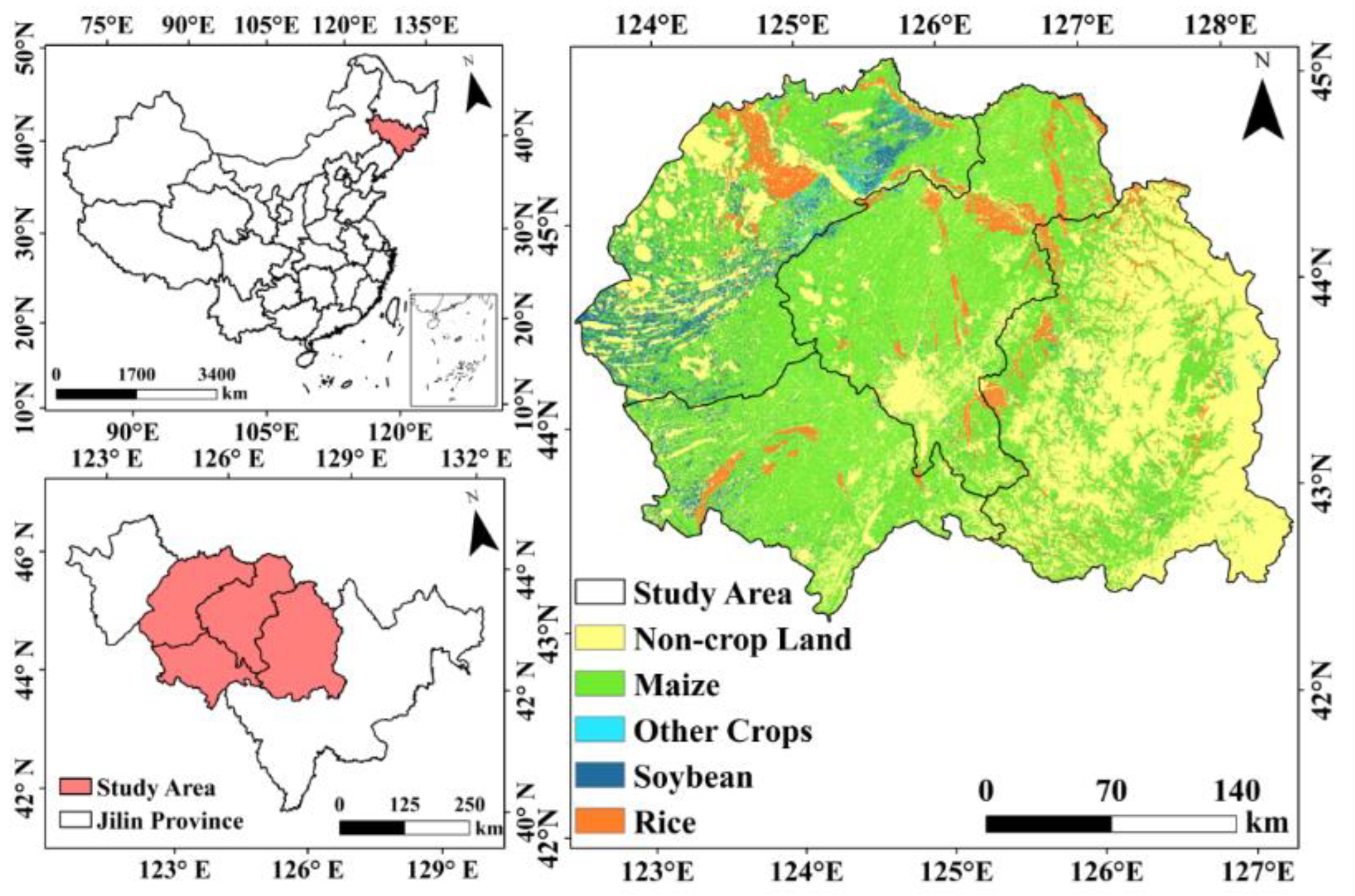
2.1. Overview of the Study Area

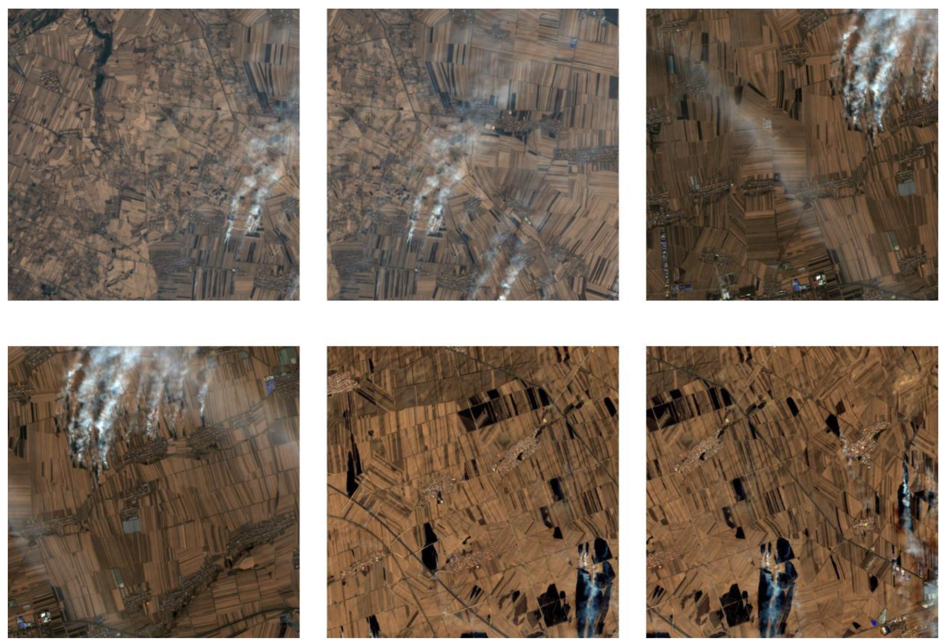
The study area was located in central Jilin Province, with geographical coordinates from 121°38′ to 131°19′E longitude and 40°50′ to 46°19′N latitude. The study area included the cities of Changchun, Jilin, Siping, and Songyuan, as shown in Figure 1.

The study area has a temperate continental monsoon climate with a distinct change of seasons, with short, warm, and rainy summers with average temperatures above 23 °C. Precipitation is abundant in the summer, with an annual average of 600 mm accounting for more than 60% of the annual precipitation. The study area is located in the northeastern plain, one of the three significant black soil plains; the soil type is dominated by black soil and black calcareous soil. The soils in the study area are neutral, with an average pH of 6.5 and an average organic matter content of 26.1 g∙kg⁻¹, which is favorable for crop growth due to their good soil properties and high fertility. Therefore, this area is a prominent grain-producing region in Jilin Province with a substantial commercial grain base [29] and makes an outstanding contribution to ensuring food security and stable social development in China. According to the Yearbook of Jilin Province in 2020 [30], the main crop types producing straw in the study area include maize, rice, and soybeans, with a total sown area of 3.12 million hectares, 0.49 million hectares, and 0.12 million hectares for these three crops, respectively. The annual production of straw in Jilin Province exceeds 40 million tons [31], and the straw resource output in the study area reached 10.87 t/hm², which clearly is a large amount of straw. However, the comprehensive utilization rate of straw is low [32].

The study area has severe winters with average temperatures below −11 °C, and there is a short time window for the straw to be returned to the field; thus, straw being discarded and burned at will is a very serious matter [33]. Due to the large-scale burning of straw in spring and autumn, acceptable PM2.5 levels increase by 0.5–4 times compared to other times of the year [34], seriously affecting the ambient air quality. In Changchun City in October 2017, the primary pollutant in the air, fine particulate matter PM2.5, was 68 micrograms per m³, a 33.3% increase over the same period in the previous year; also, the number of heavily polluted days increased by 3 days over the same period of the previous year. According to the analysis of Wang et al. [35], straw burning is an essential cause of the decline in ambient air quality in Changchun.

2.2. Data Sources

Sentinel-2 is a high-resolution multi-spectral imaging satellite carrying a multi-spectral imager (MSI) for terrestrial monitoring, providing images of vegetation, soil, water cover, inland waterways, and coastal areas, as well as for emergency services [26]. Sentinel-2 is divided into two satellites, 2A and 2B. Sentinel-2A was launched in June 2015, and Sentinel-2B in March 2017. With both satellites operating simultaneously, complete imaging of the Earth’s equatorial regions can be completed every five days. At the same time, for the higher latitudes of Europe, this cycle takes only three days [36]. The satellite covers 13 visible, near-infrared, and short-wave infrared spectral regions with spatial resolutions of 10, 20, and 60 m, respectively. It is a multi-spectral imaging satellite with high temporal and spatial resolution that can provide valuable data for smoke detection from straw burning. The band information for Sentinel-2 images is shown in Table S1 (Supplementary Material).

The Sentinel-2 data used in this study were downloaded from the European Space Agency (ESA) website (https://scihub.copernicus.eu/dhus/#/home, accessed on 15 October 2022). To create a dataset, four images containing smoke, clouds, vegetation, water bodies, and bare soil were selected. Given that straw burning occurs mainly in the months of April-May and October-November, the imaging period selected for this study was April-May and October-November from 2019 to 2021, and the data level is Level-2A. Level-1C is the radiometrically calibrated and geometrically corrected data. Moreover, Level-2A is the product of atmospheric corrections based on Level-1C [37]. The image information is shown in Figure 2.

2.3. Data Preprocessing

This study uses Sentinel-2 L2A level data and does not require radiometric calibration, geometric correction, or atmospheric correction operations [37]. The 13 bands of the Sentinel-2 image provide three spatial resolutions of 10 m, 20 m, and 60 m. To ensure consistent spatial resolution across the bands, all bands were resampled to the exact spatial resolution and output to ENVI (The Environment for Visualizing Images)-supported storage formats using the nearest-neighbor assignment method under the Sentinel Application Platform (SNAP) [38]. The band was then band-synthesized in ENVI. The input size supported by the YOLOv5s model is 640 × 640 pixels. Taking into account factors such as the experimental training time and the image size supported by the network structure, all four images were cropped to 640 × 640 pixels, and some examples are shown in Figure 3.

2.4. Dataset Construction

To better train the model, we annotated all smoke samples in the images after the cropping of the remote sensing data was undertaken. Samples were usually selected using visual interpretation methods, and the samples were labeled manually. We used the Labellmg annotation tool to label the smoke samples. Each line in the label file represents a markup box and has five values indicating the category of the markup content, the normalized center horizontal coordinate x, the normalized center vertical coordinate y, the normalized target box width w, and the normalized target box height h. The normalization of x and w refers to the center point horizontal coordinate and the width of the target box divided by the width of the image, respectively. The normalization of y and h refers to the center point vertical coordinate and the height of the target box divided by the height of the image, respectively.

Data enhancement operations were performed on the labeled images to increase the diversity within samples and avoid overfitting problems with the model. In this study, data enhancement of the cropped images containing a smoke plume was performed using a random combination of six enhancement methods: pan, rotate, mirror, add noise, cutout, and change brightness [39]. An original image was enhanced by five images, while a program was written to transform the corresponding annotation file for each image simultaneously, as shown in Figure 4.

After data enhancement was completed, the dataset was divided into the training set, the validation set, and the test set according to the ratio of 6:2:2. The final information is shown in

Table 1. Datasets for comparison experiments with different channel combinations as model inputs.

Channel Combination	Training Set	Test Set	Validation Set	Total Number
RGB (Red-Green–Blue, 10 m)	2431	810	819	4060
RGB_Band5 (10 m)	2431	810	819	4060
RGB_Band5_Band6 (10 m)	2431	810	819	4060
RGB_Band5_Band6_Band7 (10 m)	2431	810	819	4060
RGB_Band5_Band6_Band7_Band8 (10 m)	2431	810	819	4060
RGB_Band6 (10 m)	2431	810	819	4060
RGB_Band6_Band7 (10 m)	2431	810	819	4060
RGB_Band6_Band7_Band8 (10 m)	2431	810	819	4060
RGB_Band7 (10 m)	2431	810	819	4060
RGB_Band7_Band8 (10 m)	2431	810	819	4060
RGB_Band8 (10 m)	2431	810	819	4060

and

Table 2. Datasets with images of different spatial resolutions as model inputs.

Spatial Resolution	Training Set	Test Set	Validation Set	Total Number
60 m	2001	667	653	3321
20 m	2015	663	661	3339
10 m	2431	810	819	4060

.

To analyze the effect of different spatial resolutions on the detection results, we preprocessed the data with input band combinations of red-green-blue and spatial resolutions of 60 m, 20 m, and 10 m to produce the dataset in Table 2.

2.5. Improved YOLOv5s Model

YOLOv5s contains four sections: input, backbone, neck, and prediction. Backbone is primarily distinguished by its utilization of the focus slicing operation, which transforms information in the width-height plane into the channel dimension [40]. Then, convolution is utilized to extract characteristics and mitigate information loss caused by downsampling. The neck network is composed of the Feature Pyramid Network (FPN) [41] and Path Aggregation Network (PAN) [42] architectures. The FPN architecture passes high-level feature information through upsampling to convey robust semantic features. Meanwhile, the PAN is a feature pyramid that conveys robust positioning characteristics. The simultaneous employment of both architectures boosts the feature fusion capability of different layers and enhances the network’s capacity for multi-scale predictions.

Given that complex backgrounds characterize satellite-acquired remote sensing images, there is a slight contrast between the target and the background [43]. Some smoke samples occupy only a tiny area in the image, and problems such as missed or false detection can readily occur. To address these issues, we introduced the SE network attention mechanism in the Spatial Pyramid Pooling (SPP) module behind the backbone network [27]. This optimizes the activation function in the CBL structure by replacing the Leaky ReLU with the Mish [28] activation function. The Mish activation function is a non-linear activation function that is an extension of the ReLU activation function. It has a higher non-linear capability and can fit the data better. The existing object detection model cannot directly handle multi-band images. In this work, based on the YOLOv5s model, a program was written to modify the data acquisition part of the input [44] to build an object detection network applicable to multi-band remote sensing images. The structure of the improved YOLOv5s algorithm is shown in Figure 5.

The main improvements to the model include: (1) Previous research using YOLOv5s was mainly focused on the RGB optical images. This study increases the number of input channels according to the number of input bands to make the model applicable to input multispectral remote sensing images. (2) To address the problems of missed and false detection of small targets, this study introduces the SE attention mechanism, a classical attention mechanism widely used in industry. SE networks can use several small-scale sub-networks that automatically learn to derive a particular weight value to weigh all paths of the feature graph [27]. In DL neural networks, not all of the extracted features are essential. Using a recalibration method, the SE explicitly modeled the relationship between the feature channels to learn the weights of each channel. The SE promotes features with more useful weights and suppresses features with low weights. The SE model can improve the sensitivity of the model to the target [45] and reduce the negative impact of the complex background on the detection accuracy in smoke detection tasks, as shown in Figure S3 (Supplementary Material). (3) The Convolution + Batch normalization + Leaky ReLU (CBL) module of YOLOv5s uses the Leaky ReLU activation function [46], which is a segmented function with different interval functions and cannot provide consistent relational predictions for positive and negative input values. The present study is optimized by replacing the original activation function with the Mish activation function. The functional expression of the Mish activation function is given by Equation (S1) (Supplementary Material), and the derivative expression is given by Equation (S2) (Supplementary Material). The Mish function and its derivatives are continuous and smooth, so the Mish function is easier to gradient optimize and converges faster in backpropagation (BP) (see Figure S4 in the Supplementary Material).

2.6. Test Environment and Parameter Settings

Training and testing experiments were conducted on the same server with an AMD Ryzen 7 5800X3D 8-Core Processor manufactured by American semiconductor company, Advanced Micro Devices (AMD), headquartered in Santa Clara, CA, USA, an NVIDIA GeForce RTX 3080 Ti graphics card manufactured by American company NVIDIA, headquartered in Santa Clara, California, USA, and 32 GB of running memory. Using Pytorch 1.8 as the DL framework, all programs were written in Python, and the CUDA and OpenCV libraries were used to run under Windows.

During training, the learning rate was set to 0.01, the batch size was 4, the learning rate momentum was 0.937, SGD was used as the optimizer, the weight decay was set to 0.0005, and the number of iterations was 300.

2.7. Evaluation Indicators

The Intersect Over Union (IOU) threshold is directly related to the output prediction frame; generally, the larger the threshold, the higher the prediction accuracy [47]. The evaluation indicators used in this study included precision (P), recall (R), mean average precision at an IOU threshold of 0.5 (mAP50), frames per second (FPS), and FPS as the detection rate. The mAP is an essential measure of the accuracy of detection in an object detection model. P, R, and mAP were calculated using Equations (1)–(3), respectively.

$$\mathrm{P}=\frac{\mathrm{TP}}{\mathrm{TP}+\mathrm{FP}}$$

(1)

$$\mathrm{R}=\frac{\mathrm{TP}}{\mathrm{TP}+\mathrm{FN}}$$

(2)

$$\mathrm{mAP}=\frac{1}{\mathrm{K}}{{\displaystyle \sum }}_{\mathrm{K}=1}^{\mathrm{K}}\mathrm{AP}\left(\mathrm{P},\mathrm{R},\mathrm{K}\right)$$

(3)

where TP is a true positive, i.e., the number of positive samples detected as positive; FP is a false positive, i.e., the number of negative samples detected as positive; FN is a false negative, i.e., the number of positive samples detected as unfavorable; K is the number of target categories detected; and AP is the average precision, i.e., the area enclosed by the PR curve and the coordinate axis.

3. Results

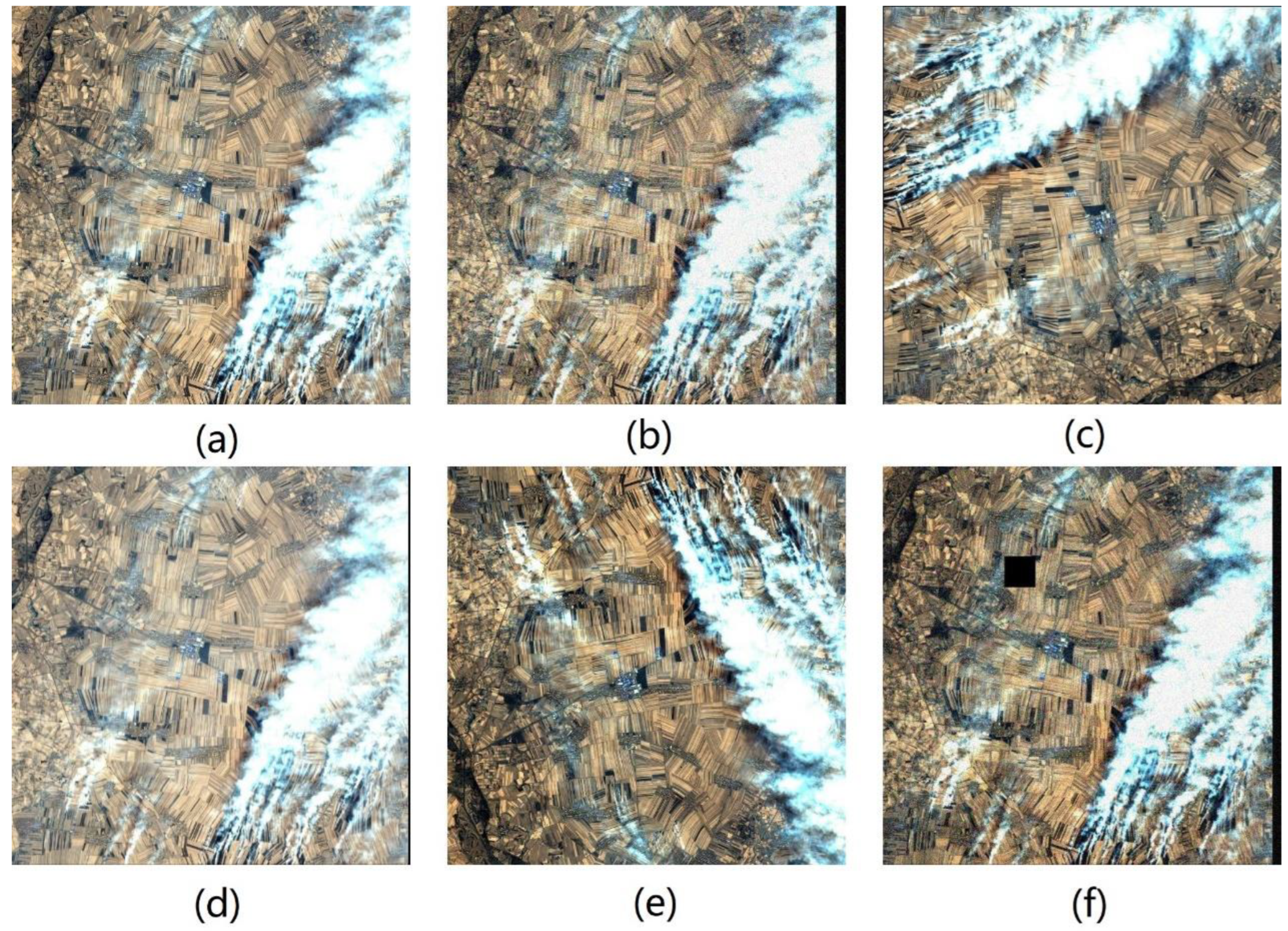
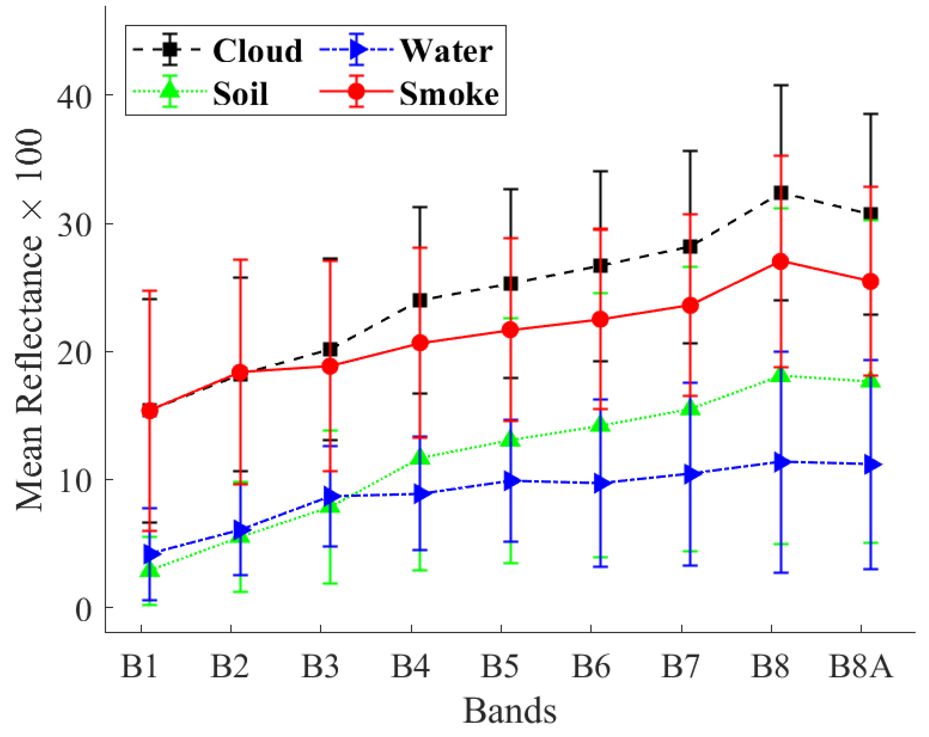
3.1. Separation Methods

The background of the smoke data is complex, and interference from clouds and backgrounds can cause the model to produce false alarms [48]. In this study, the other bands of Sentinel-2 will be added to the red, green, and blue bands as training sample data. The model’s ability to detect smoke is enhanced by adding input information to enrich the smoke features and reduce the interference of other feature types in smoke detection.

Sentinel-2 remote sensing imagery provides 13 spectral bands, all of which can be used to build models, resulting in significant data redundancy and also a significant increase in the computational cost of the model [49]. To select the feature vectors for the construction of the algorithm for the detection of smoke, spectral characterization of the different bands of Sentinel-2 was carried out. Li et al. [50] used a BP (backpropagation) neural network to identify smoke from forest fires. First, eight bands in the visible to near-infrared spectral regions of MODIS were analyzed, and bands 3, 7, and 8 were selected as feature vectors for the input layer of the BP neural network. After training, the Kappa coefficient for smoke detection using this algorithm was approximately 96.29%, so good detection results were realized. In the present study, nine bands (bands 1–8A) in the visible to near-infrared spectral regions of Sentinel-2 were selected for analysis, i.e., bands 1–8A were analyzed to assess the response characteristics of the ground objects, and the better bands were selected as the input for training the model.

Within the study area, four typical surface cover types were analyzed: smoke, clouds, water, and background, where background refers to the features of the underlying surface other than water. First, the cell points for the smoke, cloud, water, and background were extracted, and then the response of each spectral band was analyzed to obtain the sensitive channels for the smoke. The smoke detection model was henceforth constructed on this basis. Altogether, 300 sample cell points for each feature type (smoke, clouds, water, and background) were extracted from the images, with smoke based on the 4, 3, and 2-band composites of the Sentinel-2 images being used to classify the images. The classified sample cell elements for each feature type are presented in Figure 6.

The spectral response curves for the four ground object types in bands 1–8A are shown in Figure 7. As can be seen from the graph: (1) The reflectance of the potential smoke cells (real smoke and cloud cells) is higher than the reflectance of other features. (2) It is feasible to distinguish potential smoke pixels from other feature types based on the reflectance of channel 8 of Sentinel-2 because the smoke pixels have the highest reflectance in this channel, and the difference in reflectance is most significant amongst the other features. (3) The reflectivity values for the smoke and cloud elements almost overlap in bands 1 and 2, and those of the background and water elements almost overlap in band 3, so bands 1, 2, and 3 do not confer a good distinguishing capability between these four features.

The mean and standard deviation for each category were calculated from the reflectance of smoke and non-smoke sample pixels in bands 1–8A, and the values are listed in

Table 3. The mean values (reflectance × 100) and standard deviations for the four cover types.

Band	Variable	Smoke	Cloud	Background	Water
B1	Mean	15.37	15.38	2.86	4.17
	Std	9.39	8.75	2.63	3.63
B2	Mean	18.36	18.22	5.53	6.06
	Std	8.77	7.59	4.32	3.55
B3	Mean	18.85	20.13	7.88	8.69
	Std	8.23	7.09	5.98	3.90
B4	Mean	20.68	23.98	11.65	8.89
	Std	7.38	7.30	8.78	4.42
B5	Mean	21.70	25.43	13.05	9.90
	Std	7.17	7.38	9.58	4.77
B6	Mean	22.52	26.66	14.21	9.71
	Std	7.06	7.40	10.30	6.56
B7	Mean	23.60	28.17	15.49	10.42
	Std	7.07	7.52	11.14	7.15
B8	Mean	27.03	32.39	18.09	11.36
	Std	8.23	8.38	13.13	8.61
B8A	Mean	25.47	30.70	17.66	11.18
	Std	7.37	7.86	12.61	8.19

.

Usually, the normalized distance (H) [51] is used as an indicator for the selection of the waveband. The normalized distance (H) is given by Equation (4):

$$\mathrm{H}=\frac{\left|{\mathsf{\mu }}_1-{\mathsf{\mu }}_2\right|}{\left({\mathsf{\sigma }}_1+{\mathsf{\sigma }}_2\right)}$$

(4)

where ${\mathsf{\mu }}_i$ and ${\mathsf{\sigma }}_i$ are the mean and standard deviation of category i, respectively. A higher H value indicates a higher degree of separability and a more significant difference between the two categories; this indicator has been widely recognized and utilized [50]. The calculated H values between the three pairs of different features (smoke to cloud, smoke to background, and smoke to water) are shown in Figure 8. As can be seen from the graph, while the separation of smoke from the background and smoke from water is good in bands 1, 2, and 3, the separation of smoke from clouds is too low, with all values below 0.1. While band 8A has the highest separation of clouds from smoke, the separation of smoke from the background and smoke from water is 0.390 and 0.918, respectively, lower than the other bands. Therefore, in this study, bands 4–8, which afforded the best separation, were selected to distinguish between smoke and other feature types based on the separability of each band. Bands 4–8 were used as input to the YOLOv5s model in order to analyze the effect of the spectrum on the detection performance and to select the combination of bands with the best detection performance.

3.2. Comparison of Attention Models

To verify the effectiveness of the SE attention mechanism, the algorithm incorporating it [27] was compared with the algorithm without the attention mechanism and the algorithm incorporating the convolutional block attention module (CBAM) [52]. The experimental data for these groups used 20-m spatial resolution data, and the experimental results are shown in

Table 4. Comparison of detection capabilities with different attention mechanisms.

Attention Mechanism	Contraction Ratio	mAP50/%
None		77.27
SE	8	80.71
	16	76.66
	32	78.55
CBAM	8	69.36
	16	68.63
	32	65.72

.

As can be seen from Table 4, the addition of the SE attention mechanism resulted in the highest mAP50 of 80.71% for the model when the contraction ratio was 8. The addition of CBAM gave the highest mAP50 of 69.36% for the model at a contraction ratio of 8. Compared to the model without the addition of the attention mechanism, the addition of SE increased the mAP50 of the model by 3.44 percentage points, while the addition of CBAM decreased the mAP50 of the model by 7.91%. The findings show that the application of attention mechanisms in the model does not necessarily lead to improved detection accuracy; hence, the attention mechanism needs to be chosen according to the specific task.

3.3. Ablation Experiments

A comparison of the experimental results of the different versions of YOLOv5s is presented in

Table 5. Comparison of the performance of different versions of YOLOv5s in detecting smoke.

Model Used for Object Detection	P/%	R/%	mAP50/%
YOLOv5s	73.82	81.58	78.44
YOLOv5s − Mish	78.15	77.67	78.76
YOLOv5s + SE8	75.05	79.33	79.31
Improved YOLOv5s	75.63	81.00	82.49

. The experimental data for these groups used 20-m spatial resolution data. In YOLOv5s-Mish, the Leaky ReLU is replaced by the Mish activation function. YOLOv5s + SE8 represents the introduction of the SE attention module with a contraction ratio of 8 to the SPP module at the last layer of the original YOLOv5s backbone network. The improved YOLOv5s is a combination of the first two approaches, based on the YOLOv5s model, replacing the Leaky ReLU activation function with the Mish activation function, and introducing the SE8 attention module into the SPP module.

The table shows that the original YOLOv5s model has the highest recall, and the precision and mAP50 are better than the other model versions. Although the recall was 3.91% lower than the original model, the precision improved by more than 4.33% compared to the original model, and the mAP50 remained unchanged. The model YOLOv5s + SE8, which introduced only the SE8 attention mechanism, showed a slight decrease in recall compared to the original model and an increase in precision and mAP50 of 1.23% and 0.87%, respectively, compared to the original model. The improved YOLOv5s method proposed in this paper combines the advantages of both optimizations, with the precision and mAP50 improving by 1.81% and 4.05%, respectively, over the original model, while the recall remained essentially unchanged over the original model. As a result, the method enables high-precision detection of smoke from the burning of straw.

In summary, replacing the CBL structure of the YOLOv5s with a CBM structure and introducing an SE attention module with a contraction ratio of 8 in the SPP module enables the improved model to achieve the best detection accuracy. Therefore, discussion of the subsequent comparison experiments is based on this network structure.

3.4. Comparison of Different Channel Combinations as Inputs

To further improve the accuracy of the model, this study modifies the inputs based on the improved model mentioned above, enabling the model to handle multi-channel data. The 4–8 bands with the best separation in the Sentinel-2 images were also used as input to the YOLOv5s model. The ability of the model to detect smoke is enhanced by adding input information to enrich the smoke features. The band combination with the best detection performance is finally selected.

The three channels of the RGB were first used as the model input and were trained to obtain precision, recall, and mAP50 values of 76.84%, 44.76%, and 49.17%, respectively. Then Band 5, Band 6, Band 7, and Band 8 were added to the red, green, and blue (RGB) channels, respectively, and on this basis, one band at a time was added. As can be seen from

Table 6. Comparison of results for different combinations of channels as inputs.

Dataset	Number of Channels	P/%	R/%	mAP50/%
RGB (10 m)	3	76.84	44.76	49.17
RGB_Band5 (10 m)	4	80.54	49.78	56.20
RGB_Band5_Band6 (10 m)	5	67.35	40.94	42.80
RGB_Band5_Band6_Band7 (10 m)	6	70.60	38.89	43.03
RGB_Band5_Band6_Band7_Band8 (10 m)	7	75.95	45.22	50.04
RGB_Band6 (10 m)	4	82.90	50.54	57.39
RGB_Band6_Band7 (10 m)	5	69.10	42.48	45.89
RGB_Band6_Band7_Band8 (10 m)	6	73.10	45.40	49.29
RGB_Band7 (10 m)	4	72.30	42.91	45.98
RGB_Band7_Band8 (10 m)	5	52.15	28.45	26.84
RGB_Band8 (10 m)	4	74.98	47.60	52.30

, the precision, recall, and mAP50 were the highest with the addition of Band 6 to the red, green, and blue (RGB) bands, at 82.90%, 50.54%, and 57.39%, respectively, an improvement of 6.06%, 5.78%, and 8.22%, respectively, over the three channels (RGB). After adding Band 5 based on the red, green, and blue (RGB) bands, the precision, recall, and mAP50 were improved by 3.7%, 5.02%, and 7.03%, respectively, compared with the three channels (RGB). RGB_Band5_Band6_Band7_Band8, RGB_Band6_Band7_Band8, and RGB_Band8 decreased the precision by 0.89%, 3.74%, and 1.86%, respectively, compared to the three channels (RGB), although both the recall and mAP50 improved. The other combinations yielded different degrees of reduction in precision, recall, and mAP50 compared to the three channels (RGB). Amongst them, the precision, recall, and mAP50 of the RGB_Band7_Band8 were the lowest, with values of 52.15%, 28.45%, and 26.84%, respectively, compared to the three channels (RGB). Therefore, by adding Band 6 to the red, green, and blue bands, the model achieves the best detection.

As can be seen in Table 6, adding Band 6 to RGB improves the precision of smoke detection by 6.06%. It shows that adding input information can appropriately improve the accuracy of the smoke detection model. By adding Band 7 to RGB_Band6, the precision of the model decreases by 7.74% compared to the input band of RGB. It shows that redundant frequency bands can reduce the accuracy of smoke detection. Xiang et al. [53] showed that adding bands or indices may make the model less accurate and that choosing bands and indices is crucial. Wang et al. [54] showed that redundant frequency bands interfere with the smoke detection model. Too much useless information can lead to difficulties in feature extraction and reduce smoke detection accuracy. Our results are consistent with studies by Xiang et al. [53] and Wang et al. [54].

4. Discussion

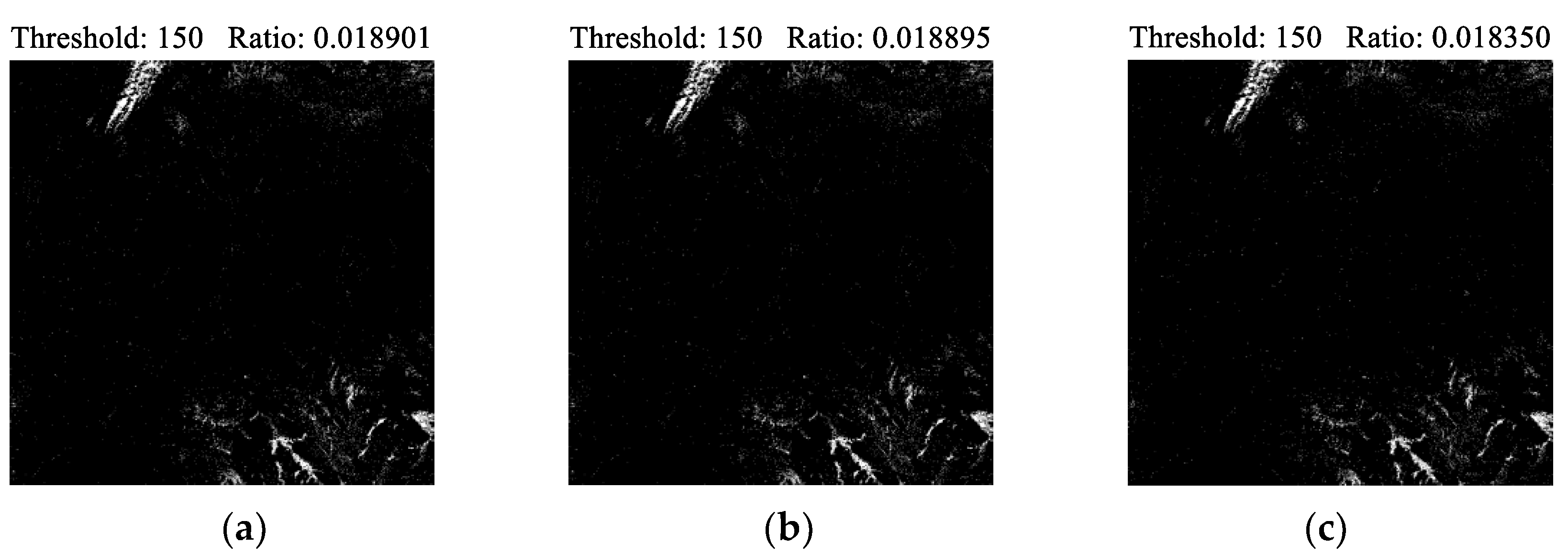
4.1. Comparison of Different Spatial Resolutions

As seen from

Table 7. Comparison of results from different spatial resolutions.

Dataset	P/%	R/%	mAP50/%
60 m	84.18	90.87	90.87
20 m	73.13	82.00	80.71
10 m	45.05	63.61	49.79

, the precision, recall, and mAP50 for the model were the highest when the red, green, and blue bands with a spatial resolution of 60 m were input into the model for training, with values of 84.18%, 90.87%, and 90.87%, respectively. The red, green, and blue bands with a spatial resolution of 10 m were input into the model for training, and the model had the lowest precision, recall, and mAP50, with values of 45.05%, 63.61%, and 49.79%, respectively. The precision, recall, and mAP50 of the model decrease with increasing spatial resolution.

The common understanding is that “the higher the spatial resolution, the higher the accuracy of remote sensing classification.” However, some studies are inconsistent with this finding. The effect of spatial resolution on satellite-based estimation of PM2.5 was analyzed by Bai et al. [55]. Their results showed that the summer AOD-PM2.5 correlation decreased from 0.42 to 0.49 when the spatial resolution decreased from 3 km to 10 km. They considered that part of the reason for this spatial resolution effect was that a coarser AOD resolution could better capture the spatial variability of PM2.5 in summer. Zheng et al. [56] estimated the PM2.5 levels using convolutional neural networks and random forest methods and also compared the prediction accuracy at different spatial resolutions (i.e., 670, 500, 200, and 100 m). It was found that the performance started to improve with increasing spatial resolution until a maximum response was realized at 200 m, after which the performance decreased. The results in Bai et al. [55] and Zheng et al. [56] indicated that the performance of the model does not necessarily improve but may decrease as the spatial resolution increases.

As the spatial resolution increases from 60 m to 10 m, the performance of the model gradually decreases. This effect may be due to the decrease in the model’s receptive field and the increase in noise. The clarity of the smoke outline and the purity of the pixels are generally positively correlated with the spatial resolution of remote sensing images. However, increasing the spatial resolution can also magnify the details of the smoke background, adding some interference noise to the remote sensing recognition and information extraction of smoke, thus reducing the performance of the model [57].

To verify the point above, binarization [58] was used to threshold segment images with different spatial resolutions. Image binarization first requires converting the image to grayscale. Then it classifies all pixels in an image based on their grayscale values. Pixels with grayscale values greater than or equal to a specified threshold are considered the object and assigned a value of 255, while pixels with grayscale values less than the threshold are considered the background and assigned a value of 0. By selecting an appropriate threshold, a binary image can be obtained that reflects the overall and local features of the original image. As can be seen from Figure 9, when the threshold value is 150, the smoke in the image acquired on 11 November 2020 was accurately segmented. However, there were also some instances of incorrect segmentation.

Figure 10 displays the outcomes of the segmentation process performed on images with varying spatial resolutions. Figure 10 also includes the calculation of the proportion of pixels in the entire image that were segmented as smoke.

From Figure 10, it is evident that in the image segmentation results with a spatial resolution of 10m, the proportion of pixels segmented as smoke (smoke pixels + noise) is the highest, accounting for 1.89% of the entire image. It is evident from Figure 10 that there is more noise in Figure 10a than in Figure 10b. Figure 10c shows the least amount of noise. This indicates that as the spatial resolution increases, there is a corresponding increase in noise, which has a more significant impact on the segmentation results.

4.2. The Challenge of Insufficient Data

Deep learning models often have deep and complex structures and require considerable training data [59]. However, the number of matched samples in remote sensing datasets is usually limited. This limitation can be attributed to many factors, such as the unavailability of satellite data due to large amounts of cloud cover [60]. Moreover, the morphology, movement, and other characteristics of the smoke produced by diverse scenarios vary [61]. Existing publicly available datasets contain minimal scenarios of smoke data, which leads to a lack of ability to adapt the smoke detection models to realistic scenarios. Furthermore, in the case of remote sensing data, there are currently no publicly available datasets of smoke from the burning of straw.

Because the smoke from burning straw is relatively delicate and readily obscured by clouds, only some high-quality images meet the aforementioned requirements. This study selected four scenes of remote sensing data containing smoke from straw burning. A smoke dataset of straw burning was constructed through data processing, including band synthesis, cropping, annotation, and data enhancement of the remote sensing images. As a result of training, improving the model, and adding input bands, the final accuracy reached 82.90%. However, the data for this study need to be larger than those of other publicly available datasets. The problem of insufficient data can be improved using migration learning [62]. Techniques and strategies in migration learning, such as pre-training, fine-tuning, and domain adaptation, are beneficial in solving the problem of insufficient data. Parameters in the models pre-trained on large datasets can be fine-tuned using a limited number of samples to achieve optimal performance in the new tasks [63].

In our next research study, we will use the data-based migration learning method. This approach solves the problem of model generalization between multiple sensor images. The land classification methods by Huang et al. [64] and Tong et al. [65] used data-based migration learning to improve the performance of the model when applied to multi-sensor images. The data used in this study are Sentinel-2 remote sensing data, and the model may need to be more effectively applied to other sensor images. Therefore, data-based migration learning techniques can be used to solve the problems of not having enough data and the model generalization issue among multiple sensor images.

4.3. Impact of Other Types of Smoke

In the present study, the pixels in the dataset that signified smoke were derived from the burning of straw. However, it was noticed that the areas around the arable land sometimes contained housing and factories. The burning of wood and coal also releases smoke, which can impact the detection results for smoke from straw burning. Chen et al. [3] differentiated biomass burning into four types: forest fires, open burning of agricultural straw, combustion of wood and straw as fuel, and miscellaneous sources. Chen et al. [3] analyzed several factors to distinguish between the four categories of biomass burning. The factors included the number of particles generated during combustion, emission factors, size distribution, and inventories of trace gas emissions.

In the future, we will consider adding fire point information, which combines wind speed, wind direction, humidity [66], and fire points to determine the source of the smoke. These different scenarios will produce smoke with different characteristics, such as differences in morphology, direction of movement, size distribution, and trace gas emission inventories [61]. Depending on the source of the smoke, we can classify it into three categories: smoke from straw burning, smoke from household burning, and smoke emitted by factories. The ability of the model to identify smoke from straw burning is improved by having the model learn the characteristics of other types of smoke to reduce their interference.

4.4. Real-Time Monitoring Issues

Satellite remote sensing technology has an extensive detection range and synchronous and economical monitoring capabilities. It can realize global observation of the Earth’s surface and provides a large amount of useful data and information for detecting smoke released from straw burning [67]. However, individual satellites are limited by their revisit times [68], such that they may not enable real-time monitoring of straw burning events. With the development of remote sensing technology, remote sensing images can now be obtained by multiple remote sensors that form clusters for all-around ground photography. The image data thus obtained contains high-precision surface information over a large area and within a shorter period, making real-time smoke monitoring possible [69]. In future research, we will combine our model with remote sensing images acquired by multiple satellite sensors and geostationary satellites to identify the smoke produced by straw burning and target the approximate area of straw burning. Unmanned aerial vehicles (UAVs) will also be used to conduct accurate monitoring in selected areas. Multi-source data fusion will be used to solve the real-time problem of satellite remote-sensing smoke detection.

5. Conclusions

Burning straw is very destructive, threatens people’s livelihoods and property, and causes irreparable environmental damage. As one of the most significant features of straw burning, smoke is used to detect the occurrence of straw burning. In this study, different input combinations of Sentinel-2 data bands were analyzed, and the band combined with the highest detection accuracy was the RGB_Band6, with an accuracy rate of 82.90%. The SE network attention mechanism was introduced based on the YOLOv5s model so that the delicate features of the smoke were enhanced. The Mish activation function replaced the Leaky ReLU activation function. The accuracy of the improved model was 75.63%, which was 1.81% better than before the improvement. We also analyzed the effect of spatial resolution on model detection, and accuracy rates of 84.18%, 73.13%, and 45.05% for images of 60-, 20-, and 10-m resolution, respectively, were achieved. Our experiments showed that the model accuracy only sometimes improves with increasing spatial resolution. Problems such as insufficient data will be addressed in future research using migration learning and data fusion from multiple sources. The improved method proposed in this study can accurately identify smoke and provide a methodological reference for improving smoke detection and effective control of straw burning.

References

1. Akagi, S.K.; Yokelson, R.J.; Wiedinmyer, C.; Alvarado, M.J.; Reid, J.S.; Karl, T.; Crounse, J.D.; Wennberg, P.O. Emission Factors for Open and Domestic Biomass Burning for Use in Atmospheric Models. Atmos. Chem. Phys. 2011, 11, 4039–4072. [Google Scholar] [CrossRef]
2. van Marle, M.J.; Kloster, S.; Magi, B.I.; Marlon, J.R.; Daniau, A.-L.; Field, R.D.; Arneth, A.; Forrest, M.; Hantson, S.; Kehrwald, N.M.; et al. Historic Global Biomass Burning Emissions for CMIP6 (BB4CMIP) Based on Merging Satellite Observations with Proxies and Fire Models (1750–2015). Geosci. Model Dev. 2017, 10, 3329–3357. [Google Scholar] [CrossRef]
3. Chen, J.; Li, C.; Ristovski, Z.; Milic, A.; Gu, Y.; Islam, M.S.; Wang, S.; Hao, J.; Zhang, H.; He, C.; et al. A Review of Biomass Burning: Emissions and Impacts on Air Quality, Health and Climate in China. Sci. Total Environ. 2017, 579, 1000–1034. [Google Scholar] [CrossRef]
4. Shi, Z.; Yang, S.; Chang, Z.; Zhang, S. Investigation of Straw Yield and Utilization Status and Analysis of Difficulty in Prohibition Straw Burning: A Case Study in A Township in Jiangsu Province, China. J. Agric. Resour. Environ. 2014, 31, 103. [Google Scholar]
5. Mehmood, K.; Chang, S.; Yu, S.; Wang, L.; Li, P.; Li, Z.; Liu, W.; Rosenfeld, D.; Seinfeld, J.H. Spatial and Temporal Distributions of Air Pollutant Emissions from Open Crop Straw and Biomass Burnings in China from 2002 to 2016. Environ. Chem. Lett. 2018, 16, 301–309. [Google Scholar] [CrossRef]
6. Yim, H.; Oh, S.; Kim, W. A Study on the Verification Scheme for Electrical Circuit Analysis of Fire Hazard Analysis in Nuclear Power Plant. J. Korean Soc. Saf. 2015, 30, 114–122. [Google Scholar] [CrossRef]
7. Mehmood, K.; Bao, Y.; Saifullah; Bibi, S.; Dahlawi, S.; Yaseen, M.; Abrar, M.M.; Srivastava, P.; Fahad, S.; Faraj, T.K. Contributions of Open Biomass Burning and Crop Straw Burning to Air Quality: Current Research Paradigm and Future Outlooks. Front. Environ. Sci. 2022, 10, 852492. [Google Scholar] [CrossRef]
8. Xiaohui, M.; Yixi, T.; Zhaobin, S.; Ziming, L. Analysis on the Impacts of Straw Burning on Air Quality in Beijing-Tianjing-Hebei Region. Meteorol. Environ. Res. 2017, 8, 49–53. [Google Scholar]
9. Mott, J.A.; Meyer, P.; Mannino, D.; Redd, S.C.; Smith, E.M.; Gotway-Crawford, C.; Chase, E. Wildland Forest Fire Smoke: Health Effects and Intervention Evaluation, Hoopa, California, 1999. West. J. Med. 2002, 176, 157. [Google Scholar] [CrossRef]
10. Hasinoff, S.W.; Kutulakos, K.N. Photo-Consistent Reconstruction of Semitransparent Scenes by Density-Sheet Decomposition. IEEE Trans. Pattern Anal. Mach. Intell. 2007, 29, 870–885. [Google Scholar] [CrossRef]
11. Jiang, M.; Zhao, Y.; Yu, F.; Zhou, C.; Peng, T. A self-attention network for smoke detection. Fire Saf. J. 2022, 129, 103547. [Google Scholar] [CrossRef]
12. Avgeris, M.; Spatharakis, D.; Dechouniotis, D.; Kalatzis, N.; Roussaki, I.; Papavassiliou, S. Where There Is Fire There Is Smoke: A Scalable Edge Computing Framework for Early Fire Detection. Sensors 2019, 19, 639. [Google Scholar] [CrossRef] [PubMed]
13. Tlig, L.; Bouchouicha, M.; Tlig, M.; Sayadi, M.; Moreau, E. A Fast Segmentation Method for Fire Forest Images Based on Multiscale Transform and PCA. Sensors 2020, 20, 6429. [Google Scholar] [CrossRef]
14. Yoon, J.H.; Kim, S.-M.; Eom, Y.; Koo, J.M.; Cho, H.-W.; Lee, T.J.; Lee, K.G.; Park, H.J.; Kim, Y.K.; Yoo, H.-J.; et al. Extremely Fast Self-Healable Bio-Based Supramolecular Polymer for Wearable Real-Time Sweat-Monitoring Sensor. ACS Appl. Mater. Interfaces 2019, 11, 46165–46175. [Google Scholar] [CrossRef]
15. Deng, C.; Ji, X.; Rainey, C.; Zhang, J.; Lu, W. Integrating Machine Learning with Human Knowledge. iScience 2020, 23, 101656. [Google Scholar] [CrossRef] [PubMed]
16. Nie, S.; Zhang, Y.; Wang, L.; Wu, Q.; Wang, S. Preparation and Characterization of Nanocomposite Films Containing Nano-Aluminum Nitride and Cellulose Nanofibrils. Nanomaterials 2019, 9, 1121. [Google Scholar] [CrossRef]
17. Liu, K.; Li, Y.; Han, T.; Yu, X.; Ye, H.; Hu, H.; Hu, Z. Evaluation of Grain Yield Based on Digital Images of Rice Canopy. Plant Methods 2019, 15, 28. [Google Scholar] [CrossRef]
18. Gubbi, J.; Marusic, S.; Palaniswami, M. Smoke Detection in Video Using Wavelets and Support Vector Machines. Fire Saf. J. 2009, 44, 1110–1115. [Google Scholar] [CrossRef]
19. Chen, T.-H.; Wu, P.-H.; Chiou, Y.-C. An Early Fire-Detection Method Based on Image Processing. In Proceedings of the 2004 International Conference on Image Processing (ICIP’04), Singapore, 24–27 October 2004; IEEE: Piscataway, NJ, USA, 2004; Volume 3, pp. 1707–1710. [Google Scholar]
20. Li, H.; Yuan, F. Image Based Smoke Detection Using Pyramid Texture and Edge Features. J. Image Graph. 2015, 20, 0772–0780. [Google Scholar]
21. Xie, Y.; Qu, J.; Xiong, X.; Hao, X.; Che, N.; Sommers, W. Smoke Plume Detection in the Eastern United States Using MODIS. Int. J. Remote Sens. 2007, 28, 2367–2374. [Google Scholar] [CrossRef]
22. Zhao, T.X.-P.; Ackerman, S.; Guo, W. Dust and Smoke Detection for Multi-Channel Imagers. Remote Sens. 2010, 2, 2347–2368. [Google Scholar] [CrossRef]
23. Li, Z.; Khananian, A.; Fraser, R.H.; Cihlar, J. Automatic Detection of Fire Smoke Using Artificial Neural Networks and Threshold Approaches Applied to AVHRR Imagery. IEEE Trans. Geosci. Remote Sens. 2001, 39, 1859–1870. [Google Scholar] [CrossRef]
24. Redmon, J.; Divvala, S.; Girshick, R.; Farhadi, A. You Only Look Once: Unified, Real-Time Object Detection. In Proceedings of the IEEE Conference on Computer Vision and Pattern Recognition, Las Vegas, NV, USA, 26 June–1 July 2016; pp. 779–788. [Google Scholar]
25. Yan, B.; Fan, P.; Lei, X.; Liu, Z.; Yang, F. A Real-Time Apple Targets Detection Method for Picking Robot Based on Improved YOLOv5. Remote Sens. 2021, 13, 1619. [Google Scholar] [CrossRef]
26. Drusch, M.; Del Bello, U.; Carlier, S.; Colin, O.; Fernandez, V.; Gascon, F.; Hoersch, B.; Isola, C.; Laberinti, P.; Martimort, P.; et al. Sentinel-2: ESA’s Optical High-Resolution Mission for GMES Operational Services. Remote Sens. Environ. 2012, 120, 25–36. [Google Scholar] [CrossRef]
27. Hu, J.; Shen, L.; Sun, G. Squeeze-and-Excitation Networks. In Proceedings of the IEEE Conference on Computer Vision and Pattern Recognition, Salt Lake City, UT, USA, 18–23 June 2018; pp. 7132–7141. [Google Scholar]
28. Misra, D. Mish: A Self Regularized Non-Monotonic Neural Activation Function. arXiv 2019, arXiv:1908.08681. [Google Scholar]
29. Yan, L.; Wang, Y.; Feng, G.; Gao, Q. Status and Change Characteristics of Farmland Soil Fertility in Jilin Province. Sci. Agric. Sin. 2015, 48, 4800–4810. [Google Scholar]
30. Liu, H.; Li, J.; Du, J.; Zhao, B.; Hu, Y.; Li, D.; Yu, W. Identification of Smoke from Straw Burning in Remote Sensing Images with the Improved YOLOv5s Algorithm. Atmosphere 2022, 13, 925. [Google Scholar] [CrossRef]
31. Xi, W.; Sun, Y.; Yu, G.; Zhang, Y. The Research About the Effect of Straw Resources on the Economic Structure of Jilin Province. In Proceedings of the 22nd International Conference on Industrial Engineering and Engineering Management 2015; Springer: Berlin/Heidelberg, Germany, 2016; pp. 511–518. [Google Scholar]
32. Guo, H.; Xu, S.; Wang, X.; Shu, W.; Chen, J.; Pan, C.; Guo, C. Driving Mechanism of Farmers’ Utilization Behaviors of Straw Resources—An Empirical Study in Jilin Province, the Main Grain Producing Region in the Northeast Part of China. Sustainability 2021, 13, 2506. [Google Scholar] [CrossRef]
33. Wang, X.; Wang, X.; Geng, P.; Yang, Q.; Chen, K.; Liu, N.; Fan, Y.; Zhan, X.; Han, X. Effects of Different Returning Method Combined with Decomposer on Decomposition of Organic Components of Straw and Soil Fertility. Sci. Rep. 2021, 11, 15495. [Google Scholar] [CrossRef]
34. Huo, Y.; Li, M.; Teng, Z.; Jiang, M. Analysis on Effect of Straw Burning on Air Quality in Harbin. Environ. Pollut. Control 2018, 40, 1161–1166. [Google Scholar]
35. Wang, J.; Xie, X.; Fang, C. Temporal and Spatial Distribution Characteristics of Atmospheric Particulate Matter (PM10 and PM2.5) in Changchun and Analysis of Its Influencing Factors. Atmosphere 2019, 10, 651. [Google Scholar] [CrossRef]
36. Li, J.; Roy, D.P. A Global Analysis of Sentinel-2A, Sentinel-2B and Landsat-8 Data Revisit Intervals and Implications for Terrestrial Monitoring. Remote Sens. 2017, 9, 902. [Google Scholar] [CrossRef]
37. Louis, J.; Debaecker, V.; Pflug, B.; Main-Knorn, M.; Bieniarz, J.; Mueller-Wilm, U.; Cadau, E.; Gascon, F. Sentinel-2 Sen2Cor: L2A Processor for Users. In Proceedings of the Proceedings Living Planet Symposium, Prague, Czech Republic, 9–13 May 2016; pp. 1–8. [Google Scholar]
38. Johnson, A.D.; Handsaker, R.E.; Pulit, S.L.; Nizzari, M.M.; O’Donnell, C.J.; de Bakker, P.I. SNAP: A Web-Based Tool for Identification and Annotation of Proxy SNPs Using HapMap. Bioinformatics 2008, 24, 2938–2939. [Google Scholar] [CrossRef] [PubMed]
39. Juan, Y.; Shun, L. Detection Method of Illegal Building Based on YOLOv5. Comput. Eng. Appl. 2021, 57, 236–244. [Google Scholar]
40. Ting, L.; Baijun, Z.; Yongsheng, Z.; Shun, Y. Ship Detection Algorithm Based on Improved YOLO V5. In Proceedings of the 2021 6th International Conference on Automation, Control and Robotics Engineering (CACRE), Dalian, China, 15–17 July 2021; IEEE: Piscataway, NJ, USA, 2021; pp. 483–487. [Google Scholar]
41. Lin, T.-Y.; Dollár, P.; Girshick, R.; He, K.; Hariharan, B.; Belongie, S. Feature Pyramid Networks for Object Detection. In Proceedings of the IEEE Conference on Computer Vision and Pattern Recognition, Honolulu, HI, USA, 21–26 July 2017; pp. 2117–2125. [Google Scholar]
42. Liu, S.; Qi, L.; Qin, H.; Shi, J.; Jia, J. Path Aggregation Network for Instance Segmentation. In Proceedings of the IEEE Conference on Computer Vision and Pattern Recognition, Salt Lake City, UT, USA, 18–23 June 2018; pp. 8759–8768. [Google Scholar]
43. Wang, Y.; Ma, H.; Alifu, K.; Lv, Y. Remote Sensing Image Description Based on Word Embedding and End-to-End Deep Learning. Sci. Rep. 2021, 11, 3162. [Google Scholar] [CrossRef]
44. Song, Z.; Zhang, Z.; Yang, S.; Ding, D.; Ning, J. Identifying Sunflower Lodging Based on Image Fusion and Deep Semantic Segmentation with UAV Remote Sensing Imaging. Comput. Electron. Agric. 2020, 179, 105812. [Google Scholar] [CrossRef]
45. Qiu, C.; Zhang, S.; Wang, C.; Yu, Z.; Zheng, H.; Zheng, B. Improving Transfer Learning and Squeeze- and-Excitation Networks for Small-Scale Fine-Grained Fish Image Classification. IEEE Access 2018, 6, 78503–78512. [Google Scholar] [CrossRef]
46. Maas, A.L.; Hannun, A.Y.; Ng, A.Y. Rectifier Nonlinearities Improve Neural Network Acoustic Models. In Proceedings of the 30th International Conference on Machine Learning, ICML 2013, Atlanta, GA, USA, 16–21 June 2013; Volume 30, p. 3. [Google Scholar]
47. Rahman, M.A.; Wang, Y. Optimizing Intersection-over-Union in Deep Neural Networks for Image Segmentation. In Proceedings of the International Symposium on Visual Computing, Las Vegas, NV, USA, 12–14 December 2016; Springer: Berlin/Heidelberg, Germany, 2016; pp. 234–244. [Google Scholar]
48. Zhou, L.; Li, Y.; Rao, X.; Liu, C.; Zuo, X.; Liu, Y. Ship Target Detection in Optical Remote Sensing Images Based on Multiscale Feature Enhancement. Comput. Intell. Neurosci. 2022, 2022, 2605140. [Google Scholar] [CrossRef]
49. John, P.S.; Bomble, Y.J. Approaches to Computational Strain Design in the Multiomics Era. Front. Microbiol. 2019, 10, 597. [Google Scholar] [CrossRef]
50. Li, X.; Song, W.; Lian, L.; Wei, X. Forest Fire Smoke Detection Using Back-Propagation Neural Network Based on MODIS Data. Remote Sens. 2015, 7, 4473–4498. [Google Scholar] [CrossRef]
51. Li, X.; Wang, J.; Song, W.; Ma, J.; Telesca, L.; Zhang, Y. Automatic Smoke Detection in Modis Satellite Data Based on K-Means Clustering and Fisher Linear Discrimination. Photogramm. Eng. Remote Sens. 2014, 80, 971–982. [Google Scholar] [CrossRef]
52. Woo, S.; Park, J.; Lee, J.-Y.; Kweon, I.S. Cbam: Convolutional Block Attention Module. In Proceedings of the European Conference on Computer Vision (ECCV), Munich, Germany, 8–14 September 2018; pp. 3–19. [Google Scholar]
53. Xiang, X.; Du, J.; Jacinthe, P.-A.; Zhao, B.; Zhou, H.; Liu, H.; Song, K. Integration of Tillage Indices and Textural Features of Sentinel-2A Multispectral Images for Maize Residue Cover Estimation. Soil Tillage Res. 2022, 221, 105405. [Google Scholar] [CrossRef]
54. Wang, Z.; Yang, P.; Liang, H.; Zheng, C.; Yin, J.; Tian, Y.; Cui, W. Semantic Segmentation and Analysis on Sensitive Parameters of Forest Fire Smoke Using Smoke-Unet and Landsat-8 Imagery. Remote Sens. 2022, 14, 45. [Google Scholar] [CrossRef]
55. Bai, H.; Shi, Y.; Seong, M.; Gao, W.; Li, Y. Influence of Spatial Resolution on Satellite-Based PM2.5 Estimation: Implications for Health Assessment. Remote Sens. 2022, 14, 2933. [Google Scholar] [CrossRef]
56. Zheng, T.; Bergin, M.H.; Hu, S.; Miller, J.; Carlson, D.E. Estimating Ground-Level PM2.5 Using Micro-Satellite Images by a Convolutional Neural Network and Random Forest Approach. Atmos. Environ. 2020, 230, 117451. [Google Scholar] [CrossRef]
57. Wang, Q.; Xu, J.; Chen, Y.; Li, J.; Wang, X. Influence of the Varied Spatial Resolution of Remote Sensing Images on Urban and Rural Residential Information Extraction. Resour. Sci. 2012, 34, 159–165. (In Chinese) [Google Scholar]
58. Otsu, N. A threshold Selection Method from Gray-Level Histograms. IEEE Trans. Syst. Man Cybern. 1979, 9, 62–66. [Google Scholar] [CrossRef]
59. Huang, S.; Yang, J.; Fong, S.; Zhao, Q. Artificial Intelligence in Cancer Diagnosis and Prognosis: Opportunities and Challenges. Cancer Lett. 2020, 471, 61–71. [Google Scholar] [CrossRef]
60. Han, L.; Yang, G.; Dai, H.; Xu, B.; Yang, H.; Feng, H.; Li, Z.; Yang, X. Modeling Maize Above-Ground Biomass Based on Machine Learning Approaches Using UAV Remote-Sensing Data. Plant Methods 2019, 15, 10. [Google Scholar] [CrossRef]
61. Shamjad, P.; Tripathi, S.; Pathak, R.; Hallquist, M.; Arola, A.; Bergin, M. Contribution of Brown Carbon to Direct Radiative Forcing over the Indo-Gangetic Plain. Environ. Sci. Technol. 2015, 49, 10474–10481. [Google Scholar] [CrossRef]
62. Goodfellow, I.; Bengio, Y.; Courville, A. Deep Learning; MIT Press: Cambridge, MA, USA, 2016. [Google Scholar]
63. Yuan, Q.; Shen, H.; Li, T.; Li, Z.; Li, S.; Jiang, Y.; Xu, H.; Tan, W.; Yang, Q.; Wang, J.; et al. Deep Learning in Environmental Remote Sensing: Achievements and Challenges. Remote Sens. Environ. 2020, 241, 111716. [Google Scholar] [CrossRef]
64. Huang, B.; Zhao, B.; Song, Y. Urban land-Use Mapping Using a Deep Convolutional Neural Network with High Spatial Resolution Multispectral Remote Sensing Imagery. Remote Sens. Environ. 2018, 214, 73–86. [Google Scholar] [CrossRef]
65. Tong, X.-Y.; Xia, G.-S.; Lu, Q.; Shen, H.; Li, S.; You, S.; Zhang, L. Land-Cover Classification with High-Resolution Remote Sensing Images Using Transferable Deep Models. Remote Sens. Environ. 2020, 237, 111322. [Google Scholar] [CrossRef]
66. Li, Y.; Zheng, C.; Ma, Z.; Quan, W. Acute and Cumulative Effects of Haze Fine Particles on Mortality and the Seasonal Characteristics in Beijing, China, 2005–2013: A Time-Stratified Case-Crossover Study. Int. J. Environ. Res. Public Health 2019, 16, 2383. [Google Scholar] [CrossRef]
67. Cao, H.; Han, L. The Short-Term Impact of the COVID-19 Epidemic on Socioeconomic Activities in China Based on the OMI-NO2 Data. Environ. Sci. Pollut. Res. 2022, 29, 21682–21691. [Google Scholar] [CrossRef]
68. Kumar, D. Urban Objects Detection from C-Band Synthetic Aperture Radar (SAR) Satellite Images through Simulating Filter Properties. Sci. Rep. 2021, 11, 6241. [Google Scholar] [CrossRef]
69. Wang, J.; Xiao, X.; Qin, Y.; Dong, J.; Zhang, G.; Kou, W.; Jin, C.; Zhou, Y.; Zhang, Y. Mapping Paddy Rice Planting Area in Wheat-Rice Double-Cropped Areas through Integration of Landsat-8 OLI, MODIS and PALSAR images. Sci. Rep. 2015, 5, 10088. [Google Scholar] [CrossRef]
Figure 1. Diagram of the study area.
Remotesensing 15 02641 g001
Figure 2. Schematic diagram of the temporal and spatial distribution of the Sentinel-2 image.
Remotesensing 15 02641 g002
Figure 3. Typical examples of smoke used for model training.
Remotesensing 15 02641 g003
Figure 4. A smoke image for straw burning with different image enhancements. (a) is the original image; (b) is pan + change brightness + add noise; (c) is rotate + change brightness + mirror; (d) is pan + change brightness; (e) is change brightness + mirror; and (f) is pan + add noise + cutout + change brightness.
Remotesensing 15 02641 g004
Figure 5. Improved YOLOv5s structure diagram. Note: CBM is Convolution + Batch normalization + Mish; CSP is cross-stage partial connections; SESPP is Squeeze-and-Excitation network + Spatial Pyramid Pooling module; and Conv is Convolution module.
Remotesensing 15 02641 g005
Figure 6. Areas of sample cell points extracted for spectral analysis: (a) 4, 3, and 2-band synthesis of Sentinel-2 images from central Jilin Province, China, on 14 November 2020; (b) classified images (red for smoke cells, light blue for cloud cells, yellow for background cells, and dark blue for water cells).
Remotesensing 15 02641 g006
Figure 7. Spectral response curves for the four feature types in bands 1–8A.
Remotesensing 15 02641 g007
Figure 8. H values for the three different pairs of features (smoke vs. clouds, smoke vs. background, and smoke vs. water).
Remotesensing 15 02641 g008
Figure 9. Binarization segmentation results for the 11 November 2020 image at different thresholds.
Remotesensing 15 02641 g009
Figure 10. Binarization segmentation results for different spatial resolutions at a threshold of 150: (a) spatial resolution is 10 m; (b) spatial resolution is 20 m; and (c) spatial resolution is 60 m.
Remotesensing 15 02641 g010