Article

Deep Learning of High-Resolution Unmanned Aerial Vehicle Imagery for Classifying Halophyte Species: A Comparative Study for Small Patches and Mixed Vegetation

1
Korea Ocean Satellite Center, Korea Institute of Ocean Science and Technology, Busan 49111, Republic of Korea
2
Ocean Climate Response & Ecosystem Report Department, Korea Institute of Ocean Science and Technology, Busan 49111, Republic of Korea
*
Author to whom correspondence should be addressed.
Remote Sens. 2023, 15(11), 2723; https://doi.org/10.3390/rs15112723
Submission received: 26 April 2023 / Revised: 18 May 2023 / Accepted: 22 May 2023 / Published: 24 May 2023
(This article belongs to the Section Remote Sensing in Agriculture and Vegetation)

Abstract

:
Recent advances in deep learning (DL) and unmanned aerial vehicle (UAV) technologies have made it possible to monitor salt marshes more efficiently and precisely. However, studies have rarely compared the classification performance of DL with the pixel-based method for coastal wetland monitoring using UAV data. In particular, many studies have been conducted at the landscape level; however, little is known about the performance of species discrimination in very small patches and in mixed vegetation. We constructed a dataset based on UAV-RGB data and compared the performance of pixel-based and DL methods for five scenarios (combinations of annotation type and patch size) in the classification of salt marsh vegetation. Maximum likelihood, a pixel-based classification method, showed the lowest overall accuracy of 73%, whereas the U-Net classification method achieved over 90% accuracy in all classification scenarios. As expected, in a comparison of pixel-based and DL methods, the DL approach achieved the most accurate classification results. Unexpectedly, there was no significant difference in overall accuracy between the two annotation types and labeling data sizes in this study. However, when comparing the classification results in detail, we confirmed that polygon-type annotation was more effective for mixed-vegetation classification than the bounding-box type. Moreover, the smaller size of labeling data was more effective for detecting small vegetation patches. Our results suggest that a combination of UAV-RGB data and DL can facilitate the accurate mapping of coastal salt marsh vegetation at the local scale.

Graphical Abstract

1. Introduction

Coastal salt marshes are wetland ecosystems at the land-sea boundary that play important roles in ecological and anthropogenic processes [1]. Salt marshes have various ecological functions, offering barriers against storm surges, the means for purifying pollutants and sequestering carbon, water-quality enhancement, and suitable habitats for benthic fauna [2,3,4]. It is known that coastal wetlands are gradually decreasing due to anthropogenic modification and global change, including reclamation, barriers, tourism infrastructure, overgrazing, alien species invasion, and sea level rise [5,6,7]. Therefore, monitoring and managing coastal wetland ecosystems in a non-destructive manner is becoming an urgent task.
The monitoring of coastal salt marshes can be restricted due to the time limitation for surveying as a result of periodic flooding and physical difficulties with muddy environments [8,9]. Therefore, the field surveying method and passive satellite remote-sensing techniques are limited in their ability to fully investigate salt marshes [10,11]. At the local scale, the use of unmanned aerial vehicles (UAVs) is an emerging technology in conducting active remote-sensing surveys. Advances in UAV technology have been applied to vegetation mapping of wetlands [12], monitoring invasive species [13], and estimating aboveground biomass [14]; for instance, UAVs have gradually become an essential tool for coastal vegetation mapping.
The classification of salt marsh vegetation from remote sensing data is usually performed using pixel-based and object-based image analysis (OBIA) classification. For example, researchers [15] tested the accuracy of image classification using multi-spectral aerial photography. The accuracy of the unsupervised classification method achieved in this simplified model was only moderate. Other researchers [16] used supervised classification techniques for mapping wild taro from an aerial photograph and obtained classification results with a high overall accuracy (OA) of 94%. Some studies have compared object-based and pixel-based classification techniques [17,18]. For instance, one study [17] examined object-based classification methods for UAV images of wetland vegetation and compared their performance with pixel-based classification approaches; object-based classification provided higher accuracy than pixel-based classification when the same type of classifier was used.
Several studies have shown that the accuracy of remote sensing classification can be improved as the spatial resolution increases in remote-sensing monitoring of coastal wetlands [19,20]. However, the high spatial resolution of UAV images reduced the accuracy of the classification results, especially in wetlands vegetation [21]. Therefore, multiband and hyperspectral images are used for this purpose instead of red–green–blue (RGB) images due to the complex vegetation composition. In fact, hyperspectral images have been proven useful for classifying complex vegetation composition due to the advantages of using hundreds of narrow bands and a continuous spectral profile [22,23,24]. Nevertheless, UAV-RGB sensors are most commonly used for wetland vegetation classification [25,26]. Therefore, it is necessary to find a method that improves the accuracy of the vegetation classification results for wetland vegetation, in consideration of the limitations of the spectral information in UAV-RGB data.
Due to rapid technological developments, deep-learning (DL) technology is increasingly being applied in the processing of UAV data with excellent results [21,27]. Numerous studies have used this method for UAV-based mapping of coastal vegetation areas, often in comparison with conventional pixel-based methods [18,21]. In a comparison of the classification results of several traditional pixel-based and DL methods, the DL model achieved the best classification accuracy [21]. Moreover, after comparing machine-learning (ML) models (decision trees, support vector machine, k-nearest neighbor, and random forest) and DL models (convolution neural network, SegNet, U-Net, and PSPNet) in the classification of coastal wetland vegetation, the advantages of the DL model in the classification of UAV data were highlighted [27]. Many studies have demonstrated that both ML and DL can be applied to UAV image segmentation for improving the accuracy of classification [21,27]. However, to improve the classification performance based on DL, many variables must be considered, such as the selection of suitable models, the number of training datasets, the patch size of the input data, the filter size, the batch size, and the number of iterations. In other words, it is not clear which technique, i.e., traditional pixel-based classification or DL, is better for the classification of salt marsh vegetation.
Achieving accurate classification results in salt marsh environments is challenging, given the mixed dense vegetation. Moreover, if the same vegetation has different colors or different vegetation has similar morphological characteristics, classification becomes even more difficult. Therefore, in this study, we aimed to identify the more appropriate and accurate method for coastal salt marsh vegetation classification at the species level based on UAV-RGB imagery. The objectives of this study were to assess the DL classifiers using different training sample sizes and annotation types and then compare their performance with traditional pixel-based classification. In addition, we investigated the relative importance of features in the classification of coastal salt marsh vegetation using the DL method. The results of this study will provide insights into the techniques for the fine classification of complex vegetation and their applicability for future studies.

2. Materials and Methods
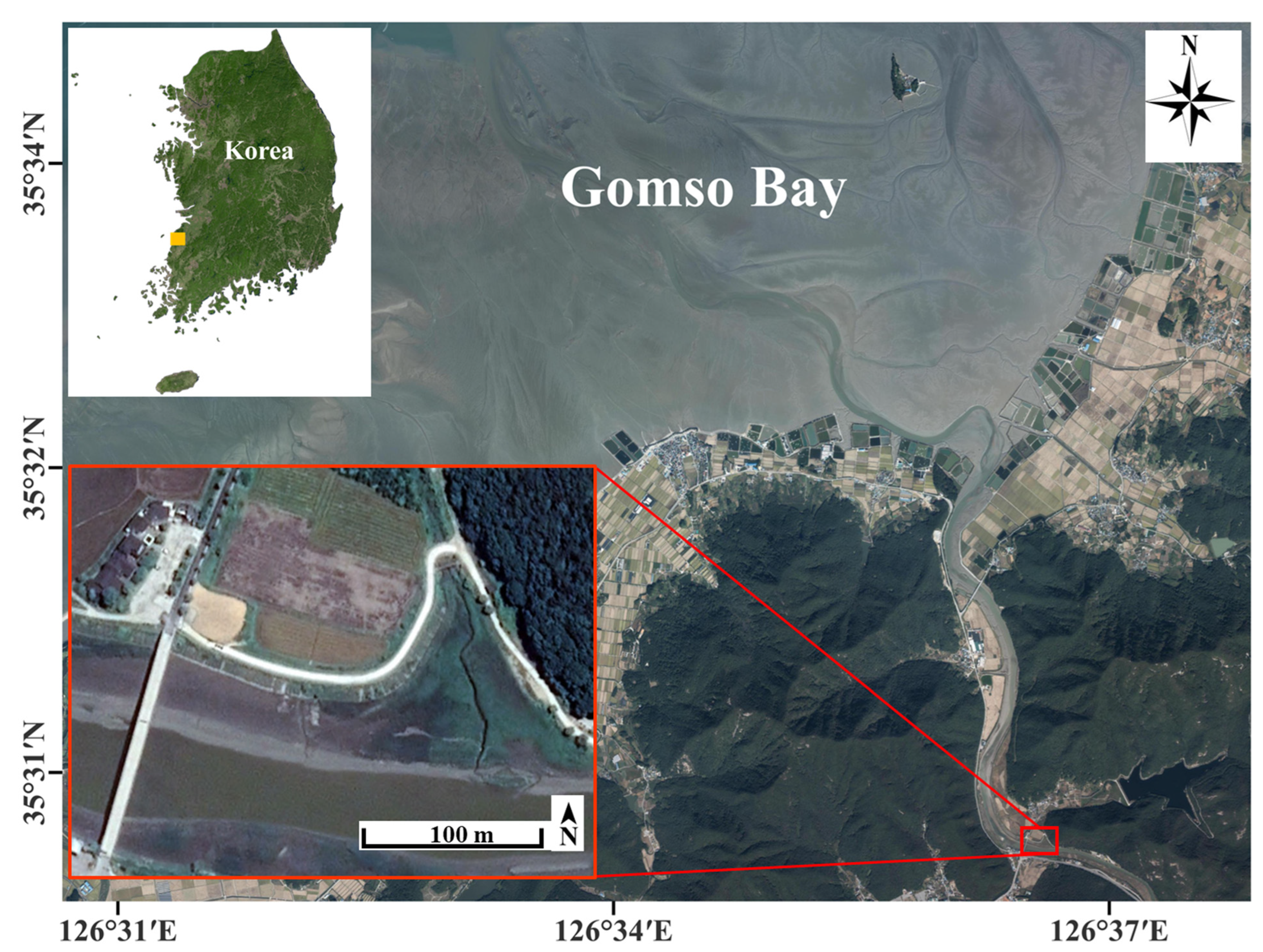
2.1. Study Area

The study area is located in the natural salt marshes of Jujin Estuary, central western coast, Korean Peninsula (Figure 1). The site is connected to Gomso Bay and is an important salt marsh for migratory waterbirds along the western coast of Korea. Gomso Bay is also a United Nations Educational, Scientific, and Cultural Organization World Natural Heritage site as of 2021. The study area is classified as a saltwater tidal marsh, which is influenced by the daily influx of tides. Generally, zonation in salt marshes is determined by abiotic factors such as salinity, tide elevation, soil moisture content, and local topography [28,29,30]. In the study area, this zonation of salt marsh vegetation is observed. Phragmites communis Trin. and Suaeda maritima (L.) Dumort are widely distributed, and P. communis and S. maritima are dominant in the eastern and western parts of the study area, respectively. The shoots of the halophyte S. maritima change in color between seasons, namely from green in spring to red-violet in late summer; this color change is salinity dependent [31]. In the study area, S. maritima gradually turns red as the altitude of the topography increases (Figure 2). Thus, this site was selected because the species present and their coverage allowed for the evaluation of the classification methods of fine and mixed vegetation.

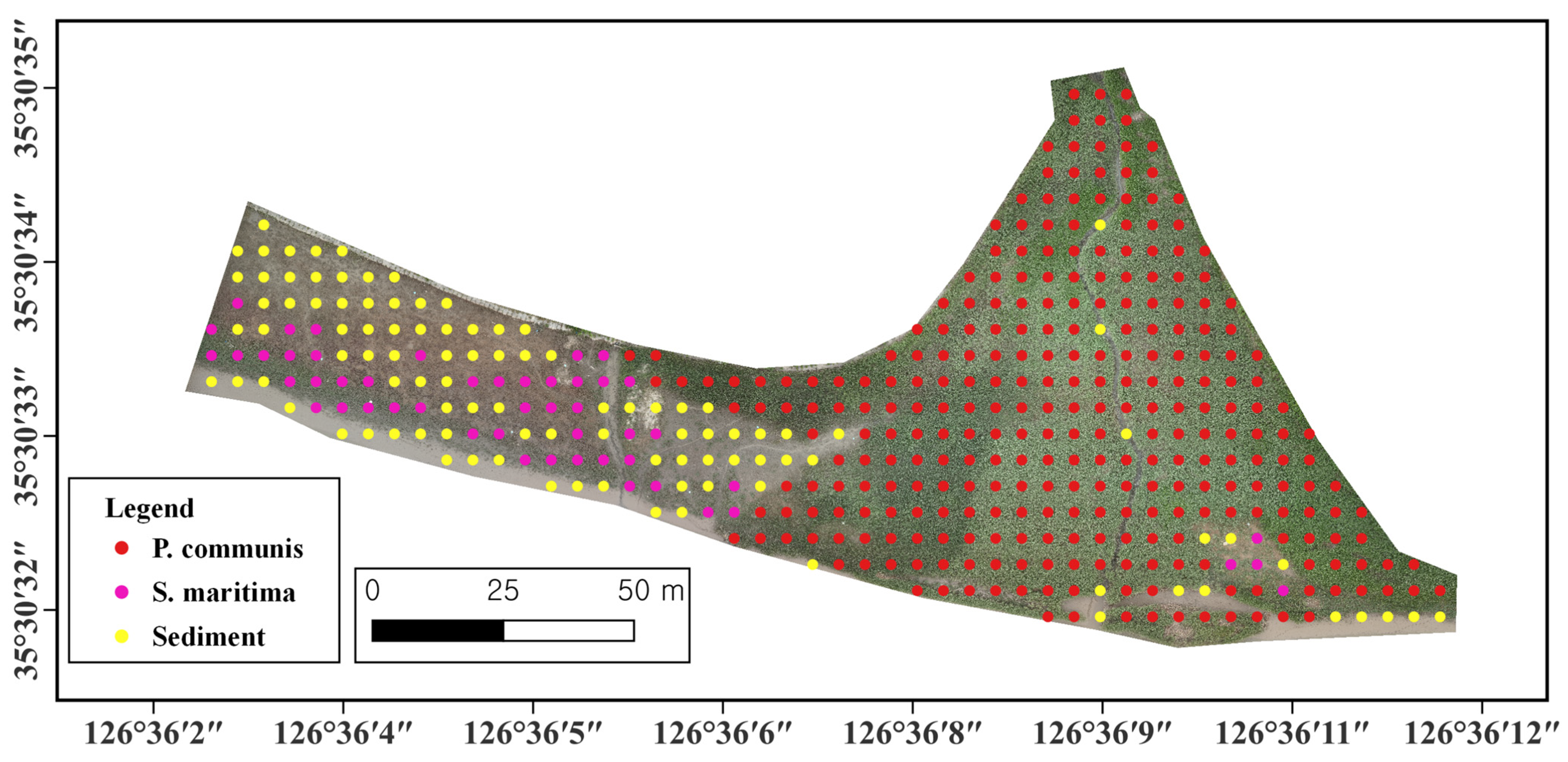
2.2. In-Situ Field Work and Unmanned Aerial Vehicle Image Acquisition

Photogrammetry images were acquired in Jujin Estuary from 24 June to 25 June 2021. In this study, a Matrice 300 RTK UAV with a Zenmuse P1 RGB sensor (35 mm fixed-focus lens; DJI, Nanshan, China) was used. The flight speed of the UAV was set to 10 m/s at 50 m of altitude. The overlap rate of the heading and side direction was set to 80%. For accurate georeferencing of UAV images, ten blue papers with black cross markers were used as ground control points (GCPs). After the UAV survey, the geolocation of GCPs was measured using a real-time kinematic (RTK) GPS (Leica GS16 antenna with CS20 3.75 G controller; Leica Geosystems, Heerbrug, Switzerland) with an RMSE of 0.015 m and 0.021 m for horizontal and vertical accuracy, respectively.
To better understand the spatial distribution of vegetation communities, we conducted a field survey of salt marsh vegetation groups in Jujin Estuary from 24 June to 25 June 2021. There are 108 field stations, used as calibration points in this investigation (Figure 2). These calibration points were also measured and surveyed with an RTK GPS. Additional information, such as plant species, height, and color, was also recorded. To secure more verification points, only vegetation patches that could be reliably identified in UAV images were digitized on the screen using an image analysis tool. The field-survey data were also used as a reference for selecting training and validation samples.

2.3. UAV Data Processing

The UAV-RGB image dataset was processed using Agisoft Metashape Professional software (version 1.8.2; Agisoft, St. Petersburg, Russia) to generate an orthomosaic photo. Image processing using the Metashape was performed in the following order: align photo, build dense point cloud, build mesh (3D polygonal model), build digital elevation model (DEM), and then build orthomosaic photo. To improve alignment results, the image quality value was set to 0.5 to exclude poorly focused images at the align-photo stage. Additionally, alignment parameters set the quality level at the highest, and the key point limit and tie point limit were set to 40,000 and 10,000, respectively. After alignment, a dense point cloud was generated based on the position (latitude and longitude) and orientation system information (altitude, pitch, and rotation angle) at the time of image capture. A 3D polygonal mesh was generated using dense point cloud information, and the GCPs were input for geometric corrections. A digital elevation model was generated based on the dense point cloud and the coordinate system was set to WGS84 and UTM zone 52. The acquired RGB image had a ground sample distance of 1 cm, after data processing (Figure 2A).

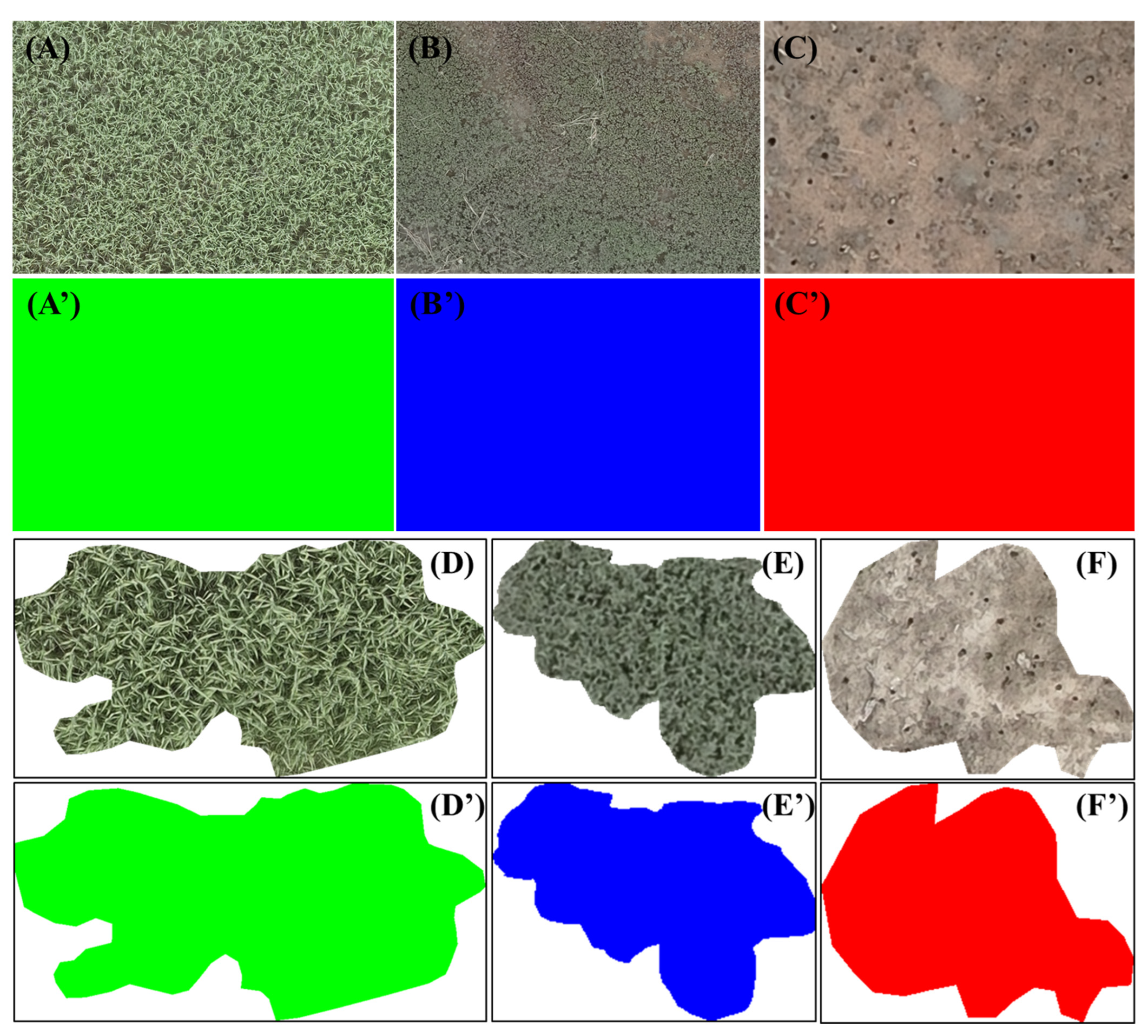
2.4. Vegetation Classification

The present study evaluated and compared the performance of two classification algorithms, namely maximum likelihood classification (MLC) and U-net, using very-high-resolution UAV-RGB imagery for the vegetation type and coverage mapping in Jujin Estuary. In our previous study, the MLC classifier showed the highest classification accuracy among the various supervised classification methods, such as Mahalanobis distance, minimum distance, and support vector machine. Therefore, in this study, only the MLC method was compared with U-net results for evaluating the classification performance.

2.4.1. Pixel-Based Classification

ENVI version 5.6 (L3HARRIS, Broomfield, CO, USA) software was used for pixel-based classification. The MLC algorithm maximizes the probability function that pixels of each class belong to a multivariate normal distribution and then divides it into the highest probabilistic class. Samples are divided into three categories as P. communis, S. maritima, and sediment. The training pixels for each of the desired classes were defined based on the identified area from the field survey using a region-of-interest (ROI) tool, and only 60% of them were used for training data. In order to select a good training area for a class, the uniformity and representativeness of each class throughout the whole image were considered. Here, the classification parameter was set as a default in the ENVI 5.6 software.

2.4.2. Deep-Learning Analysis

U-Net, as proposed previously [32], is an image-segmentation algorithm based on a convolution neural network. It is composed of a contracting path in the down-sampling process and an expansive path in the up-sampling process, with direct connections called skip-connections between the two paths; the skip-connections keep fine information from the original image, even in deep networks [33]. Figure 3 depicts the U-Net structure. In the contracting path, two convolution operations and one max-pooling operation are performed. This process is repeated three times, and deeper layers extract coarser features. In each iteration of the expansive path, one transpose convolution operation and two convolution operations are performed, and features from the contracting path are concatenated to maintain high-resolution features. Through the structure shown in the figure, all pixels of the input image can be classified into three classes.
Data labeling is an essential step in a supervised DL task. Various data-labeling methods may be used, such as bounding box, polygon, polyline, and point. In this research, the most commonly used methods, bounding box and polygon, were compared. The bounding box is the most commonly used method in image labeling, as it draws objects into rectangular boxes. However, in the case of a homogeneous area with a small size, large-sized image data cannot be created. Polygonal segmentation is another type of data annotation, in which complex polygons are used instead of rectangles to define the shape and location of the object more precisely; however, it requires more effort and time in image labeling. Figure 4 represents examples of training data generated using the two labeling methods. In each labeling method, all pixels of one selected area were set to the same classification, and the training dataset was constructed by extracting patches with specific sizes from the images. In the case of polygon annotation, the unclassified area was masked so that the loss was not computed during the learning stage.
In using images to train a model, there are physical limitations to using the whole area of a large image at once for learning. Accordingly, a large image may be divided into small patches and used for learning. For U-Net, the size of the patch used for training can affect model performance. Small training patches are advantageous for the model to learn detailed features; however, the training may not be able to sufficiently learn large features and may be biased. Large training patches are advantageous for learning common features of the training data, but detailed features may be ignored. In this study, we divided the training data of the polygon-annotation method into three patch sizes and compared the classification results. Learning was performed by extracting patches of 16, 32, and 64 pixels.

2.5. Classification Accuracy Assessment

Based on the field survey, regular validation points of 5-m intervals were generated in the high-resolution UAV-RGB image, and they were designated as P. communis, S. maritima, and sediment groups. A total of 428 points were sampled in the study area, and 276 points of P. communis, 50 points of S. maritima, and 102 points of sediment were designated (Figure 5). The accuracy assessment of five classification scenarios was conducted using the confusion matrix and kappa statistics. For overall accuracy, we divided the sum of the number of correctly identified pixels by the total number of reference data. In addition, errors of omission were calculated because it is possible that the overall accuracy might be quite high, whereas a considerable amount of errors can be included in individual classes or several classes. The kappa coefficient is an indicator of which percentage of the correct values of the confusion matrix are “true” agreement (value 1) versus “chance” agreement (value 0), computed based on the following formulation:
k = P 0 P e 1 P e ,  
where P0 is the observed agreement ratio and Pe is the hypothetical probability of chance agreement. The probabilities of each observer randomly seeing each category were calculated using the observed data. Pe is defined as follows:
P e = 1 N 2 k n k 1 n k 2 .
For k categories, N observations to categorize and nki the number of times rater i predicted category k. If the raters are in complete agreement then k = 1.

3. Results

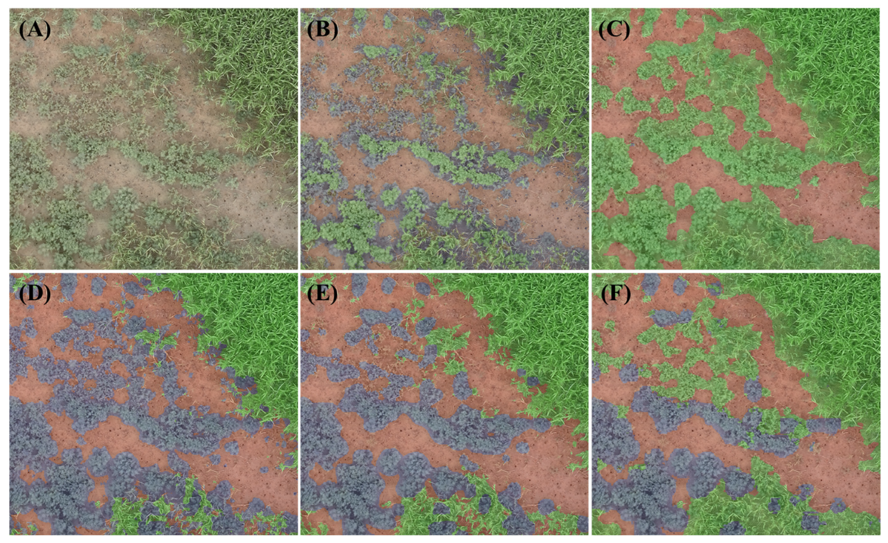
3.1. Classification of Salt Marsh Vegetation

In this study, we compared the classification performance of pixel-based and OBIA methods in salt marsh vegetation based on UAV-RGB data. This study focused on evaluating the classification accuracy of DL methods that have been widely used for the classification of mixed and dense vegetation. Among the various pixel-based classification methods, only the MLC method, which showed the highest accuracy in prior studies, was compared with the DL (U-Net) results. In addition, to provide proper comparative analyses, not only the labeling-annotation type (bounding box and polygon) but also different image-patch sizes (16 × 16, 32 × 32, and 64 × 64 pixels) were compared. However, in the case of bounding-box-based labeling, only the 64 × 64 pixel patch-size results, which were the most accurate in the prior study, were compared.
The MLC and U-Net classification results of five classification scenarios are presented in Figure 6. In all classification scenarios, based on tidal channel (TC) 1, the right side was mostly classified as P. communis, and the left side was classified as S. maritima. All classification maps were similar to the actual distribution of salt wetland vegetation species, which is generally consistent with the field survey data. However, unlike the U-Net classification results, many pixels were classified as S. maritima near TC 2 in the MLC result (Figure 6B versus Figure 6C–F). In addition, compared with other classification results, many pixels classified as S. maritima in the left part of TC 1 occupied a much larger area (Figure 6B).

3.2. Classification Performance

The accuracy assessment results of MLC and U-Net classifications are shown in Figure 7 and are listed in Table 1. As expected, MLC, a pixel-based classification method, showed the lowest OA at 73%, and some pixels were unclassified. Conversely, the U-Net classification method had an OA exceeding 90% in all classification scenarios; the highest OA of 93% was the result of U-Net classification of the 64 × 64 pixel patch size annotated with a polygon boundary. The kappa value was also the lowest in the MLC classification results; for all U-Net classification results, the kappa value exceeded 0.8. Overall, the combination of polygon annotation with the 64 × 64 sized patch extraction in the U-Net classifier showed the best classification performance, with a 93.0% OA and a kappa value of 0.863.
From the results of the field survey, greenish S. maritima was similar in color to P. communis, and reddish S. maritima was similar in color to sediment. In the vegetation classification results of the five scenarios (one MLC and four U-Net classification methods), the MLC method showed high omission errors in all of the P. communis, S. maritima, and sediment classes (Table 1). In particular, compared to the U-Net method, there were many pixels in which P. communis was misclassified as S. maritima. In the U-Net classification results, the omission error of P. communis was less than 10% in all scenarios, while the omission error tended to be high in the S. maritima class. Despite the higher than 90% OA in all U-Net-based scenarios, this approach showed more than 20% omission errors in one class (S. maritima or sediment), with the exception of the 16 × 16 pixel patch-size labeling method. Comparing the omission errors based on the annotation type in the U-Net classification method, the bounding-box method tended to misclassify sediment as S. maritima, while the polygon method tended to misclassify S. maritima as sediment.
In a comparison of the OA and kappa values, the best classification performance and lowest errors of omission were achieved with the U-Net classification method using polygon annotation and a 64 × 64 pixel patch size. To highlight the details of the classification results, Figure 8 and Figure 9 show magnifications of the same results (red and yellow rectangles in Figure 6). In this study, we tested whether it was possible to detect small patches of vegetation and to distinguish species in mixed vegetation. To this end, representative areas were selected in which small patches represented one species (yellow box in Figure 6A) and mixed vegetation included several species (red box in Figure 6A). In Figure 8 and Figure 9, the vegetation classification results overlapped with the original UAV-RGB image; P. communis is marked in green, S. maritima in blue, and sediment in red. Despite the sufficient OA in object segmentation of the U-Net classifier, it still showed poor classification performance on mixed and small patches of vegetation. In Figure 8A, P. communis and S. maritima were mixed. P. communis was mainly distributed in the upper right and lower center, and S. maritima was distributed in the rest of the area. In the MLC results, most S. maritima was misclassified as P. communis (Figure 8B). Despite the higher than 90% OA in the U-Net classification with bounding-box annotation, there was no distinction between P. communis and S. maritima in mixed vegetation (Figure 8C). In the U-Net classification results with polygon annotation, all three patch sizes were generally well distinguished between P. communis and S. maritima; however, some misclassified pixels were found in the 64 × 64 pixel patch-size labeling, in which S. maritima was misclassified as P. communis (Figure 8D–F).
Figure 9 shows a detailed comparison of the results of vegetation classification on small patches using the MLC and U-Net methods. Although only S. maritima species inhabits this area, some pixels were misclassified as P. communis in the MLC results (Figure 9B). In the U-Net classification results labeled with a 64 × 64 pixel patch size, S. maritima was not detected in the yellow circle (Figure 9C,F). Moreover, the U-Net classification with bounding-box annotation showed an overestimated result compared to the actual vegetation patch size (Figure 9C). Overall, small polygon-type patches of 16 × 16 and 32 × 32 pixels in size in the U-Net classifier provided the best accuracy (Figure 9D,E).

4. Discussion

In remote sensing, flight altitude significantly impacts the spatial resolution that determines whether species can be identified in a vegetation community [25,30]. In the case of satellite imagery, it is difficult to obtain images of sufficient spatial resolution for vegetation classification at the species level due to the limited ground sampling distance at altitudes exceeding hundreds of kilometers. Aerial photographs collected at lower altitudes ensure sufficient spatial resolution to distinguish halophyte species but are not suitable for repeated surveys due to limited operating costs and time. Conversely, UAV data can be used to identify halophyte communities at a low cost with ultra-high spatial resolution; it also has the advantages of non-destructive surveying, flexible mapping schedule, rapid response to habitat change, and ease of multi-temporal monitoring. Combined with RGB sensors, high classification accuracy of vegetation can be achieved, despite lacking the spectral information of multi-band sensors.
The species distribution of salt marsh vegetation can be characterized in terms of the combined influences of topography, saline adaptation, and flooding regimes [34,35]; therefore, at the landscape level, it is an important factor for estimating vegetation distribution. However, if there are many small patch areas or if there is a mixture of several vegetation species, as in this study, a better classification method is needed. Moreover, if the same vegetation species are displayed in various colors, it is more difficult to classify them with high accuracy using existing pixel-based classification algorithms. This study demonstrated the advantages of combining UAV-RGB data and DL using a U-Net classifier for vegetation classification of salt marshes. In particular, species classification is possible with high accuracy in small patches and mixed vegetation in this type of study area. Previous studies have attempted to classify vegetation using multi-spectral, hyperspectral, and lidar sensor data; however, the spectral information of RGB sensors is limited [18,30,31]. An attempt at vegetation classification by combining RGB and lidar data showed that the correlation between lidar measurements and field values improved from R2 values of 0.79 to 0.94 [36]. Meanwhile, a proposed hyperspectral band-based vegetation index, namely the hyperspectral image-based vegetation index, had a vegetation extraction accuracy exceeding 90% [37]. In this regard, the classification accuracy of more than 90% of the current study is even more significant, in that our method can easily be applied to other vegetation mappings and classifications in terms of UAVs coupled with RGB sensors.
Typically, remote-sensing classification of salt marshes is performed using pixel-based analysis and OBIA classification. In this study, as an OBIA method, the classification performance of DL-based U-Net classifiers was compared with a pixel-based classification method. As expected, the U-Net classification results showed a significant improvement in accuracy compared to the pixel-based results (Table 1). Pixel-based classification uses only spectral information. However, the U-Net classifier uses similar features that are segmented into meaningful pixel groups and then automatically learns features (spectral, spatial, contextual, and textual information) through training. Then, the ML algorithm is used to produce the final classification result. Several studies have demonstrated the higher classification accuracy of OBIA methods in the remote-sensing monitoring of coastal wetlands [20,25]. These results are consistent with a previous study [21] showing that the three DL methods (U-Net, DeepLabV3+, and PSPNet) had the best performance in classifying wetland vegetation compared with the pixel-based classification result.
Unexpectedly, the OA of the U-Net classifications exceeded 90%, regardless of the annotation type (bounding box versus polygon). In general, for objects that are not rectangular, a bounding box is not sufficiently precise. However, there was no significant difference in accuracy between the two annotation types in this study. There are two possible assumptions in this regard. First, P. communis pixels showed very high classification accuracy in both methods, such that even if some pixels of S. maritima and sediment were misclassified, they did not significantly affect the OA. Second, the verification points were set at intervals of 5 m; this verification point was not located at the boundary between targets that generated many classification errors. There was no significant difference in OA between the bounding box and polygon methods, but there was a significant difference in the classification performances for small patches and mixed vegetation (Figure 8 and Figure 9). Similar to the results of previous studies, better classification performance can be obtained through the application of polygon, rather than bounding-box, annotation. In addition, although the difference in OA according to the data-labeling size was not significant, the results confirmed that smaller labeling sizes were even more effective for classifying small patches and mixed vegetation. Polygon annotation is much more refined but requires more time and effort than box annotation. Therefore, we recommend the bounding-box method for studies of simple vegetation distributions and large research areas, as it is much quicker and provides sufficient accuracy under these circumstances.
In more recent studies, coastal wetland vegetation (e.g., mangroves, salt marshes, and seagrasses) has attracted attention as “blue carbon” because coastal wetlands sequester carbon more effectively than terrestrial forests [38,39,40,41]. Therefore, many researchers are conducting vegetation mapping studies using remote-sensing data, in an attempt to estimate the carbon flux [42]. However, the outcomes vary widely with vegetation type, and many have run into problems in accurately distinguishing various species [43,44]. Moreover, most studies have had difficulty detecting small patches and accurately identifying the species in mixed vegetation using satellite imagery with relatively low spatial resolutions [22,45,46]. In the results of the current study, accurate classification of salt marsh vegetation species was possible by combining a DL U-Net classifier with high-resolution UAV-RGB images. We expect our approach to help yield more accurate blue-carbon estimations in future studies.

5. Conclusions

This study aimed at providing mappings of salt marsh vegetation using image segmentation. For this, we applied pixel-based (MLC) and DL (U-Net) classifiers to high-resolution UAV images. The MLC method showed an OA of 73%, whereas the U-Net technique OA ranged from 90.0% to 93.0%.
The highest OA results were derived when applying polygon annotation with a labeling size of 64 × 64 pixels in U-Net classification (OA = 93.0%, kappa value = 0.863). However, the use of labeling data with 16 × 16 and 32 × 32 pixel patch sizes led to better discrimination in detecting small patches and classifying species in mixed vegetation. In conclusion, this study confirms the utility of the U-Net classifier in classifying salt marsh vegetation. However, since the polygon-annotation method and small labeling patch size increase the dataset, calculation time, and hardware requirements, it is necessary to choose a method that well reflects the characteristics of the study area (study-site scale, amount of data, vegetation distribution pattern, etc.). Taking advantage of computational efficiency, the application of the U-Net model is expected to be practical and sustainable for regional long-term monitoring.
Mapping coastal marshes is a challenging task because of their natural characteristics, such as heterogeneous distributions and seasonality. Notably, salt marsh vegetation undergoes seasonal color change; thus, vegetation classification considering seasonal change is necessary for our ongoing work. In future studies, additional labeling data will be established considering seasonal changes in salt marsh vegetation. It would be expected that we could develop an advanced model that extracts the common features of the objective target with the data. Additionally, we are in the process of developing an algorithm that can estimate not only the distribution of vegetation but also the biomass, through canopy-height estimation based on UAV images. These additional studies are expected to contribute substantially to efforts in accurately estimating the blue carbon of salt marshes, as opposed to methods that use only vegetation-distribution areas. Furthermore, accurate salt marsh mapping can provide basic information for environmental management, restoration, and conservation planning for these vital wetland ecosystems.

Author Contributions

Conceptualization, K.K. and J.-H.R.; methodology, D.L., C.-H.K. and H.-T.J.; software, Y.J.; validation, K.K., J.-H.R. and H.-T.J.; formal analysis, Y.J. and J.L.; investigation, K.K., Y.J. and J.L.; data curation, K.K. and Y.J.; writing—original draft preparation, K.K.; writing—review and editing, K.K. and J.-H.R.; visualization, K.K. and Y.J.; supervision, J.-H.R.; funding acquisition, J.-H.R. All authors have read and agreed to the published version of the manuscript.

Funding

This research was supported by the project “Development of technology for constructing biological and environmental spatial information system of tidal flats through machine learning of remotely sensed visual data (PEA0115)” funded by the Korea Institute of Ocean Science and Technology.

Data Availability Statement

Not applicable.

Acknowledgments

The authors would like to thank Han Jun Woo (Korea Institute of Ocean Science and Technology) and Byeong-Mee Min (Dankook University) for their advice.

Conflicts of Interest

The authors declare no conflict of interest.

References

  1. Barbier, E.B.; Hacker, S.D.; Kennedy, C.; Koch, E.W.; Stier, A.; Silliman, B. The value of estuarine and coastal ecosystem services. Ecol. Monogr. 2011, 81, 169–193. [Google Scholar] [CrossRef]
  2. Lau, W. Beyond carbon: Conceptualizing payments for ecosystem services in blue forests on carbon and other marine and coastal ecosystem services. Ocean Coast. Manag. 2013, 83, 5–14. [Google Scholar] [CrossRef]
  3. Gailis, M.; Kohfeld, K.E.; Pellatt, M.G.; Garlson, D. Quantifying blue carbon for the largest salt marsh in southern British Columbia: Implications for regional coastal management. Coast. Eng. J. 2021, 3, 275–309. [Google Scholar] [CrossRef]
  4. Zhu, Q.; Wiberg, P.L. The Importance of Storm Surge for Sediment Delivery to Microtidal Marshes. JGR Earth Surf. 2022, 127, e2022JF006612. [Google Scholar] [CrossRef]
  5. Gedan, K.B.; Siliman, B.R.; Bertness, M.D. Centuries of human-driven change in salt marsh ecosystems. Annu. Rev. Mar. Sci. 2009, 1, 117–141. [Google Scholar] [CrossRef]
  6. Perrino, E.V.; Wagensommer, R.P. Crop Wild Relatives (CWRs) Threatened and Endemic to Italy: Urgent Actions for Protection and Use. Biology 2022, 11, 193. [Google Scholar] [CrossRef]
  7. Tomaselli, V.; Mantino, F.; Tarantino, C.; Albanese, G.; Adamo, M. Changing landscapes: Habitat monitoring and land transformation in a long-time used Mediterranean coastal wetland. Wetl. Ecol. Manag. 2023, 31, 31–58. [Google Scholar] [CrossRef]
  8. Shuman, C.S.; Ambrose, R.F. A Comparison of Remote Sensing and Ground-Based Methods for Monitoring Wetland Restoration Success. Restor. Ecol. 2003, 11, 325–333. [Google Scholar] [CrossRef]
  9. Zedler, J.B.; Kercher, S. Wetland Resources: Status, Trends, Ecosystem Services, and Restorability. Annu. Rev. Environ. Resour. 2005, 30, 39–74. [Google Scholar] [CrossRef]
  10. Guo, M.; Li, J.; Sheng, C.; Xu, J.; Wu, L. A review of Wetland Remote Sensing. Sensors 2017, 17, 777. [Google Scholar] [CrossRef]
  11. Sun, C.; Fagherazzi, S.; Liu, Y. Classification mapping of salt marsh vegetation by flexible monthly NDVI time-series using Landsat imagery. Estuar. Coast. Shelf Sci. 2018, 213, 61–80. [Google Scholar] [CrossRef]
  12. Meneses, N.C.; Brunner, F.; Baier, S.; Geist, J.; Schneider, T. Quantification of Extent, Density, and Status of Aquatic Reed Beds Using Point Clouds Derived from UAV–RGB Imagery. Remote Sens. 2018, 10, 1869. [Google Scholar] [CrossRef]
  13. Samiappan, S.; Turnage, G.; Hathcock, L.A.; Moorhead, R. Mapping of invasive phragmites (common reed) in Gulf of Mexico coastal wetlands using multispectral imagery and small unmanned aerial systems. Int. J. Remote Sens. 2017, 38, 2861–2882. [Google Scholar] [CrossRef]
  14. Doughty, C.L.; Ambrose, R.F.; Okin, G.S.; Cavanaugh, K.C. Characterizing spatial variability in coastal wetland biomass across multiple scales using UAV and satellite imagery. Remote Sens. Ecol. Conserv. 2021, 7, 411–429. [Google Scholar] [CrossRef]
  15. Martin, R.; Brabyn, L.; Beard, C. Effects of class granularity and cofactors on the performance of unsupervised classification of wetlands using multi-spectral aerial photography. J. Spat. Sci. 2014, 59, 269–282. [Google Scholar] [CrossRef]
  16. Everitt, J.H.; Yang, C.; Davis, M.R.; Everitt, J.H.; Davis, M.R. Mapping wild taro with color-infrared aerial photography and image processing. J. Aquat. Plant. Manag. 2007, 45, 106–110. [Google Scholar]
  17. Pande-Chhetri, R.; Abd-Elrahman, A.; Liu, T.; Morton, J.; Wilhelm, V.L. Object-Based Classification of Wetland Vegetation Using Very High-Resolution Unmanned Air System Imagery. Eur. J. Remote Sens. 2017, 50, 564–576. [Google Scholar] [CrossRef]
  18. Sibaruddin, H.I.; Shafri, H.Z.M.; Pradhan, B.; Haron, N.A. Comparison of pixel-based and object-based image classification techniques in extracting information from UAV imagery data. IOP Conf. Ser. Earth Environ. Sci. 2018, 169, 012098. [Google Scholar] [CrossRef]
  19. Dronova, I. Object-Based Image Analysis in Wetland Research: A Review. Remote Sens. 2015, 7, 6380–6413. [Google Scholar] [CrossRef]
  20. Durgan, S.D.; Zhang, C.; Duecaster, A.; Fourney, F.; Su, H. Unmanned Aircraft System Photogrammetry for Mapping Diverse Vegetation Species in a Heterogeneous Coastal Wetland. Wetlands 2020, 40, 2621–2633. [Google Scholar] [CrossRef]
  21. Zheng, J.-Y.; Hao, Y.-Y.; Wang, Y.-C.; Zhou, S.-Q.; Wu, W.-B.; Yuan, Q.; Gao, Y.; Guo, H.-Q.; Cai, X.-X.; Zhao, B. Coastal Wetland Vegetation Classification Using Pixel-Based, Object-Based and Deep Learning Methods Based on RGB-UAV. Land 2022, 11, 2039. [Google Scholar] [CrossRef]
  22. Adam, E.; Mutanga, O.; Rugrgr, D. Multispectral and hyperspectral remote sensing for identification and mapping of wetland vegetation: A review. Wetl. Ecol. Manag. 2010, 18, 281–296. [Google Scholar] [CrossRef]
  23. Kamal, M.; Phinn, S. Hyperspectral data for mangrove species mapping: A comparison of pixel-based and object-based approach. Remote Sens. 2011, 3, 2222–2242. [Google Scholar] [CrossRef]
  24. Gao, Y.; Li, W.; Zhang, M.; Wang, J.; Sun, W.; Tao, R.; Du, Q. Hyperspectral and Multispectral Classification for Coastal Wetland Using Depthwise Feature Interaction Network. IEEE Trans. Geosci. Remote Sens. 2022, 60, 5512615. [Google Scholar] [CrossRef]
  25. Owers, C.J.; Rogers, K.; Woodroffe, C.D. Identifying Spatial Variability and Complexity in Wetland Vegetation Using an Object-Based Approach. Int. J. Remote Sens. 2016, 37, 4296–4316. [Google Scholar] [CrossRef]
  26. Correll, M.D.; Hantson, W.; Hodgman, T.P.; Cline, B.B.; Elphick, C.S.; Gregory Shriver, W.; Tymkiw, E.L.; Olsen, B.J. Fine-Scale Mapping of Coastal Plant Communities in the Northeastern USA. Wetlands 2019, 39, 17–28. [Google Scholar] [CrossRef]
  27. Bhatnagar, S.; Gill, L.; Ghosh, B. Drone Image Segmentation Using Machine and Deep Learning for Mapping Raised Bog Vegetation Communities. Remote Sens. 2020, 12, 2602. [Google Scholar] [CrossRef]
  28. Lee, J.S.; Kim, J.W. Dynamics of zonal halophyte communities in salt marshes in the world. J. Mar. Isl. Cult. 2018, 7, 84–106. [Google Scholar] [CrossRef]
  29. Park, J.W. Studies on the Characteristics of Distribution and Environmental Factor of Halophyte Vegetation in Western and Southern Coast in Korea. Master’s Thesis, Graduate School of Kongju National University, Gongju, Republic of Korea, 2021; p. 123, (Korean with English Abstract). [Google Scholar]
  30. Park, S.I.; Hwang, Y.S.; Um, J.S. Estimating blue carbon accumulated in a halophyte community using UAV imagery: A case study of the southern coastal wetlands in South Korea. J. Coast. Res. 2021, 25, 38. [Google Scholar] [CrossRef]
  31. Chung, S.H. Features and Functions of Purple Pigment Compound in Halophytic Plant Suaeda japonica: Antioxidant/Anticancer Activities and Osmolyte Function in Halotolerance. Korean J. Plant Res. 2021, 31, 342–354. [Google Scholar]
  32. Ronneberger, O.; Fischer, P.; Brox, T. U-Net: Convolutional Networks for Biomedical Image Segmentation. In Proceedings of the Medical Image Computing and Computer-Assisted Intervention—MICCAI 2015: 18th International Conference, Munich, Germany, 5–9 October 2015; Springer: Cham, Switzerland, 2015; pp. 234–241. [Google Scholar]
  33. Mandelli, S.; Lipari, V.; Bestagini, P.; Tubaro, S. Interpolation and Denoising of Seismic Data using Convolutional Neural Networks. arXiv 2019, arXiv:1901.07927. [Google Scholar]
  34. Isacch, J.P.; Costa, C.S.B.; Rodríguez-Gallego, L.; Conde, D.; Escapa, M.; Gagliardini, D.A.; Iribarne, O.O. Distribution of saltmarsh plant communities associated with environmental factors along a latitudinal gradient on the south-west Atlantic coast. J. Biogeogr. 2006, 33, 888–900. [Google Scholar] [CrossRef]
  35. Li, S.; Ge, Z.; Xie, L.; Chen, W.; Yuan, L.; Wang, D.; Li, X.; Zhang, L. Ecophysiological response of native and exotic salt marsh vegetation to waterlogging and salinity: Implications for the effects of sea level rise. Sci. Rep. 2018, 8, 2441. [Google Scholar] [CrossRef]
  36. Curcio, A.C.; Peralta, G.; Aranda, M.; Barbero, L. Evaluating the Performance of High Spatial Resolution UAV-Photogrammetry and UAV-LiDAR for Salt Marshes: The Cádiz Bay Study Case. Remote Sens. 2022, 14, 3582. [Google Scholar] [CrossRef]
  37. Sun, G.; Jiao, Z.; Zhang, A.; Li, F.; Fu, H.; Li, Z. Hyperspectral image-based vegetation index (HSVI): A new vegetation index for urban ecological research. Int. J. Appl. Earth Observ. Geoinform. 2021, 103, 102529. [Google Scholar] [CrossRef]
  38. Alongi, D.M. Carbon Sequestration in Mangrove Forests. Carb. Manag. 2012, 3, 313–322. [Google Scholar] [CrossRef]
  39. Chmura, G.L.; Anisfeld, S.C.; Cahoon, D.R.; Lynch, J.C. Global carbon sequestration in tidal, saline wetland soils. Glob. Biogechem. Cycles 2003, 17, 1111. [Google Scholar] [CrossRef]
  40. Macreadie, P.I.; Costa, M.D.; Atwood, T.B.; Friess, D.A.; Kelleway, J.J.; Kennedy, H.; Lovelock, C.E.; Serrano, O.; Durte, C.M. Blue Carbon as a Natural Climate Solution. Nat. Rev. Earth Environ. 2021, 2, 826–839. [Google Scholar] [CrossRef]
  41. Wang, F.; Sanders, C.J.; Santos, I.R.; Tang, J.; Schuerch, M.; Kirwan, M.L.; Kopp, R.E.; Zhu, K.; Li, X.; Yuan, J.; et al. Global blue carbon accumulation in tidal wetlands increases with climate change. Natl. Sci. Rev. 2021, 8, nwaa296. [Google Scholar] [CrossRef]
  42. Pham, T.D.; Xia, J.; Ha, N.T.; Bui, D.T.; Le, N.N.; Takeuchi, W. A Review of Remote Sensing Approaches for Monitoring Blue Carbon Ecosystems: Mangroves, Seagrasses and Salt Marshes during 2010–2018. Sensors 2019, 19, 1933. [Google Scholar] [CrossRef]
  43. Kauffman, J.B.; Heider, C.; Cole, T.G.; Dwire, K.A.; Donato, D.C. Ecosystem carbon stocks of Micronesian mangrove forests. Wetlands 2011, 31, 343–352. [Google Scholar] [CrossRef]
  44. Radabaugh, K.R.; Moyer, R.P.; Chappel, A.R.; Powell, C.E.; Bociu, I.; Clark, B.C.; Smoak, J.M. Coastal Blue Carbon Assessment of Mangroves, Salt Marshes, and Salt Barrens in Tampa Bay, Florida, USA. Estuaries Coasts 2018, 41, 1496–1510. [Google Scholar] [CrossRef]
  45. Meng, X.; Shang, N.; Zhang, X.; Li, C.; Zhao, K.; Qiu, X.; Weeks, E. Photogrammetric UAV Mapping of Terrain under Dense Coastal Vegetation: An Object-Oriented Classification Ensemble Algorithm for Classification and Terrain Correction. Remote Sens. 2017, 9, 1187. [Google Scholar] [CrossRef]
  46. Wang, C.; Menenti, M.; Stoll, M.-P.; Belluco, E.; Marani, M. Mapping mixed vegetation communities in salt marshes using airborne spectral data. Remote Sens. Environ. 2007, 107, 559–570. [Google Scholar] [CrossRef]
Figure 1. Study area in Jujin Estuary on the western coast of Korea. A magnified portion of the red rectangle is displayed in Figure 2.
Remotesensing 15 02723 g001
Figure 2. Orthophoto mosaic image of the study area from UAV data collected on 25 June 2021. (A) The distribution of two salt marsh vegetation samples and sediment samples in Jujin Estuary (Google Maps). Enlarged unmanned aerial vehicle images of representative vegetation of (B) greenish Suaeda maritima, (C) reddish S. maritima, and (D) Phragmites communis.
Remotesensing 15 02723 g002
Figure 3. The U-Net model architecture used in this study with an input sample size of 32 × 32 pixels as an example.
Remotesensing 15 02723 g003
Figure 4. Example of labeled images. The labeled and training samples were created using the (AC) bounding-box and (DF) polygon-annotation methods applied to unmanned aerial vehicle-red–green–blue images. The representative labeling data of (AD) Phragmites communis, (B,E) Suaeda maritima, and (CE) sediment. (A’F’) Sample images from labeling dataset and their annotations (P. communis is marked in green, S. maritima in blue, and sediment in red).
Remotesensing 15 02723 g004
Figure 5. Locations of 276 verification points in the study area as shown by an unmanned aerial vehicle-red–green–blue image. The reference data were selected at intervals of 5 m, and Phragmites communis, Suaeda maritima, and sediment are marked in red, magenta, and yellow, respectively.
Remotesensing 15 02723 g005
Figure 6. Classification results of five classification scenarios: (A) original image, (B) maximum likelihood, (C) U-Net with bounding box and 64 × 64 pixel patch-size annotation, (D) U-Net with polygon and 16 × 16 pixel patch-size annotation, (E) U-Net with polygon and 32 × 32 pixel patch-size annotation, and (F) U-Net with polygon and 64 × 64 pixel patch-size annotation. TC: tidal channel.
Remotesensing 15 02723 g006
Figure 7. Errors of omission (%) and overall accuracy (%) for maximum likelihood classification (MLC) and U-Net classification with different data-annotation types and sizes of extraction patches.
Remotesensing 15 02723 g007
Figure 8. Representative area for the comparison of classification performance in mixed vegetation (red box in Figure 6A): (A) original image, (B) maximum likelihood, (C) U-Net with bounding box and 64 × 64 patch-size annotation, (D) U-Net with polygon and 16 × 16 pixel patch-size annotation, (E) U-Net with polygon and 32 × 32 pixel patch-size annotation, and (F) U-Net with polygon and 64 × 64 patch-size annotation.
Remotesensing 15 02723 g008
Figure 9. Representative area for a comparison of the classification performance in small patches with one species (yellow box in Figure 6A): (A) original image, (B) maximum likelihood, (C) U-Net with bounding box and 64 × 64 pixel patch-size annotation, (D) U-Net with polygon and 16 × 16 pixel patch-size annotation, (E) U-Net with polygon and 32 × 32 pixel patch-size annotation, and (F) U-Net with polygon and 64 × 64 pixel patch-size annotation.
Remotesensing 15 02723 g009
Table 1. Accuracy assessment results for maximum likelihood classification (MLC) and U-Net classifications. OA; overall accuracy, PA; producer’s accuracy, and UA; user’s accuracy.
MethodReference Data
MLC P. communisS. maritimaSedimentTotalKappa (SE)
P. communis203112050.562
(±0.032)
S. maritima673829134
Sediment397183
unclassified3216
Total27650102428
OA (%)72.9
PA (%)73.676.069.6
UA (%)99.028.485.5
U-Net (64 × 64)
Bounding box
P. communisS. maritimaSedimentTotalKappa (SE)
P. communis269242750.843
(±0.024)
S. maritima4451967
Sediment337985
Total27650102
OA (%)91.8
PA (%)97.590.077.5
UA (%)97.866.292.9
U-Net (16 × 16)
Polygon
P. communisS. maritimaSedimentTotalKappa (SE)
P. communis249002490.815
(±0.026)
S. maritima1842868
Sediment9894111
Total27650102
OA (%)90.0
PA (%)90.284.092.2
UA (%)100.061.884.7
U-Net (32 × 32)
Polygon
P. communisS. maritimaSedimentTotalKappa (SE)
P. communis259012600.817
(±0.026)
S. maritima1038553
Sediment71296115
Total27650102
OA (%)91.8
PA (%)93.876.094.1
UA (%)99.671.783.5
U-Net (64 × 64)
Polygon
P. communisS. maritimaSedimentTotalKappa (SE)
P. communis270332760.863
(±0.023)
S. maritima233439
Sediment41495113
Total27650102
OA (%)93.0
PA (%)97.866.093.1
UA (%)97.884.684.1
Disclaimer/Publisher’s Note: The statements, opinions and data contained in all publications are solely those of the individual author(s) and contributor(s) and not of MDPI and/or the editor(s). MDPI and/or the editor(s) disclaim responsibility for any injury to people or property resulting from any ideas, methods, instructions or products referred to in the content.

