Monitoring the Impact of Heat Damage on Summer Maize on the Huanghuaihai Plain, China

Abstract

As an important food crop, summer maize is widely planted all over the world. Monitoring its growth and output is of great significance for world food security. With the trend of global warming and deterioration, the frequency of high temperature and heat damage affecting summer corn has been increasing in the past ten years. Therefore, there is an increasing demand for monitoring the high temperature and heat damage of summer maize. At present, there are nearly a hundred indices or methods for research on high temperature and heat damage. However, research based on the vegetation index cannot fully describe the damage caused by high-temperature thermal damage, and there is an obvious asynchrony effect. Research based on hyperspectral remote sensing has many inconveniences in data acquisition and complex physical model construction. Therefore, this study uses remote sensing data, including MODIS surface reflection data, MODIS land surface temperature products, as well as ground observation data and statistical data, combined with multiple remote sensing indices and land surface temperature, to construct a remote sensing index, LSHDI (land surface heat damage index). The LSHDI first searches for a location with the worst vegetation growth conditions in the three-dimensional feature space based on the LST (land surface temperature), the normalized difference vegetation index (NDVI), and the land surface water index (LSWI). Then, it calculates the distance between each point and this location to measure the degree of vegetation affected by high temperature and heat damage. Finally, because there is no reliable disaster verification dataset that has been published at present, this study uses soil moisture as a reference to explain the performance and stability of the LSHDI. The results showed that their coefficient of determination was above 0.5 and reached a significance level of 0.01. The LSHDI can well-reflect the high temperature and heat damage of land surface vegetation and can provide important data support and references for agricultural management departments.

1. Introduction

High-temperature heat damage is an extreme climatic phenomenon caused by excessively high temperatures. It causes extensive damage to ecosystems and seriously affects the occurrence of the social economy. In agricultural production, high-temperature heat damage is specifically manifested as damage to crop growth and yield caused by high temperatures, which is generally caused by the temperature exceeding the upper limit temperature of crop growth. There are many methods for the study of high-temperature heat damage, such as the commonly used agrometeorological indicators [1,2,3,4]. According to the critical threshold of the daily average temperature and the daily maximum temperature, and the number of continuous days, the high-temperature and thermal damage levels of crops can be judged. There are also a variety of remote sensing indices that reflect the growth status of vegetation, which are used to indirectly infer the levels of high temperature and heat damage on crops. To accurately describe and predict heat damage, nearly one hundred monitoring and early-warning methods for high-temperature thermal damage have been developed at home and abroad [5].

The traditional high-temperature heat damage index is constructed by expressing one or more variables (such as temperature and precipitation) as a single value to quantitatively characterize the degree of heat damage. Compared with the original variables, the high-temperature heat damage index obtained by this calculation contains more information and is more suitable for regional-scale, thermal-damage monitoring. According to the method of data acquisition, the traditional high-temperature heat damage index can be divided into three groups, based on the statistical data of the meteorological observatory, the remote sensing observation data, or a combination of the two. These include the Palmer drought severity index (PDSI) and the standardized precipitation evapotranspiration index (SPEI) based on station observation data of temperature and precipitation [6,7]. Among them, the PDSI also combines soil moisture and other physical observations and judges the surface drought by analyzing the soil moisture balance. It is of great significance in the statistics of affected areas, analysis of the temporal and spatial characteristics of drought, and drought prediction [8,9]. The high-temperature heat damage index established based on remote sensing data can be used to monitor the land surface conditions in a longer time series and on a larger spatial scale. The temperature condition index (TCI) normalizes the land surface temperature (LST), and it can be used to study the response of vegetation growth to temperature changes [10]. The precipitation condition index (PCI) and soil moisture condition index (SMCI) normalize precipitation and soil moisture content, respectively, and both represent the moisture condition of the physiological environment where the vegetation is located, which can infer the high temperature of the vegetation [9,10]. In addition, the PDI (perpendicular drought index), LSWI (land surface water index), NDWI (normalized difference water index), VSWI (vegetation supply water index), and the GVMI (global vegetation moisture index) have been widely used in monitoring research on land surface heat damage or drought [11,12]. In contrast, monitoring of high temperature and heat damage based on remote sensing data can largely compensate for the uneven distribution of ground stations and the lack of data; that is, in areas where the stations are sparsely distributed, remote sensing data can have a greater advantage.

Remote sensing data can monitor the physiological conditions of vegetation on a large spatial scale, and the growth of vegetation can be indirectly reflected through remote sensing images. For example, the normalized difference vegetation index (NDVI) and enhanced vegetation index (EVI) calculated from remote sensing reflectance data can quantify the greenness or coverage of land surface vegetation, and some studies can indirectly infer the changes in the vegetation growth environment by analyzing the changing spatiotemporal characteristics of these vegetation indices. In drought-affected areas, the NDVI value is generally low. The NDVI value and the growth status of the vegetation show a positive correlation trend [13]. Ji et al. studied the relationship between the NDVI and various drought indices and found that the NDVI has a strong correlation with land surface drought; therefore, it can be used as an indicator for monitoring drought events [14]. Boschetti et al. studied and analyzed the relationship between the NDVI and precipitation and proved that NDVI values can reflect the intensity of vegetation photosynthesis [15]. Compared with the NDVI, the EVI contains observation information in the blue band, which can reduce the influence of the atmosphere and soil background to a certain extent [16]. Additionally, in drought-affected areas, the changes in the EVI are consistent with changes in vegetation optical thickness and total land water storage. In addition, the vegetation condition index (VCI) normalizes the NDVI, which highlights the relative change in vegetation coverage in the study area [17]. The various abovementioned vegetation indices can reflect the degree and scope of thermal damage in a certain period of time in the study area, but there are temporal and spatial variations in the time of high-temperature heat damage events. In view of this, these indices will have different grading standards when used in different regions, resulting in poor comparability of the monitoring results between different pixels. To solve the deficiencies of the above indices, some studies have combined land surface temperature and vegetation indices to construct a variety of monitoring indices that can characterize the relative drought of an area, such as the TVDI (temperature vegetation dryness index) and VTCI (vegetation temperature condition index). The TVDI combines the NDVI and LST, and it analyzes the two-dimensional feature space constructed by the two, which can effectively characterize soil moisture information, thereby inferring the relative drought degree of a certain area [18]. The VTCI is similar to the TVDI, and it determines the dry edge and wet edge in the specific two-dimensional space of NDVI–LST. It not only considers the change in the NDVI in the area but also considers the change in LST under the same NDVI value. Both have the characteristics of local specificity and time domain specificity [19,20,21]. However, the above two indices have higher requirements for the selection of the study area, and the monitoring results are also affected by the vegetation coverage.

Although traditional remote sensing indices can characterize the physiological state of vegetation, the chlorophyll content in plants responds slowly to temperature or moisture. Therefore, remote sensing images cannot reflect the environment of the vegetation at that time in real time. There is a certain lag in remote sensing data. In addition, the vegetation index cannot capture early photosynthesis changes, which also limits the application of this type of remote sensing index in high-temperature and heat damage monitoring [22]. Since hyperspectral remote sensing data are mostly obtained through manual real-time field measurement, the data band information is more abundant, which not only guarantees the timeliness of the data but also obtains the information that cannot be detected in the wide-band remote sensing image. At present, there have been many studies using hyperspectral remote sensing to retrieve crop-leaf, plant, and canopy water content [23,24,25]. These research methods are generally divided into three groups: statistical methods, physical model methods, and spectral reflectance methods [26,27]. Crops have different irrigation amounts in different growth periods, and precise inversion of canopy water content is an important means to monitor the high temperature and heat damage of crops. The canopy absorption of the photosynthetically active radiation ratio, FAPAR (fraction of absorbed photosynthetically active radiation), can be used to describe the process of vegetation material and energy exchange and can indirectly reflect the status of vegetation or crops subjected to water and temperature stress [28,29,30]. There have been many published FAPAR inversion studies based on hyperspectral remote sensing [31,32,33], but thus far, comparative studies between various FAPAR inversion models are still lacking, and each model has different applicable scenarios. Therefore, to accurately monitor and analyze the high temperature and thermal damage of crops, choosing a suitable FAPAR inversion model and improving the accuracy of the existing inversion model are still important research directions in this field.

There are similarities and differences between high temperatures and drought, and many monitoring indicators and methods between the two can be shared. When high-temperature heat damage reaches a certain stage and causes a lack of vegetation or land surface water, it evolves into drought. High-temperature heat damage emphasizes the influence of temperature on vegetation, while drought focuses on land surface water [34,35,36]. In addition, research on high-temperature heat damage focuses on vegetation or crops, while the object of drought is not limited to vegetation; instead, it characterizes the impact of water loss on the entire land surface area, and the research focuses on land conditions [37,38,39,40]. When there is not much vegetation coverage in the study area, the study of surface drought is still of great significance. In contrast, it is meaningless to study the high temperature and heat damage of the surface without vegetation cover. This study focuses on the growth and development of vegetation and on the impact of temperature on crops; therefore, high-temperature heat damage is the research theme.

High-temperature heat damage research based on the traditional high-temperature heat damage index uses a general data spatial resolution, and the monitoring accuracy can still be improved. Research based on the vegetation index cannot fully describe the damage caused by high temperatures, and there is a relatively obvious lag. Research based on hyperspectral remote sensing has many inconveniences in data acquisition and complex physical model construction [41,42,43,44,45]. Therefore, this study uses remote sensing data with high temporal resolutions, including MODIS surface reflection data and MODIS land surface temperature products to extract vegetation temperature-sensitive bands, and combines LST to construct a remote sensing index, LSHDI (land surface heat damage index), which can more comprehensively reflect the growth environment of vegetation. This study also analyzes the trend in the LSHDI to obtain the temporal and spatial changes in the study area.

2. Materials and Methods

2.1. Study Area

The Huanghuaihai Plain is the main production area of summer maize in China, and includes three regions: North China, East China, and Central China (32°~40°N, 105°~121°E). The annual precipitation in this area is 500–900 mm, of which July–August precipitation accounts for approximately 45–65% of the annual precipitation [46]. The average elevation of the Huanghuaihai Plain is below 50 m. Its climatic conditions and flat terrain advantages in the same period of rain and heat make it an important farming area, and its arable land accounts for approximately 25% of the country’s total arable land. The main forms of agricultural cultivation in this area are winter wheat and summer maize rotation, of which the output of summer corn accounts for approximately 40% of the national corn output [47]. At the same time, the high air temperature and moisture deficiency are factors restricting the development of agriculture in this area [48]. Therefore, it is very important to analyze the climatic conditions, such as temperature and moisture, in the area scientifically and reasonably, and to monitor the growth of crops. In this study, the Huanghuaihai Plain was used as the main area for heat damage monitoring and research (Figure 1).

2.2. Data and Processing

2.2.1. Data Preparation

The data used in this study include MODIS land surface reflectance data, MODIS land surface temperature data, land cover maps, meteorological data, soil moisture data, and summer maize growth and development statistics. These data can be divided into the following two groups according to their types:

(1)

Remote sensing data

The MODIS surface reflectance data used in this study include the MCD43A4 NBAR (nadir bidirectional reflectance distribution function (BRDF)-adjusted reflectance) product, which used BRDF to correct the observed reflectance to the zenith direction [49]. The sun zenith of each MCD43A4 image is the median value of all solar zenith angles that have been cumulatively observed for 16 days. This process was performed pixel by pixel, and there was no viewing angle error for a specific pixel. The product has a spatial resolution of 500 m and a total of 7 bands, covering multiple bands, such as visible light, near-infrared, and shortwave infrared. This study also obtained all MCD43A4 surface reflectance products from 2009 to 2018 on the Huanghuaihai Plain.

The MODIS land surface temperature products used in this study include MOD11A1 and MYD11A1, which were generated by MODIS sensors mounted on Terra and Aqua satellites, respectively, with a spatial resolution of 1 km × 1 km and a time resolution of 1 day. The data product was obtained through the inversion of the split window algorithm, including two bands of daytime temperature and nighttime temperature [50]. The comprehensive utilization of the two temperature products enabled each pixel to be observed 4 times a day, and the average results obtained from the 4 observations can better characterize the temperature status of the pixel on that day. The land surface temperature data (LST) were used to determine the temperature conditions of the environment where the vegetation was located. To simplify the calculation, the original pixel value was converted to the surface temperature in degrees Celsius when used, and the formula is as follows:

$$\mathit{LST} =0.02 \times T-273.15$$

(1)

where $\mathit{LST}$ is the surface temperature of the pixel and $T$ is the brightness temperature of the pixel. These data have the same region and time as above. In addition, all kinds of MODIS data have been published and are available for download from the Land Processes Distributed Active Archive Center (LP DAAC) in the United States (http://ladsweb.modaps.eosdis.nasa.gov/, accessed on 1 June 2021).

(2)

Ground observation data and statistical data

The land cover map was from the 1:100,000 land use vector map in 2010 provided by the Institute of Remote Sensing and Digital Earth, Chinese Academy of Sciences, and we rasterized it into 30 m spatial resolution images.

Meteorological data include meteorological factors such as temperature, precipitation, wind, sunshine duration, humidity, etc., which can reflect the environmental conditions of surface vegetation in real time and provide an important reference for crop damage. Soil moisture data were used to express the soil water content. Since the water existing in the soil is directly used by plant roots to absorb and carry out physiological activities, these data are an important indicator of the degree of drought or heat damage to vegetation. The growth and development statistics of summer corn include statistics on the time nodes (development period) of summer corn, planting area statistics, yield data, and disaster statistics. These statistics can be used to determine the sensitive period of summer corn high temperature and heat damage, verify the accuracy of the monitoring results, and count the area affected by the disaster. Meteorological data, soil moisture data, and summer corn development period statistics are all from the National Meteorological Center. Planting area data and output data are from the statistical yearbook issued by the National Bureau of Statistics. Disaster statistics are from the National Meteorological Center’s agricultural meteorological information products and related journal news. The time and space coverage of these data is the same as that of the remote sensing data.

2.2.2. Data Preprocessing

In this study, all remote sensing data underwent preprocessing, such as atmospheric correction, projection conversion, geometric registration, and resampling to 500 m using the bilinear interpolation method. In addition, some ground observation data and statistical data were also eliminated as outliers, and spatial overlap and algebraic calculations were also carried out according to the research needs.

In addition, we used the land cover map to determine the cultivated land area. First, we overlapped the land cover map and the MODIS data, and then calculated the coverage rate of cultivated land types, pixel by pixel; finally, we only retained pixels with a coverage rate of over 90% of cultivated land types, and we considered them as pure pixels. On this basis, we next extracted the planting area of summer maize through the phenological rule of summer maize to improve the extraction accuracy. It should be noted that this paper focuses on pure vegetation pixels, and the Huanghuaihai Plain, as a major grain crop-producing area in China, is a national key agricultural protection area with minimal interannual changes. Finally, we extracted the summer maize-planting area from 2010, 2014, and 2018, respectively, and there were little changes after our analysis.

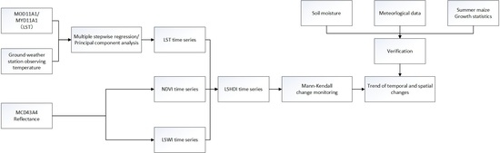
2.3. Construction of the LSHDI

This study was mainly divided into two parts: the construction of temperature time-series data and the construction of LSHDI time-series data. Although the daily MOD11A1 and MYD11A1 land surface temperature products can provide sufficient ground temperature observation data, they are seriously polluted by clouds, which results in the time series of land surface temperature in a particular area being discontinuous. To solve the above problems, this study examined the conversion relationship between MODIS land surface temperature and the measured temperature of the ground weather station. By filling the measured ground temperature into the cloud coverage area in the MODIS ground temperature product, we obtained the final ground temperature time-series data and used them for subsequent heat damage monitoring. Then, this study examined the relationship between the NDVI, LSWI, and LST, and searched for a location with the worst vegetation growth conditions in the three-dimensional feature space constructed by the three variables. Finally, we calculated the distance between each point and this location to measure the degree of vegetation affected by high temperature and heat damage. Figure 2 shows a flowchart that illustrates the method we used, while the main implementation steps are described in detail in the following sections.

2.3.1. Construction of Temperature Time-Series Data

This study used two MODIS surface temperature products (MOD/MYD11A1); therefore, there could be four observations per day for the same pixel. By overlapping the temperature data measured by the ground weather station with two land surface temperature products, each weather station could extract five temperature observations, which were the temperature data obtained by one weather station and four MODIS land surface temperature products. First, we divided all weather stations from 2009 to 2018 into training datasets and test datasets in a 4:1 ratio and ensured that there were observation data for modeling every year to improve the generalization ability of the model [51]. Then, the temperature data obtained by weather station observations were used as the dependent variable, and the ground temperature values obtained from the four daily observations of the two MODIS surface temperature products were used as the independent variables to establish the regression model. Among them, the daytime temperature observation value in the MOD11A1 product is expressed as $T_{OD}$, and the nighttime temperature value is expressed as $T_{ON}$, while the daytime temperature observation value in the MYD11A1 product is expressed as $T_{YD}$, and the nighttime temperature is expressed as $T_{YN}$. This study carried out a correlation test on the above four independent variables and found that the night observation temperatures ($T_{ON}$ and $T_{YN}$) of the two MODIS geothermal products had a significant correlation. After analysis, the correlation coefficient between the two was 0.9650 and reached a significance level of 0.01; therefore, the direct use of the four variables may lead to multicollinearity in the model, and it was necessary to reduce the dimensionality of the independent variables of the model.

There was an obvious linear relationship between the MODIS land surface temperature and the ground weather station temperature [52]. To ensure that the independent variables had a significant impact on the model, this study used a multiple stepwise regression method to gradually introduce the four independent variables into the model. Only one new variable was introduced at a time, and the original variable was tested for significance at the same time. If the original variable was no longer significant, it was removed. In addition, to eliminate the multicollinearity problem caused by the correlation between the independent variables, this study used the principal component analysis method to reduce the dimensions of the four independent variables [53]: $T_{OD}$, $T_{ON}$, $T_{YD}$, and $T_{YN}$. Finally, the extracted principal components were used as new variables in the multiple stepwise regression model. Among them, each variable in the principal component was the original variable obtained by the following standardization process:

$$T_i^{″}=\frac{T_i-T_{min}}{T_{max}-T_{min}}$$

(2)

where $T_i^{″}$ represents the standardized result of the variable, $T_i$ corresponds to the 4 independent variables of land surface temperature, $T_{min}$ represents the lowest temperature in the study area, and $T_{max}$ represents the highest temperature in the study area. To reduce the influence of abnormal values on the standardized results, $T_{min}$ in this study is the temperature value at 0.05% of the lowest temperature cumulative frequency, and $T_{max}$ is the temperature value at 95.5% of the highest temperature cumulative frequency.

This study used this method to unify the four observations of the two kinds of land surface temperature products into one temperature. For the cloudless areas in the MODIS images, this method was used to fit the observation temperature of the ground station. For the areas covered by clouds, the observation data of the ground weather station were used for spatial interpolation, and the interpolation results were filled in the cloud-covered areas to generate more uniform and smooth temperature time-series data. Since the MODIS LST product and the measured data from the ground weather station are both daily observational data, to match the 8-day time resolution of the MCD43A4 land surface reflectance product, this study used the maximum value synthesis method to resample the time resolution of the abovementioned temperature time-series data to 8 days for subsequent research.

2.3.2. Building LSHDI Time-Series Data

Sandholt et al. [18]. found that when the state of the land surface changes from bare to full vegetation cover, the soil moisture also transitions from drought to humid conditions. The distribution of the scattered points in the two-dimensional feature space formed by the NDVI and LST in this area is a triangle, where the two sides of the triangle represent the dry edge and the wet edge, representing the soil moisture state, as shown in Figure 3. The dry edge and the wet edge are defined as in Equation (3).

$$NDVI=\frac{\rho nir-\rho red}{\rho nir+\rho red}$$

(3)

where $\rho nir$ and $\rho red$ represent the reflectance of the image in the near-infrared and red bands, respectively.

$$\begin{array}{c}Dry=a1+b1\ast NDVI\\ Wet=a2+b2\ast NDVI\end{array}$$

(4)

where $Dry$ represents the dry edge, which is the highest LST corresponding to a certain NDVI value, and $Wet$ represents the wet edge, which is the lowest LST corresponding to a certain NDVI value. $a1,b1,a2$, and $b2$ are the coefficients of the dry edge and wet edge fitting equations, respectively.

To determine the relationship between the temperature, moisture, and the growth status of vegetation, this study introduced the LSWI on the basis of the original NDVI–LST two-dimensional feature space and constructed the NDVI–LST–LSWI three-dimensional feature space. This study calculated the characteristics of the scattered point distribution among the NDVI, LSWI, and LST and found that: (1) The scattered point distribution of the NDVI–LSWI two-dimensional feature space was an inverted triangle, similar to the NDVI–LST feature space, and there were also dry edges and wet edges. The two edges that make up the triangle were also closely related to land surface evaporation and vegetation transpiration, and the expression equation can be obtained by fitting scattered points. (2) The distribution of scattered points in the two-dimensional feature space of LSWI–LST was approximately a straight line, which expressed the changing trend of vegetation canopy moisture reduction as the temperature rose. Figure 4 is a schematic diagram of the two-dimensional feature space of NDVI–LSWI and LSWI–LST.

$$LSWI=\frac{\rho nir-\rho swir}{\rho nir+\rho swir}$$

(5)

where $\rho nir$ and $\rho swir (1628-1652 \mathrm{n}\mathrm{m})$ represent the reflectance of the image in the near-infrared and shortwave infrared bands, respectively.

The NDVI reflects the growth of vegetation on the ground, the LSWI reflects the water content of the vegetation canopy, and the LST reflects the temperature environment where the vegetation is located. Both temperature and moisture are very important to the growth of vegetation. In this study, the LST was used as the temperature-influencing factor, the LSWI was used as the moisture-influencing factor, the NDVI was used as the characterization of the vegetation development status, and the three-dimensional feature space of NDVI–LST–LSWI was established. Since in the feature space of NDVI–LST and NDVI–LSWI, the distribution of the scattered points was triangular, and the distribution of the scattered points in the feature space of LSWI–LST was linear, the three-dimensional feature space composed of NDVI–LST–LSWI will also present a spatial triangle, as shown in Figure 5, where ΔABC is the distribution range of these scattered points in the three-dimensional feature space, the AB edge represents the NDVI value, and the BC edge represents the linear feature space of LWSI–LST.

In the three-dimensional feature space composed of NDVI–LST–LSWI, the NDVI and LSWI values at the location of point C were the lowest, and the LST value was the highest, which represents the area with the worst vegetation growth. This location can be expressed as (${NDVI}_{min},{LST}_{max},{LSWI}_{min}$). The coordinates of any point in the spatial characteristic triangle ABC are expressed as (${NDVI}_i,{LST}_i,{LSWI}_i$). The closer the distance to point C is, the worse the growth state of vegetation; that is, the higher the degree of high temperature and heat damage. Therefore, the distance between any point and point C was used as an index to measure the high temperature and heat damage of the crop at that point, which is expressed as Equation (6):

$${Dist}_i=\sqrt{{({NDVI}_i-{NDVI}_{min})}^2+{({LST}_i-{LST}_{max})}^2{+({LSWI}_i-{LSWI}_{min})}^2}$$

(6)

where ${Dist}_i$ represents the Euclidean distance from any point i to the worst point C. In this spatial characteristic triangle, point A represents an area where vegetation is growing well. Its coordinates can be expressed as (${NDVI}_{max},{LST}_{min},{LSWI}_{max}$). In ΔABC, the distance between the two points, A and C, can be expressed as shown in Equation (7):

$${Dist}_{AC}=\sqrt{{({NDVI}_{max}-{NDVI}_{min})}^2+{({LST}_{min}-{LST}_{max})}^2{+({LSWI}_{max}-{LSWI}_{min})}^2}$$

(7)

where ${LST}_{min},{LST}_{max},{LSWI}_{max},\mathrm{a}\mathrm{n}\mathrm{d} {LSWI}_{min}$ are all obtained from the fitting equation of the scattered point distribution in the feature space, as follows:

$$\begin{array}{c}{LST}_{min}=a1+b1\ast {NDVI}_{min}\\ {LST}_{max}=a2+b2\ast {NDVI}_{max}\\ {LSWI}_{min}=a3+b3\ast {NDVI}_{min}\\ {LSWI}_{max}=a4+b4\ast {NDVI}_{max}\end{array}$$

(8)

where $a1,b1,a2,\mathrm{a}\mathrm{n}\mathrm{d} b2$ are the fitting coefficients of the wet and dry edges in the NDVI–LST two-dimensional feature space, $a3,b3,a4,\mathrm{a}\mathrm{n}\mathrm{d} b4$ are the fitting coefficients of the wet and dry edges in the NDVI–LSWI two-dimensional feature space, and ${NDVI}_{min}$ and ${NDVI}_{max}$ are the maximum and minimum values of the NDVI in the study area. Based on the above discussion, this study defines the LSHDI of the land surface vegetation as follows:

$$LSHDI=\frac{{Dist}_i}{{Dist}_{AC}}=\frac{\sqrt{{({NDVI}_i-{NDVI}_{min})}^2+{({LST}_i-{LST}_{max})}^2{+({LSWI}_i-{LSWI}_{min})}^2}}{\sqrt{{({NDVI}_{max}-{NDVI}_{min})}^2+{({LST}_{min}-{LST}_{max})}^2{+({LSWI}_{max}-{LSWI}_{min})}^2}}$$

(9)

where ${LST}_{min},{LST}_{max},{LSWI}_{max},\mathrm{a}\mathrm{n}\mathrm{d} {LSWI}_{min}$ are all obtained by bringing the corresponding maximum or minimum NDVI values into the fitting equation, and the value range of the LSHDI is [0,1]. The LSHDI with 500 m spatial resolution indirectly characterizes the water stress state of the surface vegetation. The smaller the value is, the more serious the water shortage of the vegetation and the higher the degree of high temperature and heat damage; the larger the value is, the more adequate the water supply of the vegetation and the better the growth state of the vegetation.

2.4. Monitoring of High Temperature and Heat Damage of Summer Maize Based on the LSHDI

High temperatures are very harmful to the growth of summer maize, especially in the flowering period of growth, which will eventually affect its yield [54,55]. To monitor the degree of high-temperature heat damage over time, this study used the Mann–Kendall method (MK) to monitor and analyze the impact of high-temperature heat damage on summer maize. The Mann–Kendall method is a commonly used monitoring method in the field of remote sensing [56,57,58,59,60,61,62,63]. It is a nonparametric statistical test method and does not require data to follow a certain mathematical distribution. In addition, it is not sensitive to outliers and is suitable for time-series analysis [56]. This method can not only obtain the trend of the time series but can also detect mutation points [57,58,59,60,61,62,63].

2.4.1. Mann–Kendall Trend Monitoring

For the time series X, the Mann–Kendall method defines the statistic S as:

$$S={\sum }_{i=2}^n{\sum }_{j=1}^{i-1}(X_i-X_j)$$

(10)

where $X_i$ and $X_j$ represent the i-th and j-th values of the time series, respectively, n represents the number of observations in the time series, and the value of $(X_i-X_j)$ is determined by the positive and negative conditions of the results. For example, when $(X_i-X_j)$ is greater than, equal to, or less than 0, its value is −1, 0, and 1, respectively. At this time, the statistic Z is defined as:

$$\begin{array}{cc}●\hspace{1em}Z=\frac{S-1}{\sqrt{\frac{n(n-1)(2n+5)}{18}}}& \hspace{1em}\hspace{1em}\hspace{1em}\mathrm{S}>0\\ ●\hspace{1em}Z=0& \hspace{1em}\hspace{1em}\hspace{1em}\mathrm{S}=0\\ ●\hspace{1em}Z=\frac{S+1}{\sqrt{\frac{n(n-1)(2n+5)}{18}}}& \hspace{1em}\hspace{1em}\hspace{1em}\mathrm{S}<0\end{array}$$

(11)

The statistic Z is used to describe the trend of the time series X. When Z is greater than 0, the time series shows an increasing trend; when Z is less than 0, the time series shows a decreasing trend [63]. In addition, the larger the absolute value of Z is, the more obvious the trend of change.

2.4.2. Mann–Kendall Mutation Detection

For a time series, X, containing n samples, the Mann–Kendall method constructs the order sequence, $S_k$, as:

$$S_k=\sum _{i=1}^k{r}_i (\mathrm{k}=2,3,\dots ,\mathrm{n})$$

(12)

When $X_i>X_j$, the value of $r_i$ is 1; otherwise, it is 0; that is, the sequence column $S_k$ represents the number of values at the i-th moment greater than the value at the j-th moment. At this time, the statistic ${UF}_k$ is defined as:

$${UF}_k=\frac{S_k-E\left(S_k\right)}{\sqrt{Var\left(S_k\right)}}$$

(13)

where $E\left(S_k\right)$ is the mean value of the sequence $S_k$, and $Var\left(S_k\right)$ is the variance of the sequence, and their values are:

$$\begin{array}{c}●\hspace{1em}E(S_k)=\frac{n(n+1)}{4}\\ ●\hspace{1em}Var(S_k)=\frac{n(n-1)(2n+5)}{72}\end{array}$$

(14)

At this moment, the inverse sequence of the time series X ($X_n,X_{n-1},X_{n-2},\dots ,X_1$) is repeatedly calculated to obtain the statistic ${UB}_k$. If the values of ${UF}_k$ and ${UB}_k$ are greater than 0, it indicates that the time series shows an upward trend, and if the values are less than 0, it indicates a descending trend. When the two curves of ${UF}_k$ and ${UB}_k$ intersect, the moment corresponding to the intersection is the mutation point [64].

The use of the Mann–Kendall method for trend monitoring and mutation detection is not only simple in calculation but also has significant results. This study used this method to perform trend analysis and mutation point detection on the LSHDI time series of the Huanghuaihai Plain. Finally, the combination of soil moisture and climate data can serve as a reference to explain the abovementioned temporal and spatial changes. Figure 6 shows a flowchart that illustrates this process.

3. Results

3.1. Performance of the LSHDI

Since MODIS data have a rich number of bands and each of the bands have been widely used and quality-verified, this study first used MODIS LST time-series data and MCD43A4 data to examine the construction method of the LSHDI at coarser spatial resolutions.

3.1.1. Construction and Verification of Temperature Time-Series Data

This study used multiple stepwise regression combined with principal component analysis, and the three principal components obtained were as follows:

$$●\hspace{1em}{X}_1=0.499T_{OD}^{″}+0.520T_{ON}^{″}+0.464T_{YD}^{″}+0.514T_{YN}^{″}$$

(15)

$$●\hspace{1em}{X}_2=0.284T_{OD}^{″}-0.438T_{ON}^{″}+0.709T_{YD}^{″}-0.472T_{YN}^{″}$$

(16)

$$●\hspace{1em}{X}_3=-0.816T_{OD}^{″}+1.069T_{ON}^{″}+0.530T_{YD}^{″}+0.205T_{YN}^{″}$$

(17)

where $X_1$, $X_2$, and $X_3$ represent the three linearly independent principal components, and $T_{OD}^{″}$, $T_{ON}^{″}$, $T_{YD}^{″}$, and $T_{YN}^{″}$ represent the four kinds of LST variables standardized by Equation (2). We used the above three principal components as new variables to perform multiple stepwise regression again, and then restored them to the initial variables and obtained the linear regression model as follows:

$$\mathrm{Y}=0.085T_{OD}+0.444T_{ON}+0.176T_{YD}+0.323T_{YN}+0.299$$

(18)

where Y represents the temperature data observed by the ground weather station, and $T_{OD}$, $T_{ON}$, $T_{YD}$, and $T_{YN}$ represent the four time pixel values observed in the MODIS land surface temperature product. The collinearity test of the model established by Equation (16) shows that there was no multicollinearity.

Considering that the performance of the model is slightly different in plain and mountainous areas, this study separately examined them. Figure 7 shows the relationship between the simulated temperature value Y of the model and the ground-measured temperature (validation data). The scattered points were evenly distributed on both sides of the 1:1 line. The model determination coefficient (R2) in the plain area was 0.8202, and the root mean square error (RMSE) was 1.28 °C. The model determination coefficient (R2) in mountainous areas was 0.8109, and the root mean square error (RMSE) was 2.32 °C. Both reached the 0.001 significance level.

In summary, the model had good simulation accuracy, and the simulation accuracy in plain areas was slightly higher than that in mountainous areas. This is inseparable from the complexity and change in mountainous terrain. The accuracy is consistent with the existing published research results [65,66]. The LST time series during the high-temperature-sensitive period (DOY = 185–241) of summer maize on the Huanghuaihai Plain in 2018 is shown in Figure 8.

3.1.2. Performance of the LSHDI under Coarse Spatial Resolution

This study used MCD43A4 (DOY = 185–241) in 2018 to calculate the NDVI and LSWI according to Equations (3) and (5), respectively. Figure 9 shows the time series of the NDVI and LSWI.

Based on the NDVI, LSWI, and LST datasets during the high-temperature- and heat-damage-sensitive periods of summer maize in 2018, we counted and plotted the scattered point distribution in its feature space, as shown in Figure 10 (the sign “*” in figure body mean Multiplication). Among them, Figure 10a,d,g,j,m,p,s,v represent the NDVI–LST two-dimensional feature space scatter point distributions; Figure 10b,e,h,k,n,q,t,w represent the NDVI–LSWI two-dimensional feature space scatter point distributions; and Figure 10c,f,i,l,o,r,u,x represent the LSWI–LST two-dimensional feature space scatter point distributions.

The LSHDI time series in 2018 (DOY = 185–241), calculated according to Section 2.3.2, is shown in Figure 11.

The red area in the figure represents the area that suffers from high temperature and heat damage, and the blue–green area indicates that the vegetation in this area is growing well. There are a total of 552 soil moisture sites in this area, which were used to record the relative soil moisture content. Since the soil moisture at a surface depth of 10–20 cm is relatively stable, the data at this depth were selected as a reference for the spatial distribution trend of the abovementioned eight phases of the index. The results show that the LSHDI had a good correlation with soil moisture, and the two were scattered. The coefficients of determination of the fitted models of the distribution were all above 0.5 and reached a significance level of 0.01, as shown in Figure 12.

3.1.3. Sensitivity Analysis of Factors in the LSHDI

Based on the above discussion, we separately counted the correlation between the NDVI/LSWI/LST and the LSHDI. The results show that the correlation between the former three and the LSHDI was not much different, and the correlation between the LST and the LSHDI was slightly higher: their coefficient of determination reached 0.6383, as shown in Figure 13.

We conducted a sensitivity analysis on the three factors, NDVI, LSWI, and LST, and found that the results were consistent with the above results. Both the first-order sensitivity and the total-order sensitivity of LST were higher than those of the other two factors, which shows that the surface temperature contributed the most to the LSHDI (see Figure 14).

3.2. Temporal and Spatial Changes in Heat Damage in Summer Maize on the Huanghuaihai Plain

In this study, the Mann–Kendall method was used to monitor the changes in the LSHDI during and between years. We studied the spatial trend of the index and its significance, and based on this, we summarized the frequency and time of high-temperature and heat damage events in the main production areas of Huanghuaihai summer maize.

3.2.1. Trend of the LSHDI during the Year

According to the disaster statistics released by the National Meteorological Center, 2018 was the year when summer maize in Huanghuaihai was more severely affected. This study took the LSHDI time series from July to August 2018 (Figure 11) as the key research object. After the Mann–Kendall spatial trend test, the results are shown in Figure 15. The LSHDI presented a clear trend of change, among which the eastern region presented a relatively obvious upward trend of the index; that is, as the season passed, the high-temperature period gradually transitioned, and the vegetation growth state tended to improve. The western region showed an obvious downward index trend, the growth status of vegetation deteriorated, and the high temperature caused irreversible damage to the vegetation.

Soil moisture can reflect the damage to vegetation affected by temperature and water, and there is no reliable disaster verification dataset that has been published at present; therefore, this study used soil moisture data as a reference for spatial change trends. The results are shown in Figure 16. The larger point in Figure 16a represents an increasing trend in the time series of soil moisture; that is, an increase in soil moisture. A smaller point represents a downward trend in the time series of soil moisture; that is, a decrease in soil moisture. The spatial trend of soil moisture is in good agreement with the spatial trend of the LSHDI. The coefficient of determination of the fitting equation of the two scattered point distributions was 0.9483, and it passed the p < 0.001 significance test, indicating a good correlation between the LSHDI and soil moisture. The use of the LSHDI to monitor land surface water or conduct vegetation high temperature and heat damage has higher accuracy and better application prospects.

During the flowering stage of summer maize growth, high temperature and heat damage may occur more than once, and multiple mutation points may be detected by the MK mutation test method. These mutation points may represent a mutation of the vegetation status from good to bad, or they may represent a mutation of the vegetation status from bad to good. Therefore, this study combined the trend of the LSHDI time series, and after the second screening of the detected mutation points, the mutation points that characterize the vegetation status from bad to good, that is, the moment of high temperature and heat damage, were obtained. We counted the frequency of high-temperature heat damage in this area, as shown in Figure 17.

Figure 17 shows the frequency of high-temperature and heat damage events and their distribution in summer maize. Figure 17a shows the frequency of high-temperature heat damage events, Figure 17b shows the distribution of the period of the first heat damage event when one or more heat damage events occurred, Figure 17c shows the distribution of the period of the second heat damage when two or more heat damage events occurred, and Figure 17d shows the distribution of the second heat damage event when three or more heat damage events occurred. In the main production area of Huanghuaihai summer maize in 2018, a large area had one high-temperature and high-heat damage event. There were two heat damage events in southern Hebei Province and northern and eastern Henan Province. The three heat damage events only occurred in a few areas. In addition, the period of one heat damage event occurred mostly in early July (Day of the year (DOY) = 185–193), and in parts of southern Shanxi Province and southern Henan Province, it occurred in early August (DOY = 217–225). The regional distribution of the second high-temperature and heat damage event was relatively wide and uniform, and the period occurred in middle and late August (DOY = 225–233). The period of the third heat damage event occurred at the end of August (DOY = 233–241).

This study also used the soil moisture time series at the same time to perform the MK mutation test and used the confusion matrix to calculate the overall accuracy and Kappa coefficient to characterize the accuracy of the results. Figure 18 shows the frequency of mutations of soil moisture on the Huanghuaihai Plain during the flowering period of summer maize in 2018. The larger the point is, the higher the frequency of mutations. Figure 18a shows the confusion matrix of the LSHDI and the frequency monitoring results of soil moisture. It was calculated that the overall accuracy of the frequency monitoring of high-temperature heat damage using the LSHDI was 95.54%, and the Kappa coefficient was 0.8944, which is consistent with the measured soil moisture data. Figure 18b,c show the distribution histograms of the LSHDI and soil moisture frequency monitoring results of thermal events. Figure 19 shows the percentage of misclassifications in the LSHDI monitoring results.

3.2.2. Trend of the LSHDI between Years

To study the interannual variation in high temperature and heat damage in the main production areas of Huanghuaihai summer maize, this study obtained MCD43A4 land surface reflectance data from 2009 to 2018 and produced the LSHDI time-series dataset for each year in this area. The smaller the LSHDI value is, the more severe the area suffers from high temperature and heat damage. This study combined the 8 LSHDI datasets of each year with the minimum value, and finally, obtained the interannual time series of 10 LSHDI scenarios, as shown in Figure 20. The results show that the high temperature and heat damage suffered by the Huanghuaihai Plain first decreased and then increased. Among them, 2010–2011 and 2017–2018 both suffered more severe high temperature and heat damage, and approximately around 2013 was the best period for the growth of crops. According to the global climate change report, relevant climate statistics, and references, the global climate showed a trend of improvement from 2010 to 2015, and there were many extreme weather events in approximately 2018. The trend of the results was consistent.

According to the “Agricultural Drought Grading” standard issued by the National Standardization Administration of China in 2015, when the soil moisture is between 50% and 60%, it is defined as light drought; when it is between 40% and 50%, it is defined as medium drought; when it is between 30% and 40%, it is defined as severe drought, and when it is less than 30%, it is defined as extreme drought [67]. This study analyzed the correspondence between all soil moisture levels and the LSHDI from 2009 to 2018, transformed the above classification system into the value of the LSHDI (as shown in

Table 1. High-temperature heat damage level.

Level	Relative Humidity of the Soil (%)	LSHDI
Light	50~60	Level-1: 0.3~0.4
Moderate	40~50	Level-2: 0.3~0.2
Heavy	30~40	Level-3: 0.2~0.1
Extreme	<30	Level-4: <0.1

), and finally, obtained the 2009–2018 Huanghuaihai Plain results. The distribution of disaster areas is shown in Figure 21. The results show that the area affected by high-temperature heat damage first decreased and then increased with time, while the spatial distribution of areas where high-temperature heat damage occurred was quite different; that is, it had greater spatial variability. In Shanxi Province and the southern part of Shaanxi Province, there have been high-temperature and heat damage events for many years. Finally, the annual disaster area was compared with the annual output of summer corn released by the National Bureau of Statistics. The results show that the high-temperature and heat damage area and the corn yield were obviously negatively correlated. As the disaster area increased, the crop yield significantly decreased, as shown in Figure 22.

The spatial trend of the LSHDI of the Huanghuaihai Plain from 2009 to 2018 is shown in Figure 23. The results show that the boundaries of the spatial trend of heat damage were in a high degree of agreement with the boundaries of administrative divisions. Therefore, there are certain differences in planting habits or planting methods in various provinces. Since most of the study area is a plain area with an altitude of less than 50 m, this phenomenon may be caused by differences in crop cultivation and irrigation methods in different areas after excluding topographic factors. From 2009 to 2018, Hebei Province, northern Anhui Province, and southern Shaanxi Province showed an obvious trend of increasing damage. Central Henan Province, southern Shanxi Province, and Shandong Province showed a trend of good crop growth. We converted the daily minimum soil moisture observation data into an interannual scale and used the MK method to perform the same trend and mutation detection, which can be a stable reference to explain the abovementioned trend monitoring results. The interannual spatial trend of soil moisture is shown in the figure. As shown in Figure 24a, larger points indicate a good direction of change, and smaller points indicate a direction of poor change. The interannual monitoring results based on the LSHDI were very similar to the interannual monitoring results based on soil moisture. They have good agreement, the coefficient of determination between the two was as high as 0.9060, and they passed the p < 0.001 significance test, as shown in Figure 24b.

Figure 25 shows the frequency of high-temperature thermal damage in this area from 2009 to 2018. Figure 25a shows the frequency of heat damage based on the LSHDI, Figure 25b shows the frequency of heat damage based on soil moisture, and Figure 25c–f show the periods of high-temperature and heat damage events of each frequency. The above results show that high-temperature and heat damage events occurred in most regions from 2009 to 2018, with a minimum frequency of 1 and a maximum of 4, and high-frequency heat damage events occurred in southern Hebei Province, central Henan Province, and Anhui Province.

The MK mutation test was performed using the interannual time series of soil moisture at the same time as a reference to explain the above monitoring results, and the confusion matrix was used to calculate the overall accuracy and the accuracy of the Kappa coefficient characterization results. Figure 26a shows the confusion matrix of the frequency monitoring results of the LSHDI and the soil moisture. From this, it was calculated that the overall accuracy of the frequency monitoring of high temperature and thermal damage using the LSHDI was 80.87% and the Kappa coefficient was 0.7132, as shown in Figure 26b,c, respectively, showing the distribution histograms of the LSHDI and soil moisture monitoring results of the thermal event frequency. Figure 27 shows the proportion of misclassifications in the LSHDI monitoring results.

Since the actual area of summer maize suffering from high temperature and heat damage is difficult to count, there is no publicly released dataset of crop damage statistics with high accuracy; therefore, this study verified the monitoring results through relevant statistical data. According to the National Meteorological Center’s agricultural meteorological information products and related journal news, a wide range of extreme high-temperature weather exceeding 35 °C occurred in Hebei, Henan, and Shandong Provinces for more than 10 consecutive days from July to August 2017. The highest value was reached during the same period in 1981–2018, and the high-temperature period is also consistent with the flowering period of summer maize growth. We combined the results with the summer maize yield reduction rate calculated by the National Statistical Yearbook, and we inferred that a relatively serious high temperature and heat did occur during this period.

4. Discussion

Traditional crop heat damage monitoring technology based on point source data cannot represent the surface environmental conditions of a large area. This study used high-temporal-resolution data to construct the LSHDI to solve the above contradiction. The traditional vegetation monitoring based on a particular remote sensing index only analyzes the growth state or temporal and spatial trends of the surface vegetation from a single aspect, and these results can reflect the vegetation’s current state one-sidedly, but cannot accurately reflect its overall development and the environment in which it is located. This study combined the LST, NDVI, and LSWI to build the LSHDI, which more comprehensively reflects the growth of vegetation and its living environment. The index not only takes into account the visual observation of vegetation growth but also considers the temperature and humidity environment of vegetation and improves the accuracy of monitoring results. The remote sensing data and ground observation data are effectively combined to better derive the vegetation changes in the study area. For crop thermal-damage monitoring, one of the most critical problems at present is the lack of valid verification data. At present, most studies have been based on soil moisture, which indirectly reflects the damage to vegetation [68,69,70]. This study is no exception. Although the LSHDI comprehensively reflects the growth of vegetation and the state of the environment in terms of vegetation growth, temperature, and moisture, the correlation between the index and soil moisture is still not very strong. Furthermore, the LST, NDVI, and LSWI used in this study are only some of the many indices reflecting surface temperature, vegetation growth, and surface moisture, respectively. In fact, there are still many other indices that can be used in place of these three major indices. This research did not study the relationship between these indices in depth. This study used MODIS data to conduct a large-scale, high-temperature heat damage monitoring study on the Huanghuaihai Plain. Finally, the detection method for the trend and sudden change of the high-temperature heat damage index time series can be further optimized because the traditional Mann–Kendall monitoring method used in this study loses information and cannot capture the subtle changes in the time series.

In addition, the use of time-series data with high temporal resolution also has some unsolved problems. The index product with coarser spatial resolution can characterize the overall trend of the area and generally has temporal continuity. However, due to the existence of mixed pixels, the value of a certain pixel in the product represents the comprehensive contribution of various surrounding ground objects, which obscures the spatial details, and navigation has poor interpretation of the monitoring results or even cannot explain it [71,72,73,74,75]. This effect is often more obvious on images with coarser spatial resolution. The use of index products with higher spatial resolution for monitoring research could solve this problem. First, higher spatial resolution adds more spatial detail information to the monitoring results, and the clearer land surface coverage makes the abovementioned inexplicable changes well-founded. Second, data with higher spatial resolution can weaken the influence of mixed pixels to a greater extent. The higher the spatial resolution is, the closer the pixel value will be to the true land surface state. Finally, the use of time-series remote sensing data with high spatial and temporal resolution for monitoring research not only inherits the time continuity advantages of products with coarser spatial resolution but also makes the monitoring results clearer and more uniform in the performance of spatial changes with more spatial details. These shortcomings are also an important improvement direction for the future use of high temporal and spatial resolution time-series data to monitor land surface changes [76,77]. In summary, for different monitoring needs and accuracy requirements, users are required to make a trade-off between spatial details and calculation efficiency in accordance with the actual situation and select remote sensing data with an appropriate resolution.

5. Conclusions

This study combined vegetation greenness, temperature, and soil moisture to construct the LSHDI to monitor the impact to vegetation from high temperature and heat damage. We took summer maize on the Huanghuaihai Plain as the research object and monitored the annual and interannual changes in summer maize damaged by high temperature and heat. To ensure the continuity of temporal and spatial temperature data, this study utilized a method to construct temperature time series. This method uses a combination of multiple stepwise regression and principal component analysis to combine MODIS land surface temperature products with ground temperature observation data and generates a cloud-free temperature time-series dataset.

Based on the temperature time-series dataset, the NDVI time-series dataset, and the LSWI time-series dataset, this study first carried out the construction and application of the LSHDI under the high temporal resolution data of MODIS. The results showed that the coefficient of determination of the fitting model between soil moisture and the LSHDI was above 0.5, and it passed the p < 0.01 significance test. Then, we used the Mann–Kendall method to monitor the interannual and inter-seasonal changes in the long-term LSHDI dataset of the Huanghuaihai summer maize-planting area. The results showed that: (1) The area affected by high temperature and heat damage on the Huanghuaihai Plain showed a decrease first and then an increase from 2009 to 2018. Among them, 2010, 2017, and 2018 suffered severe high-temperature heat damage. (2) High temperature and heat damage occurred in most of Hebei Province, southeastern Henan Province, southern Shaanxi Province, and parts of northern Anhui Province. (3) In the past ten years, the frequency of high-temperature heat damage on the Huanghuaihai Plain was at least one time, and at most four times, and only one or two high-temperature heat damage events occurred in most areas. (4) Among the more severely affected years, the heat damage was the most severe in late July and early August, the flowering period of summer maize, which had a greater impact on the final yield. (5) Climatic factors such as precipitation can effectively alleviate the damage of high temperatures on summer maize. Finally, we presented soil moisture data as a stable reference to explain the results of the trend analysis, and the coefficient of determination between them was above 0.9 and reached a significance level of 0.001.

References

1. Ryu, J.H.; Oh, D.; Ko, J.; Kim, H.Y.; Yeom, J.M.; Cho, J. Remote Sensing-Based Evaluation of Heat Stress Damage on Paddy Rice Using NDVI and PRI Measured at Leaf and Canopy Scales. Agronomy 2022, 12, 1972. [Google Scholar] [CrossRef]
2. Gong, L.; Li, X.; Tian, B.; Wang, P.; Jiang, L.; Zhao, H. Spatio-temporal characteristics of drought in different growth stages of soybean in Heilongjiang. J. Appl. Meteor. Sci. 2020, 31, 95–104. [Google Scholar]
3. Yang, J.; Huo, Z.; Wang, P.; Wu, D. Occurrence characteristics of early rice heat disaster in Jiangxi Province. J. Appl. Meteor. Sci. 2020, 31, 42–51. [Google Scholar]
4. Dou, Y.; Huang, R.; Mansaray, L.R.; Huang, J. Mapping high temperature damaged area of paddy rice along the Yangtze River using Moderate Resolution Imaging Spectroradiometer data. Int. J. Remote Sens. 2019, 41, 471–486. [Google Scholar] [CrossRef]
5. Dai, A. Drought under global warming: A review. Wiley Interdiscip. Rev. Clim. Chang. 2011, 2, 45–65. [Google Scholar] [CrossRef]
6. Palmer, W.C. Meteorological Drought; US Department of Commerce, Weather Bureau: Washington, DC, USA, 1965.
7. Vicente-Serrano, S.M.; Beguería, S.; López-Moreno, J.I. A Multiscalar Drought Index Sensitive to Global Warming: The Standardized Precipitation Evapotranspiration Index. J. Clim. 2010, 23, 1696–1718. [Google Scholar] [CrossRef]
8. Johnson, W.K.; Kohne, R.W. Susceptibility of Reservoirs to Drought Using Palmer Index. J. Water Resour. Plan. Manag. 1993, 119, 367–387. [Google Scholar] [CrossRef]
9. Bian, Z.; Roujean, J.L.; Fan, T.; Dong, Y.; Hu, T.; Cao, B.; Li, H.; Du, Y.; Xiao, Q.; Liu, Q. An angular normalization method for temperature vegetation dryness index (TVDI) in monitoring agricultural drought. Remote Sens. Environ. 2023, 284, 113330. [Google Scholar] [CrossRef]
10. Kogan, F. Application of vegetation index and brightness temperature for drought detection. Adv. Space Res. 1995, 15, 91–100. [Google Scholar] [CrossRef]
11. Sun, H.; Chen, Y.; Sun, H. Comparisons and classification system of typical remote sensing indexes for agricultural drought. Trans. Chin. Soc. Agric. Eng. 2012, 28, 147–154. [Google Scholar]
12. Wen, Q.; Sun, P.; Zhang, Q.; Liu, J.; Shi, P. An integrated agricultural drought monitoring model based on multi-source remote sensing data: Model development and application. Acta Ecol. Sin. 2019, 39, 7757–7770. [Google Scholar]
13. Tucker, C.J.; Choudhury, B.J. Satellite remote sensing of drought conditions. Remote Sens. Environ. 1987, 23, 243–251. [Google Scholar] [CrossRef]
14. Ji, L.; Peters, A.J. Assessing vegetation response to drought in the northern Great Plains using vegetation and drought indices. Remote Sens. Environ. 2003, 87, 85–98. [Google Scholar] [CrossRef]
15. Boschetti, M.; Nutini, F.; Brivio, P.A.; Bartholomé, E.; Stroppiana, D.; Hoscilo, A. Identification of environmental anomaly hot spots in West Africa from time series of NDVI and rainfall. ISPRS J. Photogramm. Remote Sens. 2013, 78, 26–40. [Google Scholar] [CrossRef]
16. Liu, L.; Yang, X.; Gong, F.; Su, Y.; Huang, G.; Chen, X. The Novel Microwave Temperature Vegetation Drought Index (MTVDI) Captures Canopy Seasonality across Amazonian Tropical Evergreen Forests. Remote Sens. 2021, 13, 339. [Google Scholar] [CrossRef]
17. Kogan, F. World droughts in the new millennium from AVHRR-based vegetation health indices. Eos 2002, 83, 557–563. [Google Scholar] [CrossRef]
18. Sandholt, I.; Rasmussen, K.; Andersen, J. A simple interpretation of the surface temperature/vegetation index space for assessment of surface moisture status. Remote Sens. Environ. 2002, 79, 213–224. [Google Scholar] [CrossRef]
19. Patel, N.R.; Parida, B.R.; Venus, V.; Saha, S.K.; Dadhwal, V.K. Analysis of agricultural drought using vegetation temperature condition index (VTCI) from Terra/MODIS satellite data. Environ. Monit. Assess. 2011, 184, 7153–7163. [Google Scholar] [CrossRef]
20. Zhou, X.; Wang, P.; Tansey, K.; Zhang, S.; Li, H.; Wang, L. Developing a fused vegetation temperature condition index for drought monitoring at field scales using Sentinel-2 and MODIS imagery. Comput. Electron. Agric. 2020, 168, 105144. [Google Scholar] [CrossRef]
21. Basak, A.; Rahman, A.S.; Das, J.; Hosono, T.; Kisi, O. Drought forecasting using the Prophet model in a semi-arid climate region of western India. Hydrol. Sci. J. 2022, 67, 1397–1417. [Google Scholar] [CrossRef]
22. Zhou, X.; Wang, P.; Tansey, K.; Ghent, D.; Zhang, S.; Li, H.; Wang, L. Drought Monitoring Using the Sentinel-3-Based Multiyear Vegetation Temperature Condition Index in the Guanzhong Plain, China. IEEE J. Sel. Top. Appl. Earth Obs. Remote Sens. 2019, 13, 129–142. [Google Scholar] [CrossRef]
23. Viswambharan, S.; Kumaramkandath, I.T.; Tali, J.A. A geospatial approach in monitoring the variations on surface soil moisture and vegetation water content: A case study of Palakkad District, Kerala, India. Environ. Earth Sci. 2022, 81, 494. [Google Scholar] [CrossRef]
24. Xu, Y.; Gao, C.; Li, X.; Yang, T.; Sun, X.; Wang, C. The Design of a Drought Weather Index In-surance System for Summer Maize in Anhui Province, China. J. Risk Anal. Crisis Response (JRACR) 2018, 8, 14. [Google Scholar] [CrossRef]
25. Li, M.; Liu, M.; Liu, X.; Peng, T.; Wang, S. Decomposition of long time-series fraction of absorbed photo-synthetically active radiation signal for distinguishing heavy metal stress in rice. Comput. Electron. Agric. 2022, 198, 107111. [Google Scholar] [CrossRef]
26. Crusiol, L.G.T.; Sun, L.; Sun, Z.; Chen, R.; Wu, Y.; Ma, J.; Song, C. In-Season Monitoring of Maize Leaf Water Content Using Ground-Based and UAV-Based Hyperspectral Data. Sustainability 2022, 14, 9039. [Google Scholar] [CrossRef]
27. Ndlovu, H.S.; Odindi, J.; Sibanda, M.; Mutanga, O.; Clulow, A.; Chimonyo, V.G.; Mabhaudhi, T. A Comparative Estimation of Maize Leaf Water Content Using Machine Learning Techniques and Unmanned Aerial Vehicle (UAV)-Based Proximal and Remotely Sensed Data. Remote Sens. 2021, 13, 4091. [Google Scholar] [CrossRef]
28. Zheng, Y.; Xiao, Z.; Li, J.; Yang, H.; Song, J. Evaluation of Global Fraction of Absorbed Photosynthetically Active Radiation (FAPAR) Products at 500 m Spatial Resolution. Remote Sens. 2022, 14, 3304. [Google Scholar] [CrossRef]
29. Xiao, Z.; Liang, S.; Sun, R. Evaluation of Three Long Time Series for Global Fraction of Absorbed Photosynthetically Active Radiation (FAPAR) Products. IEEE Trans. Geosci. Remote Sens. 2018, 56, 5509–5524. [Google Scholar] [CrossRef]
30. Tao, X.; Liang, S.; He, T.; Jin, H. Estimation of fraction of absorbed photosynthetically active radiation from multiple satellite data: Model development and validation. Remote Sens. Environ. 2016, 184, 539–557. [Google Scholar] [CrossRef]
31. Yang, Z.L.; Zhang, T.B.; Yi, G.H.; Li, J.J.; Qin, Y.B.; Chen, Y. Erratum to: Spatio-temporal variation of Fraction of Photosynthetically Active Radiation absorbed by vegetation in the Hengduan Mountains, China. J. Mt. Sci. 2021, 18, 1710. [Google Scholar] [CrossRef]
32. Mahanand, S.; Behera, M.D.; Roy, P.S.; Kumar, P.; Barik, S.K.; Srivastava, P.K. Satellite Based Fraction of Absorbed Photosynthetically Active Radiation Is Congruent with Plant Diversity in India. Remote Sens. 2021, 13, 159. [Google Scholar] [CrossRef]
33. Peng, D.; Zhang, H.; Yu, L.; Wu, M.; Wang, F.; Huang, W.; Liu, L.; Sun, R.; Li, C.; Wang, D.; et al. Assessing spectral indices to estimate the fraction of photosynthetically active radiation absorbed by the vegetation canopy. Int. J. Remote Sens. 2018, 39, 8022–8040. [Google Scholar] [CrossRef]
34. Chatterjee, S.; Desai, A.R.; Zhu, J.; Townsend, P.A.; Huang, J. Soil moisture as an essential component for delineating and forecasting agricultural rather than meteorological drought. Remote Sens. Environ. 2022, 269, 112833. [Google Scholar] [CrossRef]
35. Kowalski, K.; Okujeni, A.; Brell, M.; Hostert, P. Quantifying drought effects in Central European grasslands through regression-based unmixing of intra-annual Sentinel-2 time series. Remote Sens. Environ. 2022, 268, 112781. [Google Scholar] [CrossRef]
36. Jiao, W.; Wang, L.; McCabe, M.F. Multi-sensor remote sensing for drought characterization: Current status, opportunities and a roadmap for the future. Remote Sens. Environ. 2021, 256, 112313. [Google Scholar] [CrossRef]
37. von Keyserlingk, J.; de Hoop, M.; Mayor, A.; Dekker, S.; Rietkerk, M.; Foerster, S. Resilience of vegetation to drought: Studying the effect of grazing in a Mediterranean rangeland using satellite time series. Remote Sens. Environ. 2021, 255, 112270. [Google Scholar] [CrossRef]
38. Souza, A.G.S.S.; Neto, A.R.; de Souza, L.L. Soil moisture-based index for agricultural drought assessment: SMADI application in Pernambuco State-Brazil. Remote Sens. Environ. 2021, 252, 112124. [Google Scholar] [CrossRef]
39. Xu, L.; Abbaszadeh, P.; Moradkhani, H.; Chen, N.; Zhang, X. Continental drought monitoring using satellite soil moisture, data assimilation and an integrated drought index. Remote Sens. Environ. 2020, 250, 112028. [Google Scholar] [CrossRef]
40. West, H.; Quinn, N.; Horswell, M. Remote sensing for drought monitoring & impact assessment: Progress, past challenges and future opportunities. Remote Sens. Environ. 2019, 232, 111291. [Google Scholar] [CrossRef]
41. Wang, Q.; Zhao, L.; Wang, M.; Wu, J.; Zhou, W.; Zhang, Q.; Deng, M. A Random Forest Model for Drought: Monitoring and Validation for Grassland Drought Based on Multi-Source Remote Sensing Data. Remote Sens. 2022, 14, 4981. [Google Scholar] [CrossRef]
42. Bhardwaj, J.; Kuleshov, Y.; Chua, Z.W.; Watkins, A.B.; Choy, S.; Sun, Q. Evaluating Satellite Soil Moisture Datasets for Drought Monitoring in Australia and the South-West Pacific. Remote Sens. 2022, 14, 3971. [Google Scholar] [CrossRef]
43. Zhou, H.; Geng, G.; Yang, J.; Hu, H.; Sheng, L.; Lou, W. Improving Soil Moisture Estimation via Assimilation of Remote Sensing Product into the DSSAT Crop Model and Its Effect on Agricultural Drought Monitoring. Remote Sens. 2022, 14, 3187. [Google Scholar] [CrossRef]
44. Qureshi, S.; Koohpayma, J.; Firozjaei, M.K.; Kakroodi, A.A. Evaluation of Seasonal, Drought, and Wet Condition Effects on Performance of Satellite-Based Precipitation Data over Different Climatic Conditions in Iran. Remote Sens. 2021, 14, 76. [Google Scholar] [CrossRef]
45. Páscoa, P.; Gouveia, C.M.; Russo, A.C.; Bojariu, R.; Vicente-Serrano, S.M.; Trigo, R.M. Drought Impacts on Vegetation in Southeastern Europe. Remote Sens. 2020, 12, 2156. [Google Scholar] [CrossRef]
46. Filgueiras, R.; Almeida, T.S.; Mantovani, E.C.; Dias, S.H.B.; Fernandes-Filho, E.I.; da Cunha, F.F.; Venancio, L.P. Soil water content and actual evapotranspiration pre-dictions using regression algorithms and remote sensing data. Agric. Water Manag. 2020, 241, 106346. [Google Scholar] [CrossRef]
47. Zhao, H.; Chen, X.; Yang, J.; Yao, C.; Zhang, Q.; Mei, P. Comprehensive Assessment and Variation Characteristics of the Drought Intensity in North China Based on EID. J. Appl. Meteorol. Clim. 2022, 61, 297–308. [Google Scholar] [CrossRef]
48. Chen, H.; Liu, Y.; Du, Z.; Liu, Z.; Zou, C. The change of growing season of the vegetation in Huanghe-Huaihe-Haihe Region and its responses to climate changes. J. Appl. Meteor. Sci. 2011, 22, 437–444. [Google Scholar]
49. Schaaf, C.B.; Gao, F.; Strahler, A.H.; Lucht, W.; Li, X.; Tsang, T.; Strugnell, N.C.; Zhang, X.; Jin, Y.; Muller, J.-P.; et al. First operational BRDF, albedo nadir reflectance products from MODIS. Remote Sens. Environ. 2002, 83, 135–148. [Google Scholar] [CrossRef]
50. Wan, Z.; Dozier, J. A generalized split-window algorithm for retrieving land-surface temperature from space. IEEE Trans. Geosci. Remote Sens. 1996, 34, 892–905. [Google Scholar] [CrossRef]
51. Yang, L.; Han, L.; Song, J.; Li, S. Monitoring and evaluation of high temperature and heat damage of summer maize based on remote sensing data. J. Appl. Meteor. Sci. 2020, 31, 749–758. [Google Scholar]
52. Sohrabinia, M.; Zawar-Reza, P.; Rack, W. Spatio-temporal analysis of the relationship between LST from MODIS and air temperature in New Zealand. Theor. Appl. Climatol. 2015, 119, 567–583. [Google Scholar] [CrossRef]
53. Eduk, A.R. Prediction and Modeling of Dry Seasons Air pollution changes using multiple linear Regression Model: A Case Study of Port Harcourt and its Environs, Niger Delta, Nigeria. Int. J. Environ. Agric. Biotechnol. 2018, 3, 264355. [Google Scholar] [CrossRef]
54. Yue, H.; Bu, J.; Wei, J.; Chen, S.; Peng, H.; Xie, J.; Zheng, S.; Jiang, X.; Xie, J. Effect of Planting Density on Grain-Filling and Mechanized Harvest Grain Characteristics of Summer Maize Varieties in Huang-huai-hai Plain. Int. J. Agric. Biol. 2018, 20, 1365–1374. [Google Scholar]
55. Wu, X.; Cai, X.; Li, Q.; Ren, B.; Bi, Y.; Zhang, J.; Wang, D. Effects of nitrogen application rate on summer maize (Zea mays L.) yield and water–nitrogen use efficiency under micro–sprinkling irrigation in the Huang–Huai–Hai Plain of China. Arch. Agron. Soil Sci. 2022, 68, 1915–1929. [Google Scholar] [CrossRef]
56. Guga, S.; Ma, Y.; Riao, D.; Zhi, F.; Xu, J.; Zhang, J. Drought monitoring of sugarcane and dynamic variation characteristics under global warming: A case study of Guangxi, China. Agric. Water Manag. 2023, 275, 108035. [Google Scholar] [CrossRef]
57. Jhajharia, D.; Dinpashoh, Y.; Kahya, E.; Choudhary, R.R.; Singh, V.P. Trends in temperature over Godavari River basin in Southern Peninsular India. Int. J. Clim. 2013, 34, 1369–1384. [Google Scholar] [CrossRef]
58. Luo, Q.; Song, J.; Yang, L.; Wang, J. Improved Spring Vegetation Phenology Calculation Method Using a Coupled Model and Anomalous Point Detection. Remote Sens. 2019, 11, 1432. [Google Scholar] [CrossRef]
59. Militino, A.F.; Moradi, M.; Ugarte, M.D. On the Performances of Trend and Change-Point Detection Methods for Remote Sensing Data. Remote Sens. 2020, 12, 1008. [Google Scholar] [CrossRef]
60. Nega, W.; Hailu, B.T.; Fetene, A. An assessment of the vegetation cover change impact on rainfall and land surface temperature using remote sensing in a subtropical climate, Ethiopia. Remote Sens. Appl. Soc. Environ. 2019, 16, 100266. [Google Scholar] [CrossRef]
61. Bai, B.; Tan, Y.; Guo, D.; Xu, B. Dynamic Monitoring of Forest Land in Fuling District Based on Multi-Source Time Series Remote Sensing Images. ISPRS Int. J. Geo-Inf. 2019, 8, 36. [Google Scholar] [CrossRef]
62. Song, F.; Yang, X.; Wu, F. Catastrophe progression method based on M-K test and correlation analysis for assessing water resources carrying capacity in Hubei province. J. Water Clim. Chang. 2018, 11, 556–567. [Google Scholar] [CrossRef]
63. Gao, H.; Jin, J. Analysis of Water Yield Changes from 1981 to 2018 Using an Improved Mann-Kendall Test. Remote Sens. 2022, 14, 2009. [Google Scholar] [CrossRef]
64. Bhat, M.M.; Tali, P.A.; Nanda, A.A. Seasonal Spatio-Temporal Variability in Temperature over North Kashmir Himalayas Using Sen Slope and Mann-Kendall Test. J. Climatol. Weather. Forecast. 2021, 9, 288. [Google Scholar]
65. Guo, J.M.; Wang, J.J.; Wu, Y.; Xie, X.Y.; Shen, S.H. Research on monitoring and modeling of rice heat injury based on satellite and meteorological station data: Case study of Jiangsu and Anhui. Res. Agric. Mod. 2017, 38, 298–306. [Google Scholar]
66. Huang, Y.D.; Cao, L.J.; Li-Quan, W.U. Investigation and analysis of heat Damage on rice at blossoming stage in anhui province in 2003. J. Anhui Agric. Univ. 2004, 31, 385–388. [Google Scholar]
67. Chen, H.T.; He, J.; Wang, W.C.; Chen, X.N. Simulation of maize drought degree in Xi’an City based on cusp catastrophe model. Water Sci. Eng. 2021, 14, 28–35. [Google Scholar] [CrossRef]
68. Liu, Y.Y.; van Dijk, A.I.; Miralles, D.G.; McCabe, M.F.; Evans, J.P.; de Jeu, R.A.; Gentine, P.; Huete, A.; Parinussa, R.M.; Wang, L.; et al. Enhanced canopy growth precedes senescence in 2005 and 2010 Amazonian droughts. Remote Sens. Environ. 2018, 211, 26–37. [Google Scholar] [CrossRef]
69. Xu, Y.; Wang, L.; Ross, K.W.; Liu, C.; Berry, K. Standardized Soil Moisture Index for Drought Monitoring Based on Soil Moisture Active Passive Observations and 36 Years of North American Land Data Assimilation System Data: A Case Study in the Southeast United States. Remote Sens. 2018, 10, 301. [Google Scholar] [CrossRef]
70. Luo, H.; Zhou, T.; Wu, H.; Zhao, X.; Wang, Q.; Gao, S.; Li, Z. Contrasting Responses of Planted and Natural Forests to Drought Intensity in Yunnan, China. Remote Sens. 2016, 8, 635. [Google Scholar] [CrossRef]
71. Mouazen, A.M.; Shi, Z. Estimation and Mapping of Soil Properties Based on Multi-Source Data Fusion. Remote Sens. 2021, 13, 978. [Google Scholar] [CrossRef]
72. Zhu, X.; Cai, F.; Tian, J.; Williams, T.K.A. Spatiotemporal Fusion of Multisource Remote Sensing Data: Literature Survey, Taxonomy, Principles, Applications, and Future Directions. Remote Sens. 2018, 10, 527. [Google Scholar] [CrossRef]
73. Gao, F.; Masek, J.; Schwaller, M.; Hall, F. On the blending of the Landsat and MODIS surface reflectance: Predicting daily Landsat surface reflectance. IEEE Trans. Geosci. Remote Sens. 2006, 44, 2207–2218. [Google Scholar] [CrossRef]
74. Zhu, X.; Chen, J.; Gao, F.; Chen, X.; Masek, J.G. An enhanced spatial and temporal adaptive reflectance fusion model for complex heterogeneous regions. Remote Sens. Environ. 2010, 114, 2610–2623. [Google Scholar] [CrossRef]
75. Yang, L.; Song, J.; Han, L.; Wang, X.; Wang, J. Reconstruction of High-Temporal- and High-Spatial-Resolution Reflectance Datasets Using Difference Construction and Bayesian Unmixing. Remote Sens. 2020, 12, 3952. [Google Scholar] [CrossRef]
76. Liao, L.; Song, J.; Wang, J.; Xiao, Z.; Wang, J. Bayesian Method for Building Frequent Landsat-Like NDVI Datasets by Integrating MODIS and Landsat NDVI. Remote Sens. 2016, 8, 452. [Google Scholar] [CrossRef]
77. Chen, B.; Li, J.; Jin, Y. Deep Learning for Feature-Level Data Fusion: Higher Resolution Reconstruction of Historical Landsat Archive. Remote Sens. 2021, 13, 167. [Google Scholar] [CrossRef]
Figure 1. Location of the Huanghuaihai Plain (Asia North Lambert Conformal Conic).
Remotesensing 15 02773 g001
Figure 2. Flowchart illustrating the construction of the LSHDI (land surface heat damage index).
Remotesensing 15 02773 g002
Figure 3. Two-dimensional feature space of NDVI–LST.
Remotesensing 15 02773 g003
Figure 4. Schematic diagram of the two-dimensional feature space of NDVI–LSWI (a) and LSWI–LST (b).
Remotesensing 15 02773 g004
Figure 5. NDVI–LST–LSWI three-dimensional feature space.
Remotesensing 15 02773 g005
Figure 6. Flowchart of Mann–Kendall change monitoring.
Remotesensing 15 02773 g006
Figure 7. Distribution of scattered points of simulated air temperature and measured air temperature in plain (a) and mountain areas (b).
Remotesensing 15 02773 g007
Figure 8. The LST time series during the high-temperature-sensitive period of summer maize on the Huanghuaihai Plain in 2018.
Remotesensing 15 02773 g008
Figure 9. NDVI (a) and LSWI (b) time series during the high-temperature-sensitive period of summer maize on the Huanghuaihai Plain in 2018.
Remotesensing 15 02773 g009aRemotesensing 15 02773 g009b
Figure 10. NDVI–LST (a,d,g,j,m,p,s,v), NDVI–LSWI (b,e,h,k,n,q,t,w), and LSWI–LST (c,f,i,l,o,r,u,x) two-dimensional feature space scatter point distributions from DOY = 185 to DOY = 241.
Remotesensing 15 02773 g010aRemotesensing 15 02773 g010b
Figure 11. LSHDI time series during the high-temperature-sensitive period of summer maize on the Huanghuaihai Plain in 2018.
Remotesensing 15 02773 g011
Figure 12. Distribution of scattered points of LSHDI and 10–20cm soil moisture from DOY = 185 to DOY = 241 (ah).
Remotesensing 15 02773 g012aRemotesensing 15 02773 g012b
Figure 13. Correlation between the NDVI (a), LSWI (b), LST (c), and LSHDI.
Remotesensing 15 02773 g013
Figure 14. Sensitivity analysis of each factor.
Remotesensing 15 02773 g014
Figure 15. Spatial trend of the LSHDI on the Huanghuaihai Plain in 2018 (a) and its significance (b).
Remotesensing 15 02773 g015
Figure 16. Spatial trend of soil moisture on the Huanghuaihai Plain in 2018 (a) and verification of the LSHDI trend (b).
Remotesensing 15 02773 g016
Figure 17. Frequency (a) and period for each high temperature and heat damage event (bd) in the Huanghuaihai summer maize-planting area in 2018.
Remotesensing 15 02773 g017
Figure 18. Confusion matrix of the LSHDI and soil moisture frequency monitoring results (a) and histogram of frequency distribution (b,c) from DOY = 185 to DOY = 241 in 2018.
Remotesensing 15 02773 g018
Figure 19. Proportion of misclassifications for once (a), twice (b) and three times (c) heat damage events from DOY = 185 to DOY = 241 in 2018.
Remotesensing 15 02773 g019
Figure 20. Spatial variation trend of the LSHDI during the sensitive period of high temperature and heat damage on the Huanghuaihai Plain from 2009 to 2018.
Remotesensing 15 02773 g020
Figure 21. Areas affected by high temperature and heat damage on the Huanghuaihai Plain from 2009 to 2018.
Remotesensing 15 02773 g021
Figure 22. Comparison of maize production and areas affected by high temperature and heat damage on the Huanghuaihai Plain from 2009 to 2018.
Remotesensing 15 02773 g022
Figure 23. Spatial trend of the LSHDI in the Huanghuaihai summer maize-planting area from 2009 to 2018 (a) and its significance (b).
Remotesensing 15 02773 g023
Figure 24. Spatial trend of soil moisture on the Huanghuaihai Plain (a) and verification of the LSHDI trend (b) from 2009 to 2018.
Remotesensing 15 02773 g024
Figure 25. Frequency (a,b) and period of occurrence ((c) once, (d) twice, (e) 3 times, and (f) 4 times) of high-temperature and heat damage events in the Huanghuaihai summer maize-planting area from 2009 to 2018.
Remotesensing 15 02773 g025
Figure 26. Confusion matrix of the LSHDI and soil moisture frequency monitoring results (a) and histogram of frequency distribution (b,c) from 2009 to 2018.
Remotesensing 15 02773 g026
Figure 27. Proportion of misclassifications for once (a), twice (b), three times (c) and four times (d) heat damage events from 2009 to 2018.
Remotesensing 15 02773 g027