
Texture Features Derived from Sentinel-2 Vegetation Indices for Estimating and Mapping Forest Growing Stock Volume

Abstract
:1. Introduction
2. Study Area and Materials
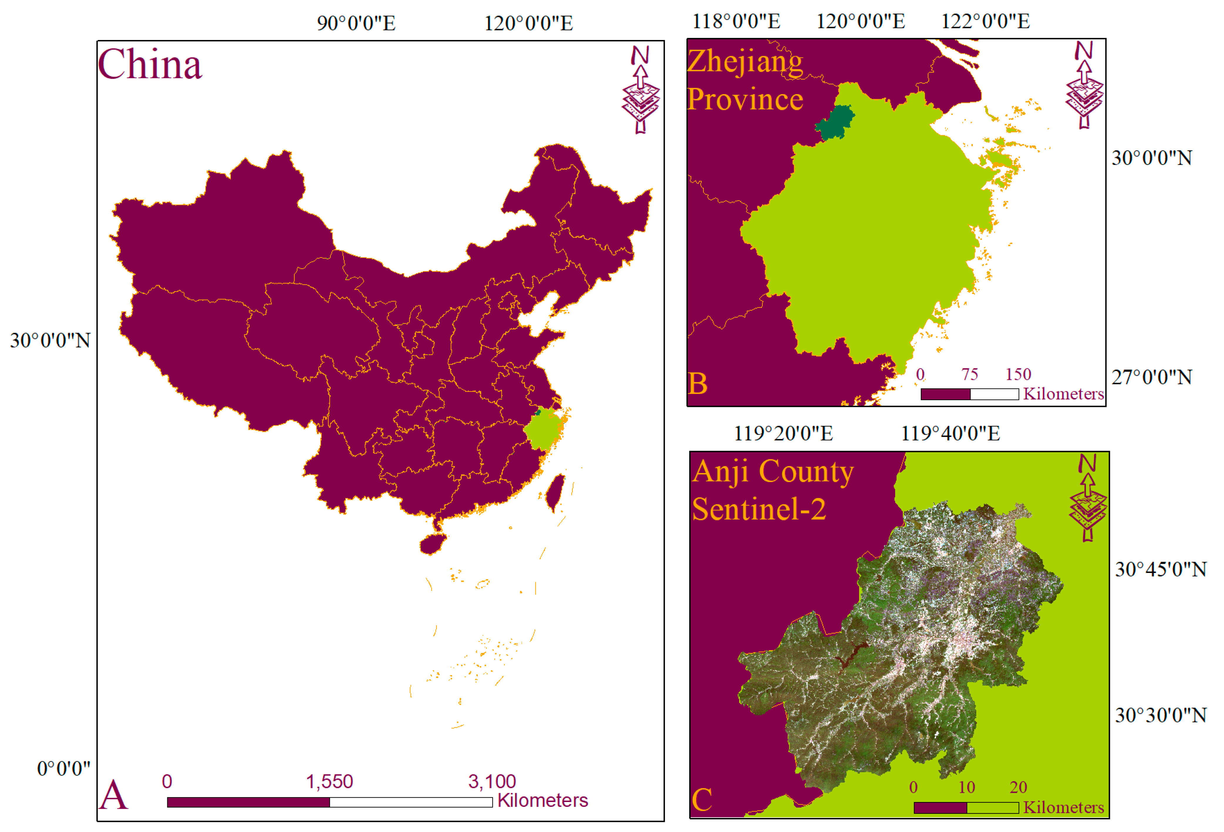
2.1. Study Site
2.2. Field Sampleing
2.3. Satellite Data
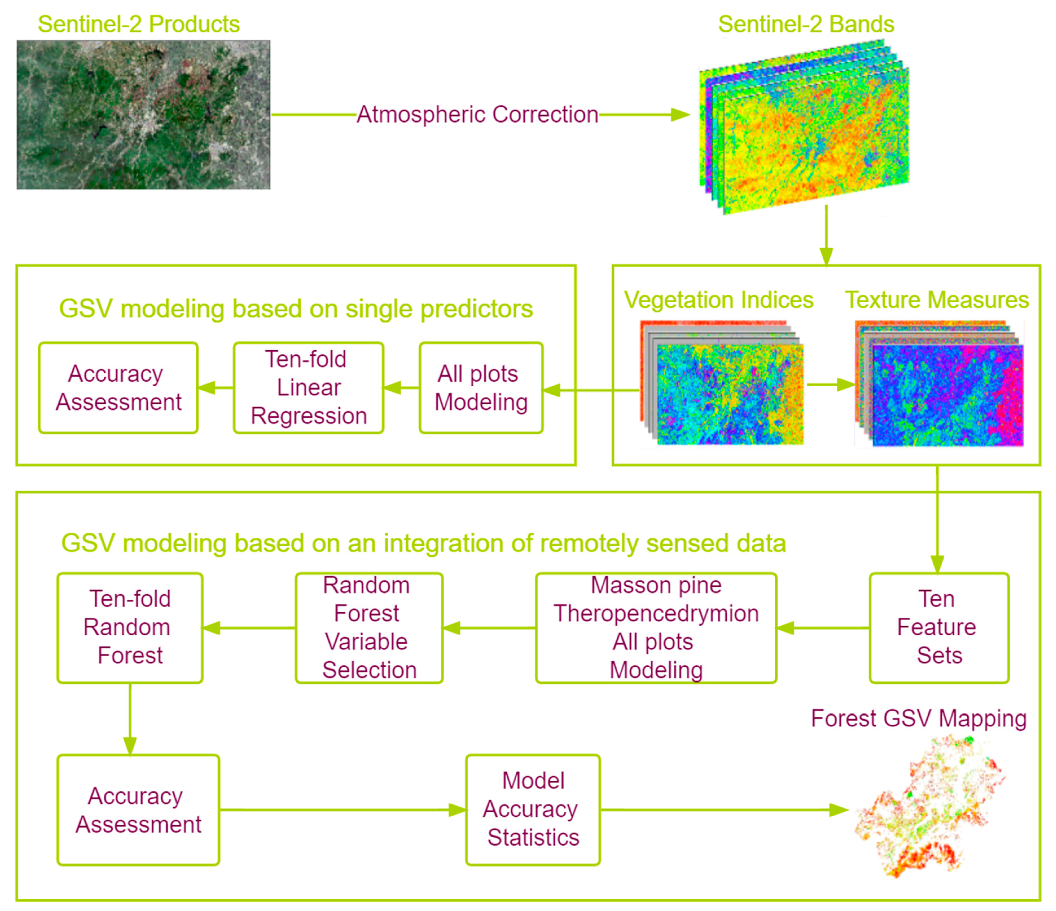
3. Methodology
3.1. Growing Stock Volume Modeling
3.2. Statistical Analyses for Modeling GSV
4. Results
4.1. Relationships between In Situ GSV and Satellite Bands/Vegetation Indices
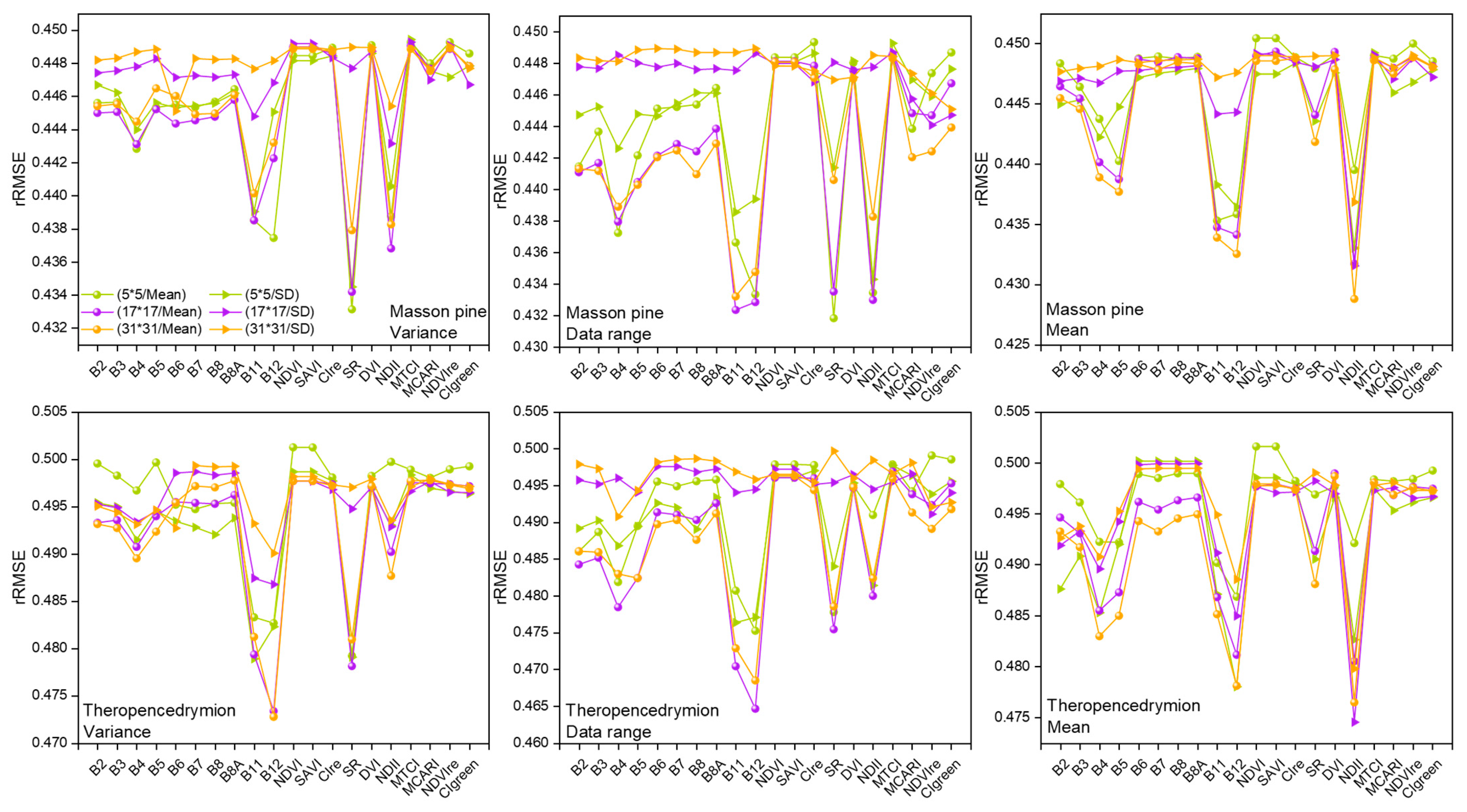
4.2. Relationships between In Situ GSV and Texture Measures
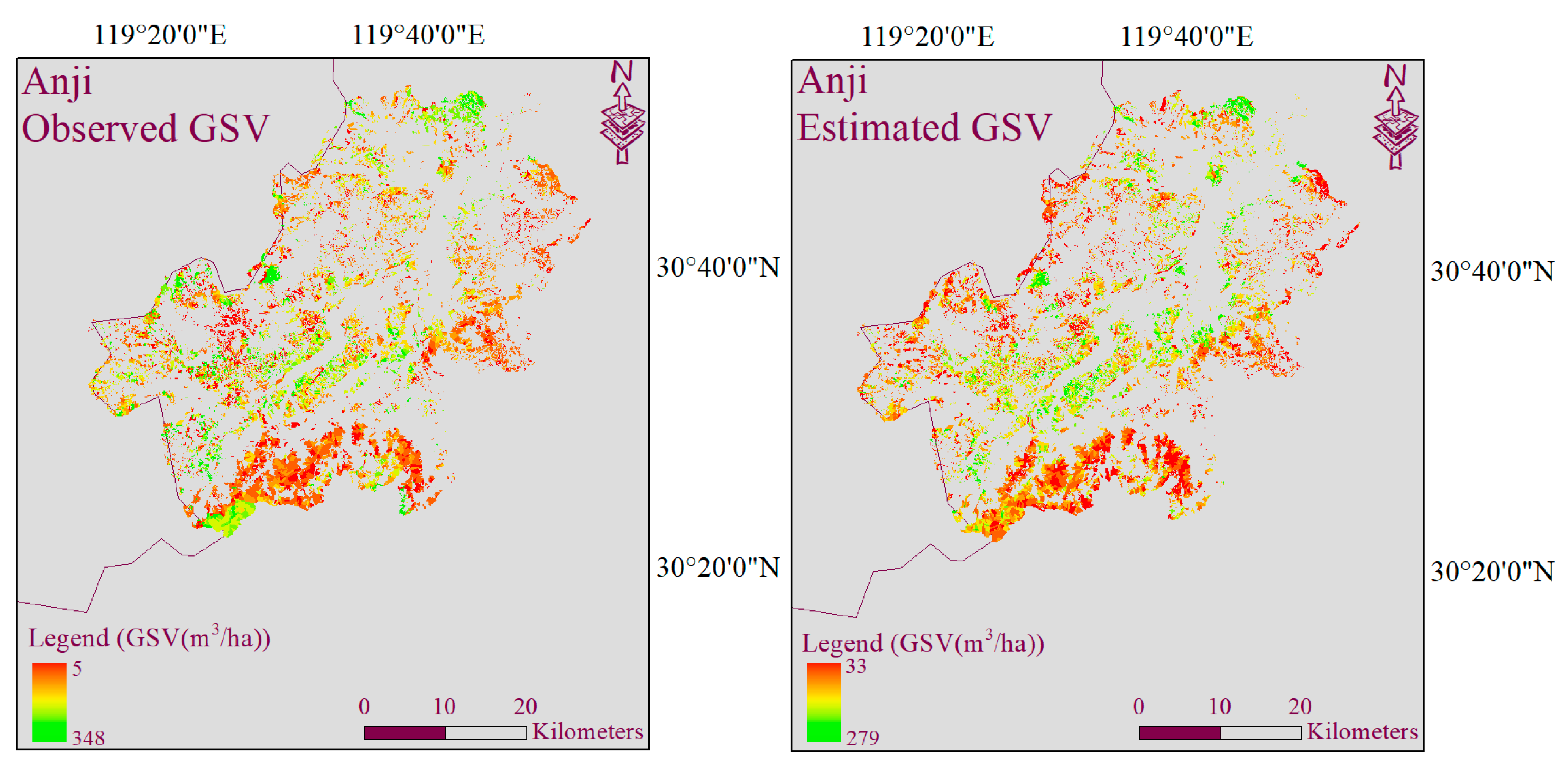
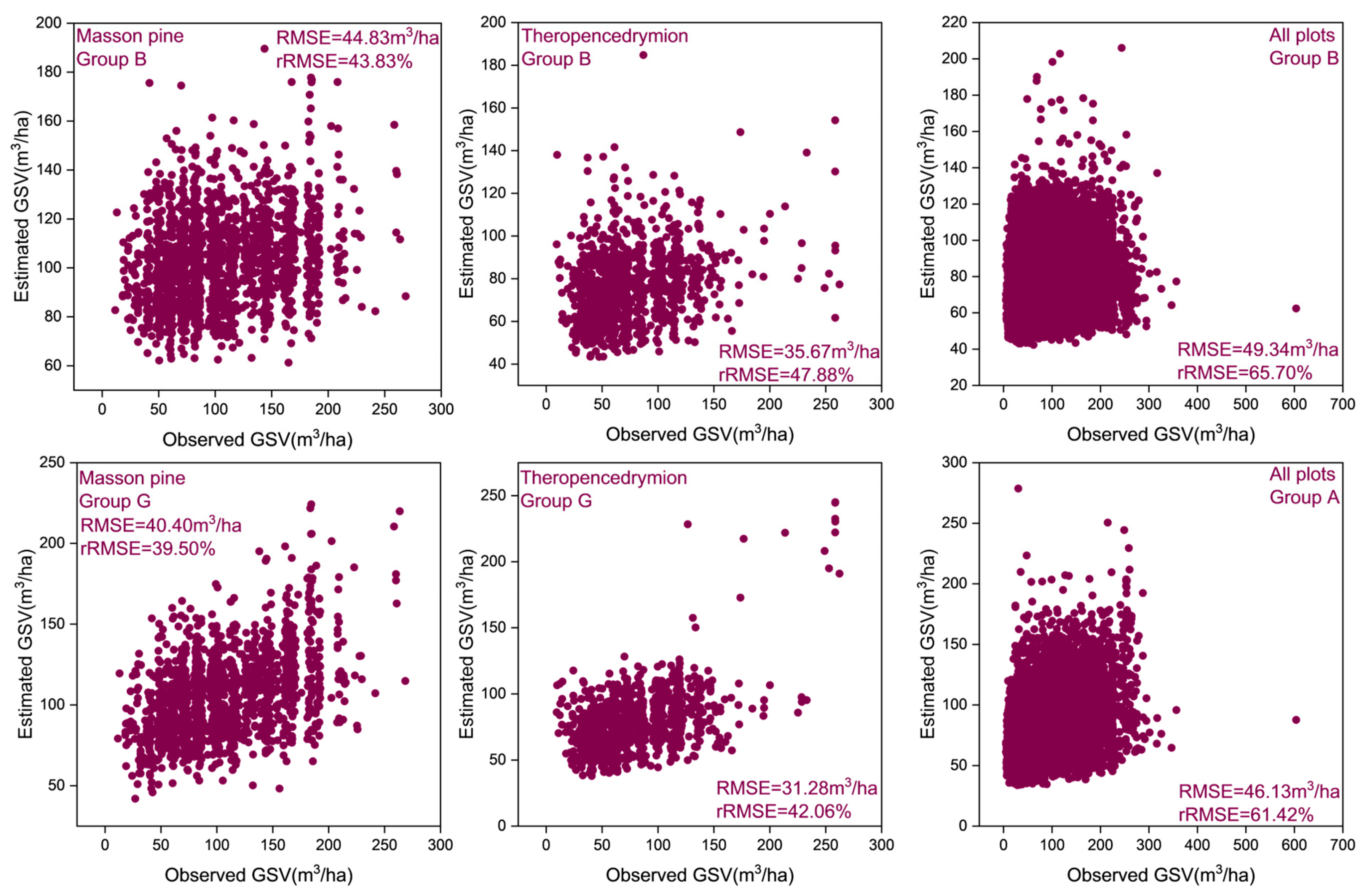
4.3. GSV Modeling and Mapping Using Different Test Setups
5. Discussion
5.1. Bands/VIs for Forest GSV Estimation
5.2. Texture Measures for GSV Estimation
5.3. Multivariate Models for GSV Estimation and Mapping
5.4. Mean Value and Standard Deviation at Plot Level
6. Conclusions
Author Contributions
Funding
Institutional Review Board Statement
Informed Consent Statement
Data Availability Statement
Conflicts of Interest
Appendix A
Appendix B

| Bands/VIs | Variance | Data Range | Mean | RMSE (m3/ha) | r | p | ||||||
|---|---|---|---|---|---|---|---|---|---|---|---|---|
| 5 × 5 | 17 × 17 | 31 × 31 | 5 × 5 | 17 × 17 | 31 × 31 | 5 × 5 | 17 × 17 | 31 × 31 | ||||
| Band 2 | 69.33 | 69.32 | 69.30 | 69.33 | 69.28 | 69.27 | 69.32 | 69.30 | 69.25 | 52.01 | 0.078 | <0.01 |
| Band 3 | 69.32 | 69.29 | 69.26 | 69.32 | 69.26 | 69.26 | 69.30 | 69.21 | 69.15 | 51.93 | 0.110 | <0.01 |
| Band 4 | 69.33 | 69.29 | 69.24 | 69.33 | 69.22 | 69.23 | 69.31 | 69.30 | 69.23 | 51.99 | 0.096 | <0.01 |
| Band 5 | 69.29 | 69.21 | 69.17 | 69.24 | 69.20 | 69.20 | 69.21 | 69.13 | 69.08 | 51.88 | 0.116 | <0.01 |
| Band 6 | 69.23 | 69.32 | 69.23 | 69.29 | 69.30 | 69.24 | 69.30 | 69.32 | 69.33 | 52.00 | −0.060 | <0.01 |
| Band 7 | 69.20 | 69.32 | 69.33 | 69.28 | 69.26 | 69.22 | 69.26 | 69.32 | 69.33 | 51.97 | −0.073 | <0.01 |
| Band 8 | 69.25 | 69.33 | 69.33 | 69.32 | 69.30 | 69.27 | 69.27 | 69.32 | 69.33 | 52.01 | −0.055 | <0.01 |
| Band 8A | 69.24 | 69.33 | 69.33 | 69.30 | 69.27 | 69.24 | 69.29 | 69.33 | 69.33 | 52.00 | 0.095 | <0.01 |
| Band 11 | 69.28 | 69.24 | 69.22 | 69.27 | 69.23 | 69.23 | 69.13 | 69.19 | 69.21 | 51.92 | 0.124 | <0.01 |
| Band 12 | 69.33 | 69.26 | 69.21 | 69.33 | 69.17 | 69.23 | 69.33 | 69.30 | 69.25 | 51.95 | 0.090 | <0.01 |
| NDVI | 69.33 | 69.30 | 69.27 | 69.33 | 69.28 | 69.23 | 69.33 | 69.31 | 69.30 | 52.00 | 0.093 | <0.01 |
| SAVI | 69.33 | 69.30 | 69.27 | 69.33 | 69.28 | 69.23 | 69.33 | 69.31 | 69.30 | 52.00 | 0.093 | <0.01 |
| CIre | 69.33 | 69.32 | 69.31 | 69.33 | 69.32 | 69.28 | 69.33 | 69.32 | 69.32 | 52.04 | 0.080 | <0.01 |
| SR | 68.52 | 69.23 | 69.32 | 69.07 | 69.30 | 69.19 | 68.66 | 69.24 | 69.32 | 51.46 | −0.153 | <0.01 |
| DVI | 69.33 | 69.31 | 69.29 | 69.33 | 69.30 | 69.27 | 69.29 | 69.33 | 69.31 | 52.03 | 0.097 | <0.01 |
| NDII | 69.14 | 69.32 | 69.29 | 69.31 | 69.14 | 68.98 | 69.28 | 69.30 | 69.32 | 51.81 | 0.113 | <0.01 |
| MTCI | 69.33 | 69.33 | 69.32 | 69.33 | 69.33 | 69.32 | 69.33 | 69.33 | 69.32 | 52.06 | 0.084 | <0,01 |
| MCARI | 69.32 | 69.32 | 69.32 | 69.33 | 69.28 | 69.26 | 69.30 | 69.33 | 69.33 | 52.02 | 0.069 | <0.01 |
| NDVIre | 69.33 | 69.30 | 69.27 | 69.33 | 69.29 | 69.24 | 69.33 | 69.32 | 69.30 | 52.00 | 0.107 | <0.01 |
| CIgreen | 69.33 | 69.31 | 69.29 | 69.32 | 69.29 | 69.23 | 69.32 | 69.32 | 69.30 | 52.00 | 0.101 | <0.01 |
| Bands/VIs | Variance | Data Range | Mean | RMSE (m3/ha) | r | p | ||||||
|---|---|---|---|---|---|---|---|---|---|---|---|---|
| 5 × 5 | 17 × 17 | 31 × 31 | 5 × 5 | 17 × 17 | 31 × 31 | 5 × 5 | 17 × 17 | 31 × 31 | ||||
| Band 2 | 69.30 | 69.32 | 69.33 | 69.25 | 69.30 | 69.33 | 69.28 | 69.31 | 69.33 | 52.01 | −0.051 | <0.01 |
| Band 3 | 69.33 | 69.32 | 69.31 | 69.33 | 69.33 | 69.33 | 68.07 | 68.73 | 68.98 | 51.13 | −0.230 | <0.01 |
| Band 4 | 69.31 | 69.33 | 69.32 | 69.21 | 69.31 | 69.29 | 69.24 | 69.27 | 69.29 | 51.98 | −0.064 | <0.01 |
| Band 5 | 69.30 | 69.26 | 69.23 | 69.30 | 69.31 | 69.29 | 67.09 | 67.97 | 68.41 | 50.38 | −0.304 | <0.01 |
| Band 6 | 69.13 | 69.17 | 69.16 | 69.10 | 69.16 | 69.28 | 65.94 | 67.49 | 68.12 | 49.52 | −0.355 | <0.01 |
| Band 7 | 69.02 | 69.10 | 69.20 | 68.95 | 69.10 | 69.27 | 66.19 | 67.65 | 68.23 | 49.71 | −0.347 | <0.01 |
| Band 8 | 69.14 | 69.16 | 69.24 | 69.15 | 69.20 | 69.29 | 65.99 | 67.52 | 68.12 | 49.56 | −0.354 | <0.01 |
| Band 8A | 69.11 | 69.18 | 69.26 | 69.06 | 69.18 | 69.30 | 66.06 | 67.50 | 68.11 | 49.62 | −0.353 | <0.01 |
| Band 11 | 69.30 | 69.31 | 69.30 | 69.26 | 69.31 | 69.31 | 66.08 | 67.21 | 67.72 | 49.63 | −0.335 | <0.01 |
| Band 12 | 69.31 | 69.32 | 69.33 | 69.28 | 69.31 | 69.33 | 68.08 | 68.48 | 68.67 | 51.13 | −0.221 | <0.01 |
| NDVI | 69.33 | 69.32 | 69.31 | 69.33 | 69.33 | 69.31 | 69.28 | 69.33 | 69.33 | 52.04 | −0.137 | <0.01 |
| SAVI | 69.33 | 69.32 | 69.31 | 69.33 | 69.33 | 69.31 | 69.28 | 69.33 | 69.33 | 52.04 | −0.137 | <0.01 |
| CIre | 69.32 | 69.32 | 69.33 | 69.32 | 69.33 | 69.33 | 69.32 | 69.32 | 69.33 | 52.07 | −0.102 | <0.01 |
| SR | 68.27 | 68.55 | 68.84 | 68.15 | 68.77 | 69.10 | 68.58 | 69.05 | 69.16 | 51.18 | −0.178 | <0.01 |
| DVI | 69.33 | 69.33 | 69.32 | 69.28 | 69.33 | 69.32 | 66.96 | 68.95 | 69.19 | 50.29 | −0.315 | <0.01 |
| NDII | 69.30 | 69.29 | 69.29 | 69.24 | 69.31 | 69.32 | 69.27 | 69.16 | 69.14 | 51.93 | −0.021 | 0.011 |
| MTCI | 69.33 | 69.33 | 69.33 | 69.33 | 69.33 | 69.33 | 69.33 | 69.33 | 69.33 | 52.07 | 0.026 | 0.002 |
| MCARI | 69.33 | 69.33 | 69.33 | 69.29 | 69.33 | 69.33 | 67.49 | 68.76 | 69.01 | 50.69 | −0.282 | <0.01 |
| NDVIre | 69.33 | 69.33 | 69.32 | 69.32 | 69.33 | 69.32 | 69.30 | 69.33 | 69.33 | 52.05 | −0.111 | <0.01 |
| CIgreen | 69.33 | 69.33 | 69.33 | 69.33 | 69.32 | 69.31 | 69.33 | 69.33 | 69.33 | 52.06 | 0.012 | 0.148 |
Appendix C
| Experiment | Tree Species | ||
|---|---|---|---|
| Masson Pine | Theropencedrymion | All Plots | |
| A | S2_B11M (12.24), | S2_B12M (11.06), | S2_B8M (14.02), |
| S2_B2M (10.82), | S2_B2M (10.21), | S2_B11M (9.16), | |
| MTCIM (8.03), | MTCIM (9.44), | MTCIM (7.35), | |
| S2_B3M (6.13) | S2_B11M (8.24) | MCARIM (7.33) | |
| B | S2_B12SD (8.89), | S2_B12SD (14.84), | SRSD (10.4), |
| SRSD (8.16), | CIgreenSD (7.55), | S2_B11SD (8.17), | |
| NDIISD (7.47), | SRSD (7.04), | MCARISD (7.43), | |
| MCARISD (6.92) | MTCISD (6.72) | CIgreenSD (6.1) | |
| C | B11_RA17M (4.46), | B12_VA31M (7.62), | S2_B8M (12.13), |
| MTCIM (4.74), | MTCIM (6.91), | MCARIM (3.58), | |
| MCARIM (3.65), | B12_RA31M (3.22), | S2_B11M (3.37), | |
| B12_VA31M (3.07) | B12_VA17M (3.1) | MTCIM (3.37) | |
| D | S2_B11M (5.04), | MTCIM (6.05), | S2_B8M (3.65), |
| S2_B2M (3.76), | B11_VA5SD (4.98), | S2_B11M (5.26), | |
| MTCIM (3.69), | S2_B11M (3.38), | MTCIM (3.18), | |
| MCARIM (2.94) | S2_B2M (3.05) | MCARIM (3.65) | |
| E | B11_RA17M (4.46), | B12_VA31M (7.54), | B8_ME5M (9.53), |
| B2_ME5M (3.06), | B12_VA17M (3.61), | B11_ME5M (5.58), | |
| B12_VA31M (2.8), | B12_RA31M (3.1), | B5_ME31M (2.33), | |
| B11_ME31M (2.29) | B11_VA31M (2.62) | B6_ME5M (1.97) | |
| F | B11_VA5SD (3.41), | B11_VA5SD (4.6), | SRSD (6.32), |
| SRSD (3.2), | B11_RA5SD (3.02), | S2_B11SD (3.57), | |
| B4_ME5SD (2.81), | B12_VA5SD (2.83), | MCARISD (3.12), | |
| MCARISD (2.34) | S2_B12SD (2.74) | CIgreenSD (2.29) | |
| G | NDII_ME31M (12.22), | MTCI_ME31M (4.42), | S2_B8M (12.14), |
| MCARI_ME31M (3.2), | NDII_ME31M (3.51), | S2_B11M (4.48), | |
| S2_B4M (3.16), | SR_RA31M (3.42), | MTCIM (3.47), | |
| MTCIM (2.69) | NDII_VA31M (3.04) | MCARIM (2.49) | |
| H | NDII_ME17SD (6.58), | NDII_ME17SD (6.47), | S2_B8M (12.01), |
| NDII_ME5SD (4.16), | NDII_ME31SD (6.4), | S2_B11M (4.68), | |
| MCARIM (3.38), | MTCIM (5.87), | MCARIM (3.68), | |
| MTCIM (2.8) | S2_B2M (3.32) | MTCIM (3.01) | |
| I | NDII_ME31M (11.94), | MTCI_ME31M (4.6), | DVI_ME5M (10.16), |
| MTCI_ME31M (3.83), | SR_RA31M (4.45), | MCARI_ME5M (4), | |
| SR_RA31M (2.93), | NDVI_VA31M (3.23), | MTCI_ME5M (2.12), | |
| MTCI_ME5M (2.48) | NDVIre_VA31M (3.3) | SR_VA5M (2.11) | |
| J | NDII_ME17SD (6.74), | NDII_ME31SD (8.01), | SRSD (5.34), |
| NDII_ME5SD (3.68), | NDII_ME17SD (4.5), | S2_B11SD (4.06), | |
| S2_B4SD (2.5), | NDII_ME5SD (2.17), | MCARISD (2.38), | |
| NDII_ME31SD (2.28) | S2_B8SD (1.9) | MCARI_VA5SD (1.91) | |
References
- Santoro, M.; Beer, C.; Cartus, O.; Schmullius, C.; Shvidenko, A.; McCallum, I.; Wegmüller, U.; Wiesmann, A. Retrieval of growing stock volume in boreal forest using hyper-temporal series of Envisat ASAR ScanSAR backscatter measurements. Remote Sens. Environ. 2011, 115, 490–507. [Google Scholar] [CrossRef]
- Seidl, R.; Schelhaas, M.-J.; Rammer, W.; Verkerk, P.J. Increasing forest disturbances in Europe and their impact on carbon storage. Nat. Clim. Chang. 2014, 4, 806–810. [Google Scholar] [CrossRef] [PubMed]
- Ozdemir, I.; Karnieli, A. Predicting forest structural parameters using the image texture derived from WorldView-2 multispectral imagery in a dryland forest, Israel. Int. J. Appl. Earth Obs. Geoinf. 2011, 13, 701–710. [Google Scholar] [CrossRef]
- Puliti, S.; Saarela, S.; Gobakken, T.; Ståhl, G.; Næsset, E. Combining UAV and Sentinel-2 auxiliary data for forest growing stock volume estimation through hierarchical model-based inference. Remote Sens. Environ. 2018, 204, 485–497. [Google Scholar] [CrossRef]
- Sánchez-Ruiz, S.; Moreno-Martínez, Á.; Izquierdo-Verdiguier, E.; Chiesi, M.; Maselli, F.; Gilabert, M.A. Growing stock volume from multi-temporal landsat imagery through google earth engine. Int. J. Appl. Earth Obs. Geoinf. 2019, 83, 101913. [Google Scholar] [CrossRef]
- Astola, H.; Häme, T.; Sirro, L.; Molinier, M.; Kilpi, J. Comparison of Sentinel-2 and Landsat 8 imagery for forest variable prediction in boreal region. Remote Sens. Environ. 2019, 223, 257–273. [Google Scholar] [CrossRef]
- Drusch, M.; Del Bello, U.; Carlier, S.; Colin, O.; Fernandez, V.; Gascon, F.; Hoersch, B.; Isola, C.; Laberinti, P.; Martimort, P.; et al. Sentinel-2: ESA’s Optical High-Resolution Mission for GMES Operational Services. Remote Sens. Environ. 2012, 120, 25–36. [Google Scholar] [CrossRef]
- Chrysafis, I.; Mallinis, G.; Siachalou, S.; Patias, P. Assessing the relationships between growing stock volume and Sentinel-2 imagery in a Mediterranean forest ecosystem. Remote Sens. Lett. 2017, 8, 508–517. [Google Scholar] [CrossRef]
- Mura, M.; Bottalico, F.; Giannetti, F.; Bertani, R.; Giannini, R.; Mancini, M.; Orlandini, S.; Travaglini, D.; Chirici, G. Exploiting the capabilities of the Sentinel-2 multi spectral instrument for predicting growing stock volume in forest ecosystems. Int. J. Appl. Earth Obs. Geoinf. 2018, 66, 126–134. [Google Scholar] [CrossRef]
- Lu, D.; Chen, Q.; Wang, G.; Liu, L.; Li, G.; Moran, E. A survey of remote sensing-based aboveground biomass estimation methods in forest ecosystems. Int. J. Digit. Earth 2016, 9, 63–105. [Google Scholar] [CrossRef]
- Zeng, Y.; Hao, D.; Huete, A.; Dechant, B.; Berry, J.; Chen, J.M.; Joiner, J.; Frankenberg, C.; Ben Bond-Lamberty, B.; Ryu, Y.; et al. Optical vegetation indices for monitoring terrestrial ecosystems globally. Nat. Rev. Earth Environ. 2022, 3, 477–493. [Google Scholar] [CrossRef]
- Kobayashi, H.; Dye, D.G. Atmospheric conditions for monitoring the long-term vegetation dynamics in the Amazon using normalized difference vegetation index. Remote Sens. Environ. 2005, 97, 519–525. [Google Scholar] [CrossRef]
- Chen, S.; Useya, J.; Mugiyo, H. Decision-level fusion of Sentinel-1 SAR and Landsat 8 OLI texture features for crop discrimination and classification: Case of Masvingo, Zimbabwe. Heliyon 2020, 6, e05358. [Google Scholar] [CrossRef] [PubMed]
- Lu, D.; Batistella, M. Exploring TM Image Texture and its Relationships with Biomass Estimation in Rondônia, Brazilian Amazon. Acta Amaz. 2005, 35, 249–257. [Google Scholar] [CrossRef]
- Chrysafis, I.; Mallinis, G.; Tsakiri, M.; Patias, P. Evaluation of single-date and multi-seasonal spatial and spectral information of Sentinel-2 imagery to assess growing stock volume of a Mediterranean forest. Int. J. Appl. Earth Obs. Geoinf. 2019, 77, 1–14. [Google Scholar] [CrossRef]
- Li, X.; Liu, Z.; Lin, H.; Wang, G.; Sun, H.; Long, J.; Zhang, M. Estimating the Growing Stem Volume of Chinese Pine and Larch Plantations based on Fused Optical Data Using an Improved Variable Screening Method and Stacking Algorithm. Remote Sens. 2020, 12, 871. [Google Scholar] [CrossRef]
- Wood, E.M.; Pidgeon, A.M.; Radeloff, V.C.; Keuler, N.S. Image Texture Predicts Avian Density and Species Richness. PLoS ONE 2013, 8, e63211. [Google Scholar] [CrossRef]
- Ozdemir, I.; Mert, A.; Ozkan, U.Y.; Aksan, S.; Unal, Y. Predicting bird species richness and micro-habitat diversity using satellite data. For. Ecol. Manag. 2018, 424, 483–493. [Google Scholar] [CrossRef]
- St-Louis, V.; Pidgeon, A.M.; Radeloff, V.C.; Hawbaker, T.J.; Clayton, M.K. High-resolution image texture as a predictor of bird species richness. Remote Sens. Environ. 2006, 105, 299–312. [Google Scholar] [CrossRef]
- Nie, W.; Shi, Y.; Siaw, M.J.; Yang, F.; Wu, R.; Wu, X.; Zheng, X.; Bao, Z. Constructing and optimizing ecological network at county and town Scale: The case of Anji County, China. Ecol. Indic. 2021, 132, 108294. [Google Scholar] [CrossRef]
- Zhang, J.; Ge, Y.; Chang, J.; Jiang, B.; Jiang, H.; Peng, C.; Zhu, J.; Yuan, W.; Qi, L.; Yu, S. Carbon storage by ecological service forests in Zhejiang Province, subtropical China. For. Ecol. Manag. 2007, 245, 64–75. [Google Scholar] [CrossRef]
- JRouse, W.; Haas, R.H.; Schell, J.A.; Deering, W.D. Monitoring vegetation systems in the Great Plains with ERTS. Third ERTS Symp. 1973, 351, 309–317. [Google Scholar]
- Huete, A. A soil-adjusted vegetation index (SAVI). Remote Sens. Environ. 1988, 25, 295–309. [Google Scholar] [CrossRef]
- Gitelson, A.A.; Gritz, Y.; Merzlyak, M.N. Relationships between leaf chlorophyll content and spectral reflectance and algorithms for non-destructive chlorophyll assessment in higher plant leaves. J. Plant Physiol. 2003, 160, 271–282. [Google Scholar] [CrossRef]
- Jordan, C.F. Derivation of Leaf-Area Index from Quality of Light on the Forest Floor. Ecology 1969, 50, 663–666. [Google Scholar] [CrossRef]
- Hardisky, M.A.; Daiber, F.C.; Roman, C.T.; Klemas, V. Remote sensing of biomass and annual net aerial primary productivity of a salt marsh. Remote Sens. Environ. 1984, 16, 91–106. [Google Scholar] [CrossRef]
- Dash, J.; Curran, P.J. The MERIS terrestrial chlorophyll index. Int. J. Remote Sens. 2004, 25, 5403–5413. [Google Scholar] [CrossRef]
- Daughtry, C. Estimating Corn Leaf Chlorophyll Concentration from Leaf and Canopy Reflectance. Remote Sens. Environ. 2000, 74, 229–239. [Google Scholar] [CrossRef]
- Gitelson, A.; Merzlyak, M.N. Spectral Reflectance Changes Associated with Autumn Senescence of Aesculus hippocastanum L. and Acer platanoides L. Leaves. Spectral Features and Relation to Chlorophyll Estimation. J. Plant Physiol. 1994, 143, 286–292. [Google Scholar] [CrossRef]
- Breiman, L.E.O. Random Forests. Mach. Learn. 2001, 45, 5–32. [Google Scholar] [CrossRef]
- Mutanga, O.; Adam, E.; Cho, M.A. High density biomass estimation for wetland vegetation using WorldView-2 imagery and random forest regression algorithm. Int. J. Appl. Earth Obs. Geoinf. 2012, 18, 399–406. [Google Scholar] [CrossRef]
- Belgiu, M.; Dra, L. Random forest in remote sensing: A review of applications and future directions. ISPRS J. Photogramm. Remote Sens. 2016, 114, 24–31. [Google Scholar] [CrossRef]
- Wang, J.; Xiao, X.; Bajgain, R.; Starks, P.; Steiner, J.; Doughty, R.B.; Chang, Q. Estimating leaf area index and aboveground biomass of grazing pastures using Sentinel-1, Sentinel-2 and Landsat images. ISPRS J. Photogramm. Remote Sens. 2019, 154, 189–201. [Google Scholar] [CrossRef]
- Ndikumana, E.; Minh, D.H.T.; Nguyen, H.T.D.; Baghdadi, N.; Courault, D.; Hossard, L.; El Moussawi, I. Estimation of rice height and biomass using multitemporal SAR Sentinel-1 for Camargue, Southern France. Remote Sens. 2018, 10, 1394. [Google Scholar] [CrossRef]
- Szantoi, Z.; Escobedo, F.; Abd-Elrahman, A.; Smith, S.; Pearlstine, L. Analyzing fine-scale wetland composition using high resolution imagery and texture features. Int. J. Appl. Earth Obs. Geoinf. 2013, 23, 204–212. [Google Scholar] [CrossRef]
- Camps-Valls, G.; Campos-Taberner, M.; Moreno-Martínez, A.; Walther, S.; Duveiller, G.; Cescatti, A.; Mahecha, M.D.; Muñoz-Marí, J.; García-Haro, F.J.; Guanter, L.; et al. A unified vegetation index for quantifying the terrestrial biosphere. Sci. Adv. 2021, 7, eabc7447. [Google Scholar] [CrossRef]
- Wood, E.M.; Pidgeon, A.M.; Radeloff, V.C.; Keuler, N.S. Image texture as a remotely sensed measure of vegetation structure. Remote Sens. Environ. 2012, 121, 516–526. [Google Scholar] [CrossRef]
- Korhonen, L.; Hadi; Packalen, P.; Rautiainen, M. Comparison of Sentinel-2 and Landsat 8 in the estimation of boreal forest canopy cover and leaf area index. Remote Sens. Environ. 2017, 195, 259–274. [Google Scholar] [CrossRef]
- Forkuor, G.; Zoungrana, J.-B.B.; Dimobe, K.; Ouattara, B.; Vadrevu, K.P.; Tondoh, J.E. Above-ground biomass mapping in West African dryland forest using Sentinel-1 and 2 datasets—A case study. Remote Sens. Environ. 2020, 236, 111496. [Google Scholar] [CrossRef]
- Li, X.; Lin, H.; Long, J.; Xu, X. Mapping the Growing Stem Volume of the Coniferous Plantations in North China Using Multispectral Data from Integrated GF-2 and Sentinel-2 Images and an Optimized Feature Variable Selection Method. Remote Sens. 2021, 13, 2740. [Google Scholar] [CrossRef]
- Houghton, R.A.; Butman, D.; Bunn, A.G.; Krankina, O.N.; Schlesinger, P.; Stone, T.A. Mapping Russian forest biomass with data from satellites and forest inventories. Environ. Res. Lett. 2007, 2, 045032. [Google Scholar] [CrossRef]
- Kankare, V.; Vastaranta, M.; Holopainen, M.; Räty, M.; Yu, X.; Hyyppä, J.; Hyyppä, H.; Alho, P.; Viitala, R. Retrieval of Forest Aboveground Biomass and Stem Volume with Airborne Scanning LiDAR. Remote Sens. 2013, 5, 2257–2274. [Google Scholar] [CrossRef]
- Zhou, R.; Wu, D.; Fang, L.; Xu, A.; Lou, X. A Levenberg–Marquardt Backpropagation Neural Network for Predicting Forest Growing Stock Based on the Least-Squares Equation Fitting Parameters. Forests 2018, 9, 757. [Google Scholar] [CrossRef]
- Lu, D.; Mausel, P.; Brondı, E.; Moran, E. Relationships between forest stand parameters and Landsat TM spectral responses in the Brazilian Amazon Basin. For. Ecol. Manag. 2004, 198, 149–167. [Google Scholar] [CrossRef]
- Zhao, Q.; Yu, S.; Zhao, F.; Tian, L.; Zhao, Z. Comparison of machine learning algorithms for forest parameter estimations and application for forest quality assessments. For. Ecol. Manag. 2019, 434, 224–234. [Google Scholar] [CrossRef]
- Yu, X.; Ge, H.; Lu, D.; Zhang, M.; Lai, Z.; Yao, R. Comparative study on variable selection approaches in establishment of remote sensing model for forest biomass estimation. Remote Sens. 2019, 11, 1437. [Google Scholar] [CrossRef]
- Macedo, F.L.; Sousa, A.M.O.; Gonçalves, A.C.; da Silva, J.R.M.; Mesquita, P.A.; Rodrigues, R.A.F. Above-ground biomass estimation for Quercus rotundifolia using vegetation indices derived from high spatial resolution satellite images. Eur. J. Remote Sens. 2018, 51, 932–944. [Google Scholar] [CrossRef]
| Forest Variable | Masson Pine | Theropencedrymion | All Plots | |||
|---|---|---|---|---|---|---|
| Mean | Stdev | Mean | Stdev | Mean | Stdev | |
| Number of stems (stems/ha) | 847 | 316 | 1150 | 589 | 1275 | 948 |
| Number of plots | 1808 | 1214 | 14,271 | |||
| Age (year) | 35.39 | 7.39 | 30.53 | 9.48 | 29.09 | 9.13 |
| Canopy Cover (%) | 72.01 | 12.25 | 74.02 | 11.31 | 73.29 | 10.76 |
| GSV (m3/ha) | 102.28 | 45.93 | 74.55 | 37.34 | 75.11 | 52.08 |
| Bands/Vegetation Indices | Bands/Indices | Description |
|---|---|---|
| Bands | Band 2 | Blue, 490 nm, 10 m |
| Band 3 | Green, 560 nm,10 m | |
| Band 4 | Red, 665 nm, 10 m | |
| Band 5 | Red edge, 705 nm, 20 m | |
| Band 6 | Red edge, 749 nm, 20 m | |
| Band 7 | Red edge, 783 nm, 20 m | |
| Band 8 | Near infrared, 842 nm, 10 m | |
| Band 8A | Near infrared narrow, 865 nm, 20 m | |
| Band 11 | Shortwave infrared 1, 1610 nm, 20 m | |
| Band 12 | Shortwave infrared 2, 2190 nm, 20 m | |
| Vegetation indices | NDVI | [22] |
| SAVI | [23] | |
| CIgreen | [24] | |
| SR | [25] | |
| DVI | B8 − B4 [25] | |
| NDII | [26] | |
| Red-edge vegetation indices | MTCI | [27] |
| MCARI | [28] | |
| NDVIre | [29] | |
| CIre | [24] |
| Texture Metrics | Formula |
|---|---|
| Mean | |
| Where represents the gray tone values of pixel k, N represents the number of gray tone values | |
| Data range | |
| Where represents | |
| Variance |
| Experiment | Description |
|---|---|
| A: S2M | All bands and vegetation indices based on MV |
| B: S2SD | All bands and vegetation indices based on STD |
| C: S2M + Bands_TMM | Synergizing all S2 predictors based on MV and texture measures derived from bands based on MV |
| D: S2M + Bands_TMSD | Synergizing all S2 predictors based on MV and texture measures derived from bands based on STD |
| E: S2SD + Bands_TMM | Synergizing all S2 predictors based on STD and texture measures derived from bands based on MV |
| F: S2SD + Bands_TMSD | Synergizing all S2 predictors based on STD and texture measures derived from bands based on STD |
| G: S2M + VI_TMM | Synergizing all S2 predictors based on MV and texture measures derived from vegetation indices based on MV |
| H: S2M + VI_TMSD | Synergizing all S2 predictors based on MV and texture measures derived from vegetation indices based on STD |
| I: S2SD + VI_TMM | Synergizing all S2 predictors based on STD and texture measures derived from vegetation indices based on MV |
| J: S2SD + VI_TMSD | Synergizing all S2 predictors based on STD and texture measures derived from vegetation indices based on STD |
| Predicted Variables | Bands/ Indices | Standard Deviation | Mean | ||||||
|---|---|---|---|---|---|---|---|---|---|
| r | R2 | RMSE (m3/ha) | rRMSE (%) | r | R2 | RMSE (m3/ha) | rRMSE (%) | ||
| Bands | Band 2 | −0.043 ** | 0.0003 | 52.04 | 69.29 | −0.043 ** | 0.0007 | 52.03 | 69.28 |
| Band 3 | 0.032 ** | −0.0006 | 52.07 | 69.32 | −0.253 ** | 0.0407 | 50.98 | 67.88 | |
| Band 4 | −0.057 ** | 0.0007 | 52.03 | 69.28 | −0.055 ** | 0.0014 | 52.01 | 69.25 | |
| Band 5 | 0.078 ** | 0.0015 | 52.01 | 69.25 | −0.319 ** | 0.0678 | 50.26 | 66.91 | |
| Band 6 | −0.037 ** | 0.0003 | 52.04 | 69.29 | −0.375 ** | 0.1070 | 49.19 | 65.46 | |
| Band 7 | −0.062 ** | 0.0021 | 51.99 | 69.23 | −0.365 ** | 0.0995 | 49.39 | 65.76 | |
| Band 8 | −0.040 ** | 0.0003 | 52.04 | 69.29 | −0.375 ** | 0.1080 | 49.16 | 65.45 | |
| Band 8A | −0.049 ** | 0.0011 | 52.02 | 69.27 | −0.369 ** | 0.1024 | 49.31 | 65.65 | |
| Band 11 | 0.135 ** | 0.0062 | 51.89 | 69.09 | −0.351 ** | 0.0985 | 49.42 | 65.80 | |
| Band 12 | 0.010 | −0.0005 | 52.06 | 69.32 | −0.236 ** | 0.0374 | 51.07 | 67.99 | |
| Vegetation | NDVI | −0.040 ** | −0.0014 | 52.09 | 69.35 | −0.176 ** | 0.0085 | 51.83 | 69.01 |
| Indices | SAVI | −0.040 ** | −0.0014 | 52.09 | 69.35 | −0.176 ** | 0.0085 | 51.83 | 69.01 |
| CIre | −0.084 ** | −0.0006 | 52.07 | 69.32 | −0.153 ** | −0.0006 | 52.07 | 69.33 | |
| SR | −0.187 ** | 0.0281 | 51.31 | 68.32 | −0.203 ** | 0.0283 | 51.31 | 68.31 | |
| DVI | −0.107 ** | 0.0005 | 52.04 | 69.29 | −0.343 ** | 0.0876 | 49.72 | 66.19 | |
| NDII | −0.028 ** | −0.0007 | 52.07 | 69.33 | −0.092 ** | −0.0007 | 52.07 | 69.33 | |
| MTCI | −0.016 | −0.0010 | 52.08 | 69.34 | −0.047 ** | −0.0005 | 52.06 | 69.32 | |
| MCARI | −0.047 ** | −0.0002 | 52.06 | 69.31 | −0.316 ** | 0.0761 | 50.03 | 66.61 | |
| NDVIre | −0.020 * | −0.0005 | 52.06 | 69.32 | −0.143 ** | 0.0027 | 51.98 | 69.21 | |
| CIgreen | −0.125 ** | −0.0005 | 52.06 | 69.32 | −0.190 ** | −0.0008 | 52.07 | 69.33 | |
| Predicted Variables | Bands/ Indices | Masson Pine | Theropencedrymion | ||||||
|---|---|---|---|---|---|---|---|---|---|
| Standard Deviation | rRMSESD (%) | Mean | rRMSEM (%) | Standard Deviation | rRMSESD (%) | Mean | rRMSEM (%) | ||
| Bands | Band 2 | −0.166 ** | 44.52 | 0.064 ** | 44.90 | −0.233 ** | 48.86 | 0.042 | 49.87 |
| Band 3 | −0.135 ** | 44.53 | −0.036 | 44.72 | −0.181 ** | 49.14 | −0.029 | 49.73 | |
| Band 4 | −0.205 ** | 44.24 | −0.043 | 44.63 | −0.269 ** | 48.67 | −0.069 * | 49.51 | |
| Band 5 | −0.167 ** | 44.39 | −0.156 ** | 44.13 | −0.204 ** | 49.13 | −0.158 ** | 49.20 | |
| Band 6 | −0.094 ** | 44.70 | −0.060 * | 44.85 | −0.070 * | 50.00 | −0.035 | 49.83 | |
| Band 7 | −0.085 ** | 44.74 | −0.053 * | 44.87 | −0.080 ** | 50.00 | −0.029 | 49.81 | |
| Band 8 | −0.079 ** | 44.76 | −0.075 ** | 44.82 | −0.057 * | 50.00 | −0.047 | 49.85 | |
| Band 8A | −0.074 ** | 44.77 | −0.059 * | 44.86 | −0.067 * | 50.00 | −0.040 | 49.84 | |
| Band 11 | −0.229 ** | 43.69 | −0.231 ** | 43.61 | −0.258 ** | 48.59 | −0.263 ** | 48.97 | |
| Band 12 | −0.259 ** | 43.55 | −0.205 ** | 43.71 | −0.317 ** | 47.79 | −0.255 ** | 48.84 | |
| Vegetation | NDVI | −0.214 ** | 48.17 | 0.010 | 44.83 | −0.263 ** | 50.90 | 0.046 | 49.62 |
| Indices | SAVI | −0.214 ** | 48.17 | 0.010 | 44.83 | −0.263 ** | 50.90 | 0.046 | 49.62 |
| CIre | −0.108 ** | 44.89 | 0.062 ** | 44.94 | −0.141 ** | 18.80 | 0.095 * | 118.83 | |
| SR | −0.218 ** | 43.96 | −0.022 | 44.90 | −0.290 ** | 48.70 | 0.005 | 49.84 | |
| DVI | −0.142 ** | 46.22 | −0.052 * | 44.88 | −0.142 ** | 49.63 | −0.013 | 49.79 | |
| NDII | −0.231 ** | 44.25 | −0.043 | 44.66 | −0.275 ** | 49.21 | −0.006 | 49.82 | |
| MTCI | −0.137 ** | 44.95 | 0.130 ** | 44.90 | −0.193 ** | 49.81 | 0.161 ** | 49.83 | |
| MCARI | −0.157 ** | 44.62 | −0.111 ** | 44.65 | −0.203 ** | 49.53 | −0.052 | 49.87 | |
| NDVIre | −0.198 ** | 44.86 | 0.074 ** | 44.70 | −0.247 ** | 49.73 | 0.098 ** | 49.29 | |
| CIgreen | −0.168 ** | 44.88 | −0.046 | 44.99 | −0.220 ** | 49.81 | 0.024 | 49.82 | |
| Experiment | Survey Plots | |||||
|---|---|---|---|---|---|---|
| Masson Pine | Theropencedrymion | All Plots | ||||
| RMSE (m3/ha) | rRMSE (%) | RMSE (m3/ha) | rRMSE (%) | RMSE (m3/ha) | rRMSE (%) | |
| A | 42.63 | 41.71 | 39.90 | 45.54 | 46.13 | 61.42 |
| B | 44.83 | 43.83 | 35.67 | 47.88 | 49.34 | 65.70 |
| C | 42.86 | 41.91 | 33.96 | 45.67 | 46.13 | 61.42 |
| D | 42.76 | 41.82 | 33.42 | 44.95 | 46.13 | 61.42 |
| E | 42.55 | 41.59 | 34.63 | 46.49 | 47.12 | 62.73 |
| F | 43.92 | 42.94 | 35.99 | 48.37 | 49.34 | 65.70 |
| G | 40.40 | 39.50 | 31.28 | 42.06 | 46.13 | 61.42 |
| H | 42.53 | 41.60 | 32.75 | 44.08 | 46.13 | 61.42 |
| I | 41.26 | 40.35 | 32.47 | 43.59 | 47.19 | 62.83 |
| J | 43.29 | 42.35 | 35.55 | 47.78 | 49.17 | 65.47 |
Disclaimer/Publisher’s Note: The statements, opinions and data contained in all publications are solely those of the individual author(s) and contributor(s) and not of MDPI and/or the editor(s). MDPI and/or the editor(s) disclaim responsibility for any injury to people or property resulting from any ideas, methods, instructions or products referred to in the content. |
© 2023 by the authors. Licensee MDPI, Basel, Switzerland. This article is an open access article distributed under the terms and conditions of the Creative Commons Attribution (CC BY) license (https://creativecommons.org/licenses/by/4.0/).
Share and Cite
Fang, G.; He, X.; Weng, Y.; Fang, L. Texture Features Derived from Sentinel-2 Vegetation Indices for Estimating and Mapping Forest Growing Stock Volume. Remote Sens. 2023, 15, 2821. https://doi.org/10.3390/rs15112821
Fang G, He X, Weng Y, Fang L. Texture Features Derived from Sentinel-2 Vegetation Indices for Estimating and Mapping Forest Growing Stock Volume. Remote Sensing. 2023; 15(11):2821. https://doi.org/10.3390/rs15112821
Chicago/Turabian StyleFang, Gengsheng, Xiaobing He, Yuhui Weng, and Luming Fang. 2023. "Texture Features Derived from Sentinel-2 Vegetation Indices for Estimating and Mapping Forest Growing Stock Volume" Remote Sensing 15, no. 11: 2821. https://doi.org/10.3390/rs15112821