Three-Dimensional Imaging of Vortex Electromagnetic Wave Radar with Integer and Fractional Order OAM Modes

Abstract

Vortex electromagnetic (EM) waves, with different orbital angular momentum (OAM) modes, have the ability to distinguish the azimuth of radar targets, and then the two-dimensional reconstruction of the targets can be achieved. However, the vortex EM wave imaging methods in published research have no ability to obtain the elevation of the targets, and thus, the three-dimensional spatial structure and richer feature information of the radar target cannot be obtained. Therefore, a three-dimensional imaging method of vortex EM waves with integer- and fractional-order OAM modes is proposed in this paper, which can realize a three-dimensional reconstruction of a radar target based on a uniform circular array (UCA) with two-step imaging. First, the vortex EM wave with integer- and fractional-order OAM modes is generated, and the echo model with different OAM mode types is established. Thereafter, the echo with integer order is processed to obtain the range-azimuth image by fast Fourier transform (FFT). Then, in order to realize the three-dimensional reconstruction, the echo with fractional order is processed by utilizing the butterfly operation and analyzing the characteristics of the fractional Bessel function. Moreover, the resolution and reconstruction precision of the azimuth and elevation are analyzed. Finally, the effectiveness of the proposed method is verified by simulation experiments.

1. Introduction

Since L. Allen first revealed the optical vortex phenomenon in 1992 [1], this physical characteristic has received wide attention. According to classical electrodynamic theory [2], the electromagnetic (EM) wave also has spin angular momentum (SAM) and orbital angular momentum (OAM). Compared with the optical vortex, the EM wave with these two angular momentums is called the vortex EM wave [3]. The OAM corresponds to the front phase of the EM wave, and the wavefront phase can be modulated by changing the OAM modes; moreover, the integer orders thus satisfy orthogonality. This modulation capability of the wavefront phase provides a new degree of freedom in addition to the time, frequency and polarization domains. It has attracted attention in the fields of communication and radar, and a large number of research results have emerged [4,5,6,7,8,9,10,11,12], especially in radar imaging technology.

The azimuthal reconstruction of the target depends on the length of the synthetic or real aperture with a planar wave. It has limitations in the imaging time and imaging quality. Different from the planar wave imaging technology, the azimuthal reconstruction with a vortex EM wave no longer depends on the aperture’s size but on the range of OAM modes. It means that the radar with a vortex EM wave can meet the needs of specific detection scenes [11,12,13,14,15,16,17,18], such as real-time imaging or imaging without relative motion between targets and radar. In Refs. [11,14,15,16], the model of echo is established based on a uniform circular array (UCA), with the geometry of a single input and multiple outputs (SIMO) or multiple inputs and multiple outputs (MIMO) and the ability of two-dimensional (2-D) imaging with integer order is verified by experiments. However, the resolution of two-dimensional imaging is limited by the range of OAM modes and the Bessel function in the echo. Ref. [17] uses a stepped frequency signal to reconstruct the two-dimensional imaging of a target through sparse Bayesian learning, and the resolution of the imaging is significantly improved compared with the imaging by fast Fourier transform (FFT). Ref. [13] analyzes the influencing factors of the imaging resolution of the vortex EM waves based on a UCA and designs the dictionary matrix to compensate for the Bessel function; then, the resolution of azimuth is improved by about 33%. In addition to imaging applications, vortex EM waves are also used in RCS measurements and target recognition [19,20]. In summary, the above references utilize the orthogonality of integer-order OAM modes to realize high resolutions of two-dimensional reconstructions of targets or to measure the RCS of the target by FFT or other methods.

In fact, besides the integer OAM modes, the fractional-order OAM modes can be generated by a UCA, and the fractional-order vortex EM wave also satisfies the orthogonality in terms of the OAM mode [21,22,23,24,25]. The range of OAM modes for imaging can be expanded by utilizing fractional orders. The anti-noise performance of a signal with the vortex EM wave and the imaging quality can also be improved. Based on a uniform concentric circular array (UCCA), Ref. [26] obtains the fractional-order vortex EM wave by adopting an adjacent circular array as a receiver and transmitter, respectively, then the azimuth resolution is improved by expanding the OAM modes. In Ref. [27], the vortex EM wave has the ability to provide high-performance two-dimensional imaging under a low signal-to-noise ratio (SNR) by applying fractional orders and overcoming the noise effect in a complex environment. However, thus far, the application of vortex EM waves with fractional order only focuses on improving the two-dimensional imaging ability.

Compared with two-dimensional radar imaging [28,29,30], richer features can be obtained from three-dimensional (3-D) radar imaging, such as the relative spatial size and type of target [31]. In Refs. [32,33,34,35,36,37], the vortex EM waves are combined with traditional SAR imaging technology to achieve two-dimensional high-resolution or three-dimensional imaging of targets and obtain more characteristic information about the targets. Ref. [38] presents the forward-looking radar imaging scenario and utilizes relative motion between the radar and target to obtain three-dimensional imaging. Ref. [39] exploits the tomographic technique with the vortex EM waves to obtain a three-dimensional image of the targets. Although more characteristics of the target have been obtained, the three-dimensional imaging method still depends on the aperture and the integer order. In fact, the elevation of targets can be obtained by combining the properties of the fractional Bessel function and two-dimensional imaging with FFT. Therefore, this paper presents a three-dimensional imaging method of vortex EM waves with integer- and fractional-order OAM modes to achieve the three-dimensional reconstruction of a radar target. Firstly, the echo model of a vortex EM wave with integer and fractional order is constructed based on a UCA with the geometry of MIMO. Secondly, the echo with integer and fractional orders are processed separately. The echo with integer orders is processed by FFT to obtain two-dimensional imaging in the range-azimuth dimension, which is called coarse imaging. Then, the scatterers can be classified according to the results of coarse imaging, and the echo with $\pm \frac{1}{2}$ order OAM modes are processed by butterfly operation. According to the coarse imaging and the properties of the fractional Bessel function, the imaging flow is designed for different types of scatterers to realize the three-dimensional reconstruction. The resolution and reconstruction precision of azimuth and the elevation of different types are also analyzed. Finally, the simulation experiments illustrate the effectiveness of the presented method.

The structure of this paper is organized as follows. In Section 2, echo models with integer and fractional order are built. In Section 3, the imaging flow is given for different types of scatterers, and the resolution of the azimuth and elevation are also discussed. In Section 4, numerous simulations are carried out. Finally, in Section 5, conclusions are drawn.

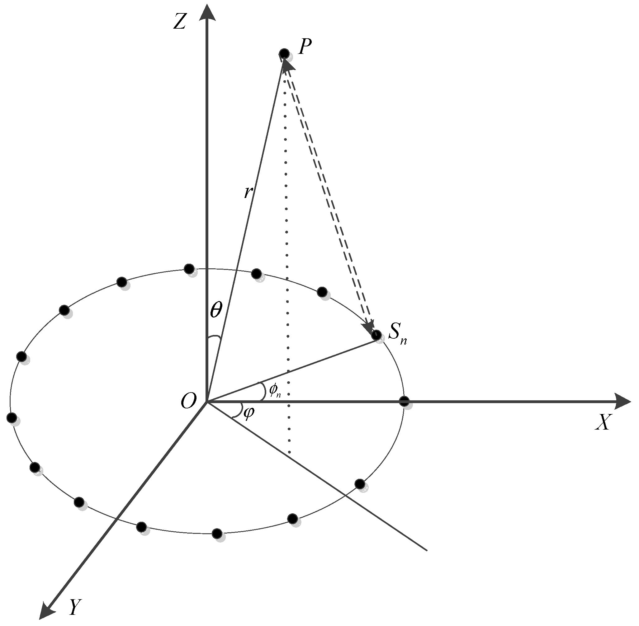
2. Echo Model Based on UCA

The geometry of vortex EM wave detection based on a UCA is illustrated in Figure 1. The vortex EM waves with different orders are generated by a UCA, which comprises $N$ antennas with the radius $a$, and the center of the UCA is set at the coordinate origin $O$. The $n$th element of the UCA is denoted by $S_n$, and the transmitting signal from $S_n$ is denoted by $s_n(t)$. As known from Refs. [2,3], $S_n$ is modulated with the phase ${\varphi }_n$ and ${\varphi }_n=\frac{2\pi }{N}n$; therefore, the transmitting signal $s_n(t)$ can be expressed as

$$\begin{array}{l}{s}_n(t)=\mathrm{rect}[t/T]\bullet \exp (j\pi K{t}^2+j2\pi f_{c}t)\bullet \exp (j{\varphi }_n\alpha )\\ \hspace{1em}\hspace{0.17em}\hspace{0.17em}\hspace{0.17em}=s(t)\exp (j{\varphi }_n\alpha )\end{array}$$

(1)

where $\mathrm{rect}[\bullet ]$ is the function of the pulse signal, $s(t)$ is a linear frequency modulation (LFM) signal and $s(t)=\mathrm{rect}[t/T]\bullet \exp (j\pi K{t}^2+j2\pi f_{c}t)$. $K$ is the LFM rate, $T$ is the transmitted pulse width, $f_c$ is the center frequency of the signal, and $\alpha$ is the order of the OAM mode. Thus, the total signal transmitted by the UCA can be expressed below.

$$s_T(t)={\displaystyle \sum _{n=1}^{N}s(t)\exp (j{\varphi }_n\alpha )}$$

(2)

Assume $P(r_p,{\theta }_p,{\phi }_p)$ is an arbitrary scatterer in space, where $r_p$ is the range between point $P$ and the coordinate origin $O$, and ${\theta }_p$ and ${\phi }_p$ represent the elevation and azimuth of $P$, respectively. Based on the geometry, as shown in Figure 1, the echo of the scatterer $P$ received by the UCA can be expressed as [9]:

$$s_{\mathrm{in}}(t,\alpha )=\sigma s(t-{\tau }_p)\times J_{\alpha }{}^2(ka\sin {\theta }_p)\times \exp (j2\alpha {\phi }_p)$$

(3)

where ${\tau }_p$ is the time delay and ${\tau }_p\approx \frac{2r_p}{c}$; $\sigma$ is the normalized scattering coefficient; $c$ is the speed of light; $k$ is the wavenumber; $J_{\alpha }(•)$ is the Bessel function of the first kind of order $\alpha$; and $\alpha$ is an integer number. According to Refs. [19,20], the signal transmitted by elements of the UCA can be phase-modulated and also amplitude-modulated; then, the vortex EM wave with fractional order is obtained. Similarly, the echo of scatterer $P$ for fractional order can be given by

$$s_{fr}(t,\alpha )=\sigma s(t-{\tau }_p)\times J_{\alpha }{}^2(ka\sin {\theta }_p)\times \exp (j2\alpha {\phi }_p)$$

(4)

where the value of $\alpha$ is the fraction in Equation (4). Assuming the target comprises $M$ independent scatterers, the echo of the target can be uniformly expressed as below from the description in Equations (3) and (4)

$$s_M(t,\alpha )={\displaystyle \sum _{p=1}^M{\sigma }_{p}s(t-{\tau }_p)\times J_{\alpha }{}^2(ka\sin {\theta }_p)\times \exp (j2\alpha {\phi }_p)}$$

(5)

Assuming the range of the integer-order OAM mode is $[-l,l]$, and the fractional order OAM modes separately are ${\alpha }_{1/2}=\frac{1}{2}$ and ${\alpha }_{-1/2}=-\frac{1}{2}$. Then, the echo signals with different kinds of orders in matrix form can be described as

$$\mathit{S}={[s_M(t,{\alpha }_1),s_M(t,{\alpha }_2),\hspace{0.17em}\dots \hspace{0.17em},s_M(t,{\alpha }_{2l}),s_M(t,{\alpha }_{1/2}),s_M(t,{\alpha }_{-1/2})]}^T$$

(6)

where $[{\alpha }_1,{\alpha }_1,\cdots {\alpha }_{2l}]$ corresponds to the range of the OAM-mode order $[-l,l]$.

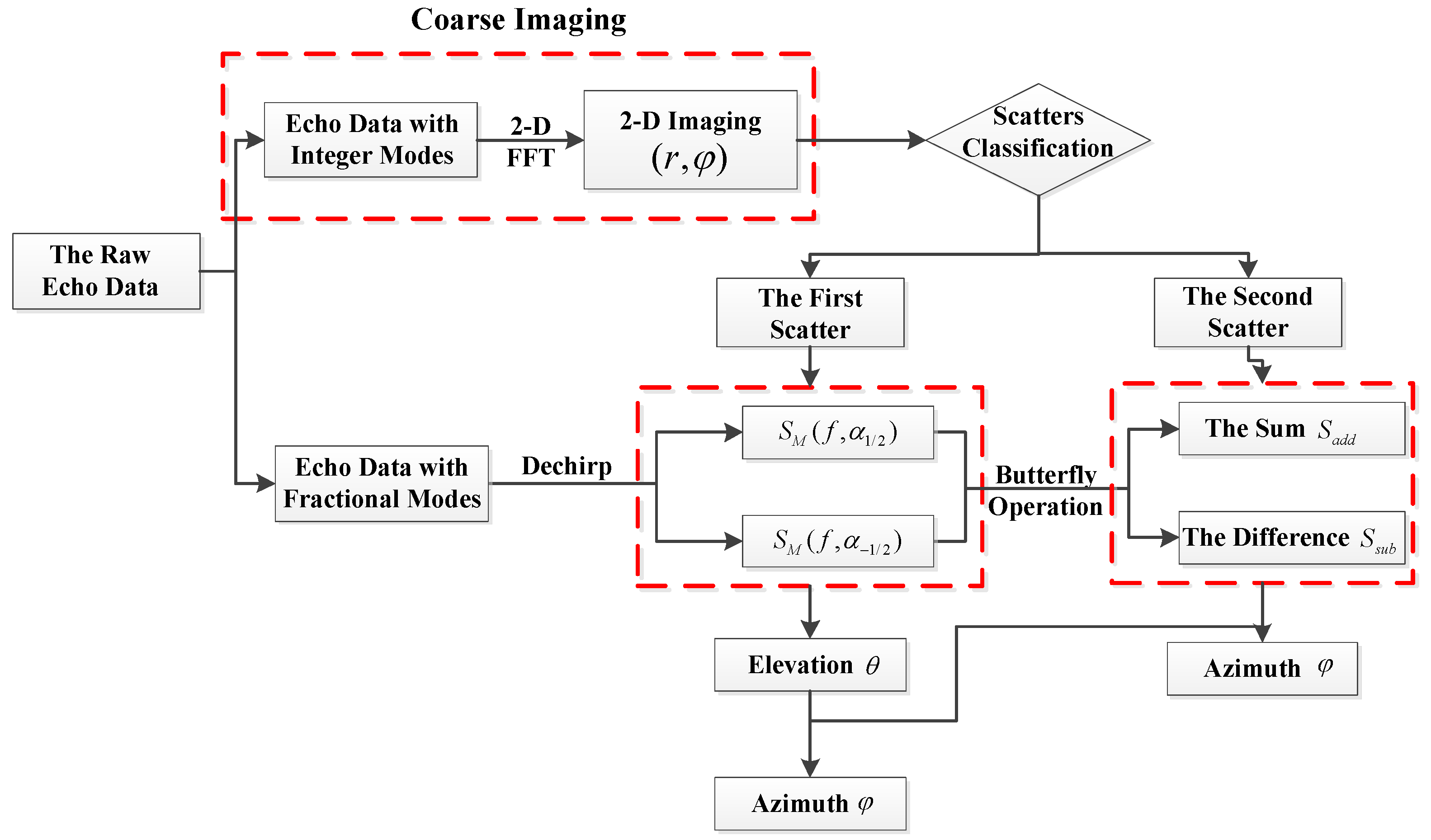
3. Three-Dimensional Imaging Algorithm

According to Equation (6), the echo signal in $\mathit{S}$ can be expressed as a matrix, and the imaging of the range and azimuth can be obtained from $\mathit{S}$ by the two-dimensional FFT method. However, it has no ability to obtain the elevation of the target. In order to obtain the elevation resolution and realize the three-dimensional reconstruction of the target, the signals with integer order in $\mathit{S}$ are operated by two-dimensional FFT first. The information on the range and azimuth of the target can be obtained, which is called coarse imaging. Secondly, the scatterers are classified into two types according to the range distribution from the results of coarse imaging. Finally, the elevation of two kinds of scatterers can be solved by utilizing the echo with $\pm \frac{1}{2}$ OAM orders. As a result, the three-dimensional reconstruction is realized.

3.1. Coarse Imaging

The echo signals with integer order are selected to form a new matrix ${\mathit{S}}_{\mathrm{in}}$, and ${\mathit{S}}_{\mathrm{in}}$ is defined as ${\mathit{S}}_{\mathrm{in}}={[s_M(t,{\alpha }_1),.....,s_M(t,{\alpha }_{2l})]}^T$. The center point $P_c$ of the target is initially set as the reference point, and then the echo of $P_c$ with integer order can be expressed as

$${\mathit{S}}_{P_c}={[s_{P_c}(t,{\alpha }_1),s_{P_c}(t,{\alpha }_2),\hspace{0.17em}\dots \hspace{0.17em},s_{P_c}(t,{\alpha }_{2l})]}^T$$

(7)

where $s_{P_c}(t,{\alpha }_n)$ is the echo of $P_c$ with $n$th order. The range of the target can be obtained through range imaging with matched filtering for ${\mathit{S}}_{\mathrm{in}}$, and the processed signal can be expressed as

$${\mathit{S}}_{Match}={[s_{Match}(t,{\alpha }_1),s_{Match}(t,{\alpha }_2),\hspace{0.17em}\dots \hspace{0.17em},s_{Match}(t,{\alpha }_{2l})]}^T$$

(8)

where $s_{Match}(t,{\alpha }_n)$ can be expressed as

$$s_{Match}(t,{\alpha }_n)=s_M(t,{\alpha }_n)\ast s^{*}{}_{P_c}(-t,{\alpha }_n)={\displaystyle \sum _{p=1}^M{\sigma }_{p}ps{f}_t(t-{\tau }_p)\exp (j{\alpha }_n{\phi }_p)}$$

(9)

where $ps{f}_t(\bullet )$ is the point-spread function in the time domain.

Then, ${\mathit{S}}_{Match}$ can be processed in terms of the OAM mode by FFT to obtain the azimuth image. With the above processing, the results of coarse imaging can be obtained. The scatterers are classified into two types by the distribution of scatterers in the range bin; that is, if there is only one scatterer in the range bin, the scatterer is defined as the first kind scatterer and denoted by $P^{\prime }$; if more than one scatterer exists in the same range bin, these scatterers are defined as the second kind scatterers denoted by $P^{″}$. Assume the number of $P^{\prime }$ is $L_1$ and the number of $P^{″}$ is $L_2$, then, $L_1$ and $L_2$ must satisfy $L_1+L_2=M$.

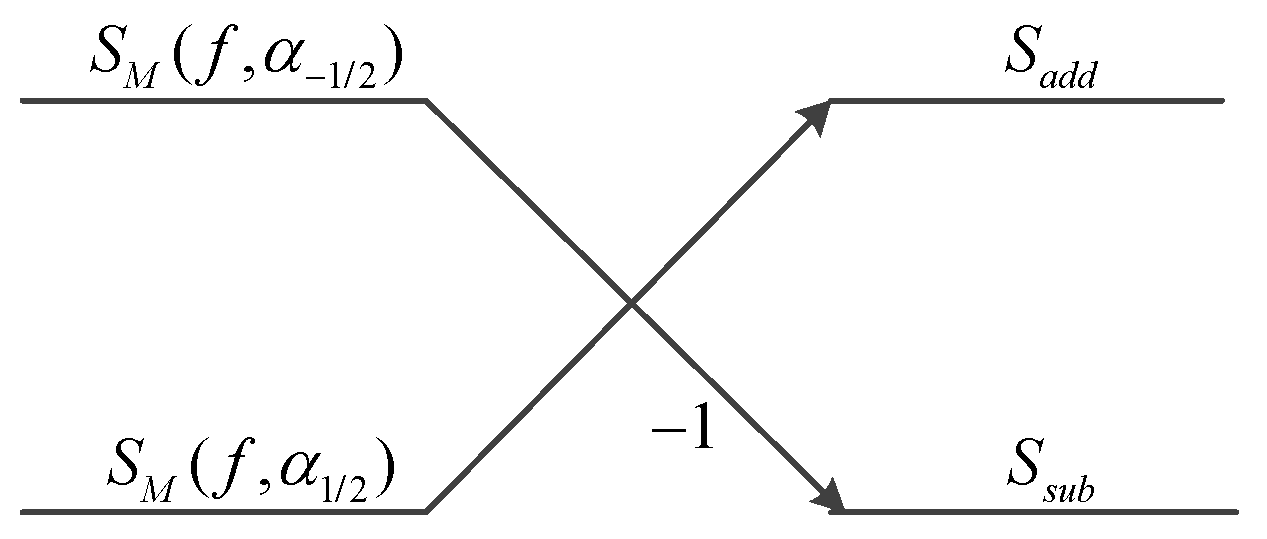
3.2. Three-Dimensional Imaging

Through coarse imaging, only two-dimensional information can be obtained. In order to achieve the elevation reconstruction, the signal matrix ${\mathit{S}}_{fr}$ with $\pm \frac{1}{2}$ orders is established, which is defined as ${\mathit{S}}_{fr}={[s_M(t,{\alpha }_{1/2}),s_M(t,{\alpha }_{-1/2})]}^T$. According to Refs. [40,41], when $\alpha$ equals $\pm \frac{1}{2}$, the first type of Bessel function can be expressed as

$$J_{-\frac{1}{2}}(z)=\sqrt{\frac{2}{\pi z}}\cos (z)$$

(10)

$$J_{\frac{1}{2}}(z)=\sqrt{\frac{2}{\pi z}}\sin (z)$$

(11)

After the operation of matched filtering, the fractional order echo ${\mathit{S}}_{fr}$ can be further expressed as

$$\begin{array}{l}{s}_M(t,{\alpha }_{1/2})={\displaystyle \sum _{p=1}^M{\sigma }_{p}s(t-{\tau }_p)\times J_{{\alpha }_{1/2}}{}^2(ka\sin {\theta }_p)\times \exp (j2{\alpha }_{1/2}{\phi }_p)}\\ \hspace{1em}\hspace{1em}\hspace{1em}={\displaystyle \sum _{p=1}^M\frac{2{\sigma }_{p}s(t-{\tau }_p)}{\pi ka\sin {\theta }_p}{\cos }^2(ka\sin {\theta }_p)\times \exp (-j{\phi }_p)}\end{array}$$

(12)

$$\begin{array}{l}{s}_M(t,{\alpha }_{-1/2})={\displaystyle \sum _{p=1}^M{\sigma }_{p}s(t-{\tau }_p)\times J_{{\alpha }_{-1/2}}{}^2(ka\sin {\theta }_p)\times \exp (j2{\alpha }_{-1/2}{\phi }_p)}\\ \hspace{1em}\hspace{1em}\hspace{1em}={\displaystyle \sum _{p=1}^M\frac{2{\sigma }_{p}s(t-{\tau }_p)}{ka\sin {\theta }_p}{\sin }^2(ka\sin {\theta }_p)\times \exp (j{\phi }_p)}\end{array}$$

(13)

The transmitting signal is set as the reference signal. De-chirping and FFT are used to process ${\mathit{S}}_{fr}$; therefore, the processed ${\mathit{S}}_{fr}$ can be expressed as

$$\begin{array}{l}{S}_M(f,{\alpha }_{1/2})={\displaystyle \sum _{p=1}^M\frac{2{\sigma }_p{\cos }^2(ka\sin {\theta }_p)}{\pi ka\sin {\theta }_p}\exp (-j{\phi }_p)\times T\sin \mathrm{c}[T(f+2\frac{K}{c}{R}_{\Delta })]}\\ \hspace{1em}\hspace{1em}\hspace{1em}\hspace{1em}\hspace{1em}\hspace{1em}\hspace{1em}\times \exp (j\frac{4\pi f_c}{c}{R}_{\Delta })\end{array}$$

(14)

$$\begin{array}{l}{S}_M(f,{\alpha }_{-1/2})={\displaystyle \sum _{p=1}^M\frac{2{\sigma }_p{\sin }^2(ka\sin {\theta }_p)}{\pi ka\sin {\theta }_p}\exp (j{\phi }_p)\times T\sin \mathrm{c}[T(f+2\frac{K}{c}{R}_{\Delta })]}\\ \hspace{1em}\hspace{1em}\hspace{1em}\hspace{1em}\hspace{1em}\hspace{1em}\hspace{1em}\times \exp (j\frac{4\pi f_c}{c}{R}_{\Delta })\end{array}$$

(15)

where $R_{\Delta }=r_p-r_{ref}$ and $r_{ref}$ is the range between the reference point and transmitters. Due to the transmitting signal being set as the reference signal, therefore, $r_{ref}=0$ and $R_{\Delta }=r_p$. From the properties of the sinc function, the information of the target range can be obtained by the operation with de-chirping and FFT successively. If the scatterers are in different range bins, each peak can represent only one scatterer. According to Equations (14) and (15), the amplitude of each scatterer on a one-dimensional range profile with $\pm \frac{1}{2}$ order can be expressed as

$$A_{P,{\alpha }_{1/2}}=T\frac{2{\sigma }_p}{\pi ka\sin {\theta }_p}\sin \mathrm{c}[T(f+2\frac{K}{c}{R}_{\Delta })]{\cos }^2(ka\sin {\theta }_p)$$

(16)

$$A_{P,{\alpha }_{-1/2}}=T\frac{2{\sigma }_p}{\pi ka\sin {\theta }_p}\sin \mathrm{c}[T(f+2\frac{K}{c}{R}_{\Delta })]{\sin }^2(ka\sin {\theta }_p)$$

(17)

Divide the amplitude $A_{P,{\alpha }_{-1/2}}$ by $A_{P,{\alpha }_{1/2}}$ to yield the following:

$$v_p=\frac{A_{P,{\alpha }_{-1/2}}}{A_{P,{\alpha }_{1/2}}}=\frac{{\sin }^2(ka\sin {\theta }_p)}{{\cos }^2(ka\sin {\theta }_p)}={\tan }^2(ka\sin {\theta }_p)$$

(18)

Equation (17) can be further expressed as

$${\theta }_p=arc\sin (\frac{\arctan (\sqrt{v_p})}{a}\frac{c}{2\pi f_c})$$

(19)

The target elevation information corresponding to different range bins can be obtained through Equation (19). Although the two-dimensional imaging result of the target is obtained by coarse imaging, the target azimuth still needs to be solved from fine imaging by utilizing the echo signal with $\pm \frac{1}{2}$ OAM modes. The signals expressed in Equations (14) and (15) are processed with the butterfly operation, which is shown in Figure 2.

In Figure 2, the sum of $S_M(f,{\alpha }_{1/2})$ and $S_M(f,{\alpha }_{-1/2})$ is denoted by $S_{add}=S_M(f,{\alpha }_{1/2})+S_M(f,{\alpha }_{-1/2})$, and the difference of $S_M(f,{\alpha }_{1/2})$ and $S_M(f,{\alpha }_{-1/2})$ is denoted by $S_{sub}=S_M(f,{\alpha }_{1/2})-S_M(f,{\alpha }_{-1/2})$. The signal $S_{add}$ can be further expressed as

$$\begin{array}{l}{S}_{add}=S_M(f,{\alpha }_{1/2})+S_M(f,{\alpha }_{-1/2})\\ \hspace{1em}\hspace{0.17em}\hspace{0.17em}={\displaystyle \sum _{p=1}^{M}T\frac{2{\sigma }_p}{\pi ka\sin {\theta }_p}\sin c[T(f+2\frac{K}{c}{R}_{\Delta })]}\exp (j\frac{4\pi f_c}{c}{R}_{\Delta })\\ \hspace{1em}\hspace{1em}\hspace{1em}\hspace{1em}\times [\exp (j{\phi }_p){\sin }^2(ka\sin {\theta }_p)+\exp (-j{\phi }_p){\cos }^2(ka\sin {\theta }_p)]\end{array}$$

(20)

Assume $s_p=\exp (j{\phi }_p){\sin }^2(ka\sin {\theta }_p)+\exp (-j{\phi }_p){\cos }^2(ka\sin {\theta }_p)$, and exponential term $\exp (j{\phi }_p)$ can be expanded by utilizing the Euler formula. Then, $s_p$ can be further expressed as

$$\begin{array}{l}{s}_p=\cos {\phi }_p[{\sin }^2(ka\sin {\theta }_p)+{\cos }^2(ka\sin {\theta }_p)]-j\sin {\phi }_p[{\sin }^2(ka\sin {\theta }_p)-{\cos }^2(ka\sin {\theta }_p)]\\ \hspace{1em}=\cos {\phi }_p-j\sin {\phi }_p\cos (2ka\sin {\theta }_p)\end{array}$$

(21)

According to Equation (20), Equation (19) can be further represented as

$$\begin{array}{l}{S}_{add}={\displaystyle \sum _{p=1}^{M}T\frac{2{\sigma }_p}{\pi ka\sin {\theta }_p}\sin c[T(f+2\frac{K}{c}{R}_{\Delta })]}\exp (j\frac{4\pi f_c}{c}{R}_{\Delta })\\ \hspace{1em}\hspace{1em}\hspace{1em}\hspace{1em}\times [\cos {\phi }_p-j\sin {\phi }_p\cos (2ka\sin {\theta }_p)]\end{array}$$

(22)

From Equation (21), if only the amplitude of the range image is considered, then the amplitude in different range bins can be expressed as

$$\begin{array}{l}{v}_{p,add}=T\frac{2{\sigma }_p}{\pi ka\sin {\theta }_p}\sin c[T(f+2\frac{K}{c}{R}_{\Delta })]\\ \hspace{1em}\hspace{1em}\hspace{1em}\hspace{0.17em}\times \sqrt{{\cos }^2{\phi }_p+{\sin }^2{\phi }_p{\cos }^2(2ka\sin {\theta }_p)}\end{array}$$

(23)

Similarly, $S_{sub}$ can be expressed as

$$\begin{array}{l}{S}_{sub}={\displaystyle \sum _{p=1}^{M}T\frac{2{\sigma }_p}{\pi ka\sin {\theta }_p}\sin c[T(f+2\frac{K}{c}{R}_{\Delta })]}\exp (j\frac{4\pi f_c}{c}{R}_{\Delta })\\ \hspace{1em}\hspace{1em}\hspace{1em}\hspace{1em}\times [j\sin {\phi }_p-\cos {\phi }_p\cos (2ka\sin {\theta }_p)]\end{array}$$

(24)

The amplitude of signal $S_{sub}$ in different distance units can be expressed as

$$\begin{array}{l}{v}_{p,sub}=T\frac{2{\sigma }_p}{\pi ka\sin {\theta }_p}\sin c[T(f+2\frac{K}{c}{R}_{\Delta })]\\ \hspace{1em}\hspace{1em}\hspace{1em}\hspace{0.17em}\times \sqrt{{\cos }^2{\phi }_p{\cos }^2(2ka\sin {\theta }_p)+{\sin }^2{\phi }_p}\end{array}$$

(25)

Then, we have

$$h_p={(\frac{v_{p,add}}{v_{p,sub}})}^2=\frac{{\sin }^2{\phi }_p{\cos }^2(2ka\sin {\theta }_p)+{\cos }^2{\phi }_p}{{\cos }^2{\phi }_p{\cos }^2(2ka\sin {\theta }_p)+{\sin }^2{\phi }_p}$$

(26)

The elevation has been solved by Equation (18); thus, the azimuth of the target can be derived from Equation (25) as

$${\phi }_p=\arctan (\sqrt{\frac{1-h_p{\cos }^2(2ka\sin {\theta }_p)}{h_p-{\cos }^2(2ka\sin {\theta }_p)}})$$

(27)

Therefore, according to Equations (18) and (26), the azimuth and elevation of the target can be obtained by processing the echo signal with fractional OAM modes. However, the above signal processing flow is based on the premise that the scatterers are distributed in different range bins. It means that the above three-dimensional imaging processing is applicable for the first kind of scatterers. If the scatterers belong to the second kind, there will be no resolution of the azimuth and elevation with the above processing. In order to obtain the elevation of the second kind of scatterers, the azimuth ${\phi }_p$ from the result of the coarse imaging needs to be used. Equation (27) can be further described as

$$\sin {\theta }_p=\arccos (\sqrt{\frac{1-h_p{\tan }^2{\phi }_p}{h_p-{\tan }^2{\phi }_p}})/2ka$$

(28)

Equation (28) shows that the elevation of different scatterers in the same range bin can be solved by using the information from coarse imaging, and then the second kind of scatterers can be three-dimensional reconstructed. Therefore, the three-dimensional reconstruction of the target can be realized from Equations (19), (27) and (28). It must be mentioned that the amplitude of the range imaging may be easily disturbed and unstable by many factors, such as noise. In fact, the range information can be obtained from just one pulse, and the radar transmits many pulses per second; thus, many groups of range images can be obtained per second. The average amplitude of range images can be used to solve the elevation and azimuth in order to reduce the effect of noise.

To sum up, the flow of the three-dimensional imaging method based on the vortex EM wave with integer- and fractional-order OAM modes are shown in Figure 3, and the steps can be described as follows:

Step (1): the matrix of the echo signal $\mathit{S}$ is established based on a UCA with integer and fractional orders.

Step (2): the echo signal ${\mathit{S}}_{in}$ with integer orders is processed by FFT, and coarse imaging, in terms of the range and azimuth, can be obtained.

Step (3): according to the result of coarse imaging, the scatterers are classified as the first or second kind of scatterers.

Step (4): the echo signal ${\mathit{S}}_{fr}$ with fractional orders is processed with the butterfly operation, then $S_{add}$ and $S_{sub}$ can be obtained.

Step (5): the elevation and azimuth of the first kind of scatterers are solved through Equations (18) and (26), and the three-dimensional reconstruction of this kind of scatterer is realized.

Step (6): by using the azimuth information of coarse imaging, the elevation of the second kind of scatterer is solved through Equation (28), and the three-dimensional reconstruction of this kind of scatterer is realized.

Step (7): the results in Steps 5 and 6 are fused to realize the three-dimensional reconstruction of the radar target.

According to the above steps, the three-dimensional reconstruction of the radar target can be realized. Next, let us discuss the resolution of the target range, azimuth and elevation of the proposed method. The proposed method realizes range imaging by using FFT. Therefore, according to Ref. [26], the range resolution depends on the point-spread function (PSF) and is inversely proportional to the signal bandwidth $B$, which can be expressed as

$${\rho }_r=\frac{c}{2B}$$

(29)

Due to the different kinds of scatterers, there are also differences in solving the azimuth and elevation of the scatterers. For the second kind of scatterers, the azimuth imaging is achieved by FFT in terms of the OAM mode. Then, the resolution can be expressed as

$${\rho }_{\phi }=\frac{\pi }{\Delta \alpha }$$

(30)

where $\Delta \alpha$ is the range of the OAM mode order. The elevations of the second kind of scatterers are obtained by Equation (27), which is solved through the arcsine function. Assuming the resolution of elevation is ${\rho }_{\theta }$, the calculation errors of elevation $\Delta x$ satisfy:

$$\Delta x\le \sin (\theta +{\rho }_{\theta })-\sin \theta$$

(31)

According to the properties of trigonometric functions, the value of $\Delta x$ is different in the areas of $[0,\frac{\pi }{2}]$, which is shown in Figure 4. Figure 4 shows the relationship of the calculation errors and $\Delta \theta$, and $\Delta \theta$ is the elevation resolution by the reconstruction algorithm in this paper. It is obvious that $\Delta x$ decreases with increasing elevation $\theta$.

For the first kind of scatterers, the elevation is solved from Equation (18) by utilizing the properties of the Bessel function with fractional order. By comparing Equation (18) with Equation (28), the elevation of the first kind of scatterer is also obtained by an arcsine function, and thus it must satisfy Equation (31). However, the azimuth still needs to be solved by Equation (27), which is obtained by an arctan function. Assuming the azimuth resolution is ${\rho }_{\phi }$, the calculation error of elevation $\Delta y$ will satisfy

$$\Delta y\le \tan (\phi +{\rho }_{\phi })-\tan \phi$$

(32)

According to the properties of trigonometric functions, the value of $\Delta y$ is also different in the areas of $[0,\frac{\pi }{2}]$. Figure 5 shows the relationship between the calculation errors and $\Delta \phi$, and $\Delta \phi$ is the azimuth resolution by the reconstruction algorithm in this paper. It is obvious that $\Delta y$ increases with the increasing azimuth $\phi$.

The requirement of $\Delta x$ and $\Delta y$ are compared with the same resolution, which is shown in Figure 6, and $\Delta$ is defined as a calculation error of the azimuth or elevation. It can be found that the requirement of $\Delta y$ is significantly higher than the requirement of $\Delta x$.

According to the imaging flow for the first kind of scatterers, the azimuth can be obtained not only from the coarse imaging but also from Equation (27). The resolution of azimuth depends on different factors in these two methods. In the coarse imaging method, the resolution satisfies Equation (30) and depends on the range of OAM modes; while in the second method, it satisfies Equation (32) and depends on the calculation errors. In certain conditions, especially when the azimuth angle is relatively large, the azimuth resolution in the coarse imaging method will be lower than the second method.

The accuracy of target reconstruction is not only related to the resolution of elevation and azimuth but also related to the signal-to-noise ratio (SNR). The elevation and azimuth of the target are obtained by calculating the amplitude term of the one-dimensional range profile of the echo signal; therefore, the echo signal with fractional order can be expressed as:

$$s_M^{\prime }(t,{\alpha }_{1/2})=s_M(t,{\alpha }_{1/2})+n(t)$$

(33)

$$s_M^{\prime }(t,{\alpha }_{-1/2})=s_M(t,{\alpha }_{-1/2})+n(t)$$

(34)

where $n(t)$ is Gaussian white noise. According to the properties of Gaussian white noise, Gaussian white noise has values in all frequencies, and thus, the amplitude term can be expressed in Equations (34) and (35) after de-chirping and the FFT operation.

$$A_{P,{\alpha }_{1/2}}^{\prime }=A_{P,{\alpha }_{1/2}}+N_{P,{\alpha }_{1/2}}(f)$$

(35)

$$A_{P,{\alpha }_{-1/2}}^{\prime }=A_{P,{\alpha }_{-1/2}}+N_{P,{\alpha }_{-1/2}}(f)$$

(36)

where $N_{P,{\alpha }_{1/2}}(f)$ and $N_{P,{\alpha }_{-1/2}}(f)$ are the amplitudes of the Gaussian white noise of each scatterer with $\pm \frac{1}{2}$ order; thus, the $v_p$ is expressed as:

$$v_p^{\prime }=\frac{A_{P,{\alpha }_{-1/2}}^{\prime }}{A_{P,{\alpha }_{1/2}}^{\prime }}=v_p+v_{randn}$$

(37)

where $v_{randn}$ is a random value that satisfies the Gaussian distribution, and it is known that the SNR can be approximated as:

$$SNR=20\log (v_p/v_{randn})$$

(38)

It can be found that the value of $v_{randn}$ will increase as the SNR decreases from Equation (38). It also leads to a decrease in the algorithm’s reconstruction accuracy as the SNR decreases.

4. Simulation

In this section, the performance of the proposed method is validated by simulations. The UCA comprises 50 elements with a radius of 0.1 m, and the center of the UCA is set at the origin. The integer OAM mode during this is $[-20,20]$, and the fractional OAM modes are $\frac{1}{2}$ and $-\frac{1}{2}$, respectively. The LFM signal is set as a transmitting signal; the center of frequency is 10 GHz; and the bandwidth of the signal is 100 MHz. There are seven independent scatterers on the target, and the coordinates of these scatterers are listed in

Table 1. The coordinates of scatterers.

The Index of Scatterer	X (m)	Y (m)	Z (m)	The Index of Scatterer	X (m)	Y (m)	Z (m)
$P_1$	80	100	250	$P_5$	120	150	120
$P_2$	140	100	200	$P_6$	220	80	60
$P_3$	150	150	190	$P_7$	220	60	80
$P_4$	120	120	180

and shown in Figure 7.

4.1. Processing of Coarse Imaging

The echo signal ${\mathit{S}}_{in}$ is processed by FFT in terms of the frequency and OAM mode, respectively, and the results of the range and azimuth are shown in Figure 8. According to the conversion formula of the Cartesian coordinate system to a Spherical coordinate system, the scatterers in Table 1 can be written in the Spherical coordinate system in

Table 2. The distribution of scatterers in the Spherical coordinate system.

The Index of Scatterer	R(m)	$\mathit{\phi }$ (/$\mathit{\pi }$)	$\mathit{\theta }$ (/$\mathit{\pi }$)	The Index of Scatterer	R(m)	$\mathit{\phi }$ (/$\mathit{\pi }$)	$\mathit{\theta }$ (/$\mathit{\pi }$)
$P_1$	289.89	0.29	0.17	$P_5$	226.49	0.29	0.32
$P_2$	263.81	0.19	0.23	$P_6$	241.66	0.11	0.42
$P_3$	284.78	0.25	0.27	$P_7$	241.66	0.08	0.39
$P_4$	247.38	0.25	0.24

.

Figure 8 shows the range and azimuth imaging of scatterers. It means the distribution of the scatterers can be obtained by coarse imaging. According to the results of coarse imaging, the scatterers $P_6$ and $P_7$ are located in the same range bin, and the scatterers $P_1$~$P_5$ distribute in different range bins, respectively. According to the classification criteria for the scatterers defined in this article, the scatterers $P_1$~$P_5$ are classified as the first kind of scatterers and $P_6$ and $P_7$ are classified as the second kind of scatterers.

4.2. Processing of Signal with Fractional OAM Mode

The scatterers are partitioned into two kinds after coarse imaging. In order to obtain the elevation information, the echo signal with $\pm \frac{1}{2}$ OAM modes is processed. The de-chirping and the butterfly operation are used successively, and then the results of $S_{add}$ and $S_{sub}$ are shown in Figure 9, where Figure 9a,b show the range imaging of $S_{add}$ and $S_{sub}$, respectively. It can be found that the distribution of the scatterers in Figure 9a is the same as that in Figure 8a; however, the amplitudes of the range image peaks are different. By utilizing this difference and the characteristic of the Bessel function, the elevation of the scatterers can be obtained.

4.3. Reconstruction of the First Kind of Scatterers

The elevation and azimuth of the first kind of scatterers can be obtained from Equations (18) and (26). In order to improve the reconstruction accuracy and reduce the effect of noise, multi-pulses are used to obtain the average of the amplitude of range imaging. Assume that the signal-to-noise ratio (SNR) is 5 dB, the pulse repetition frequency (PRF) is 1000, and the average amplitude of 1000-times-range imaging is used. The results of two-dimensional imaging, in terms of the elevation and azimuth, are shown in Figure 10, where the red color represents the ideal model of scatterers, and the blue color represents the rebuilt scatterers. Figure 10a shows the imaging of all the scatterers, and Figure 10b shows the imaging result of the first kind of scatterers. From the results shown in Figure 10, the imaging method for the first kind of scatterers can realize the accurate reconstruction of $P_1$~$P_5$. However, for the second kind of scatterers $P_6$ and $P_7$, only one scatterer can be rebuilt, and the solved information is also not the real coordinate of the scatterers.

The reconstruction method for the first kind of scatterers proposed in this paper utilizes the amplitude of the range imaging; therefore, it is necessary to consider the performance of the proposed method under the different SNRs. Assuming the range of SNR is from −10 dB to 15 dB, the average deviation and average variance of elevation and azimuth are calculated and recorded as shown in Figure 11, where the red color represents the error of elevation and the blue color represents the error of azimuth. When the SNR is higher than 5 dB, the reconstruction method has good performance, and the errors are stable. The average deviation and average variance of elevation are no more than $0.06\pi$ and $0.005\pi$, respectively. The average deviation and average variance of azimuth are no more than $0.03\pi$ and $0.001\pi$, respectively. Compared to the reconstruction error of elevation and azimuth under the same SNR, it can be found that the estimation accuracy of the azimuth is obviously better than the elevation.

When the elevation and azimuth have been solved, the three-dimensional reconstruction can be realized. Figure 12 shows the three-dimensional imaging of $P_1$~$P_5$ when the SNR is 5 dB. The effectiveness of the proposed method for the first kind of scatterers is verified.

4.4. Reconstruction of the Second Kind of Scatterers

From the simulation in Section 4.3, it can be found that the method for the first kind of scatterers is not suitable for the second kind of scatterers. The azimuth of $P_6$ and $P_7$, obtained from the coarse imaging result, should be fully utilized for the three-dimensional reconstruction; thus, the azimuth results are used to solve the elevation of $P_6$ and $P_7$ through Equation (27). Assuming the SNR is 5 dB, the two-dimensional imaging result in the elevation and azimuth domains are shown in Figure 13. $P_6$ and $P_7$ can be distinguished in the elevation domain in Figure 13.

The reconstruction method for the second kind of scatterers also utilizes the amplitude of range imaging result; thus, the effect of the SNR on the performance of the method must be considered. Assuming the range of the SNR is from 0 dB to 15 dB, the average deviation, average variance and average mean square error (MSE) of elevation are calculated and recorded, as shown in Figure 14. When the SNR is higher than 5 dB, the reconstruction method has good performance, and the errors are stable. The average deviation and average variance of elevation are no more than $0.06\pi$ and $0.005\pi$, respectively. The average MSE is no more than 0.002$\pi$.

4.5. Three-Dimensional Imaging of the Target

According to the imaging results in Section 4.3 and Section 4.4, the two kinds of scatterers can be combined to recover the three-dimensional imaging result of the target, which is shown in Figure 15. The method proposed in this paper based on integer and fractional orders has good performance in the reconstruction of the target, and the three-dimensional coordinates of scatterers $P_1$~$P_7$ are accurately reconstructed.

In order to further validate the three-dimensional imaging algorithm proposed in this paper, the three-dimensional imaging algorithm proposed is used to image the simplified scattering model of the aircraft, and the three-dimensional imaging result is shown in Figure 16. It can be seen that the aircraft scattering point model is well reconstructed from Figure 16.

5. Conclusions

This paper studied the three-dimensional imaging method based on the vortex EM wave with integer- and fractional-order OAM modes. Three-dimensional imaging is realized through a two-step imaging process. Moreover, the resolution of the elevation and azimuth and the effects of the SNR are analyzed, respectively. The simulation results show that the proposed method can effectively reconstruct the three-dimensional image of the target. The biggest advantage of this method is that the three-dimensional imaging no longer depends on the aperture by relative motion between the radar and target or the antenna array itself. This means that the imaging method proposed in this article can meet the real-time imaging requirements for moving targets, such as security, low-speed aerospace target detection and so on. This method provides a new technical approach for three-dimensional imaging based on vortex EM waves.

References

1. Allen, L.; Beijersbergen, M.W.; Spreeuw RJ, C.; Woerdman, J.P. Orbital angular momentum of light and the transformation of Laguerre-Gaussian laser modes. Phys. Rev. A 1992, 45, 8185–8189. [Google Scholar] [CrossRef] [PubMed]
2. Jackson, J.D. Classical Electrodynamics, 3rd ed.; Wiley-VCH: Weinheim, Germany, 1999; p. 832. ISBN 0-471-30932-X. [Google Scholar] [CrossRef]
3. Liu, K.; Li, X.S.; Wang, H.Q.; Cheng, Y.Q. The Advances of Vortex Electromagnetic Wave in Radar Applications. Acta Electron. Sin. 2018, 46, 2283–2290. [Google Scholar] [CrossRef]
4. Thidé, B.; Then, H.; Sjöholm, J.; Palmer, K.; Bergman, J.; Carozzi, T.D.; Istomin, Y.N.; Ibragimov, N.H.; Khamitova, R. Utilization of Photon Orbital Angular Momentum in the Low-Frequency Radio Domain. Phys. Rev. Lett. 2007, 99, 087701. [Google Scholar] [CrossRef] [Green Version]
5. Tamburini, F.; Mari, E.; Sponselli, A.; Thidé, B.; Bianchini, A.; Romanato, F. Encoding many channels on the same frequency through radio vorticity: First experimental test. New J. Phys. 2012, 14, 033001. [Google Scholar] [CrossRef] [Green Version]
6. Edfors, O.; Johansson, A.J. Is Orbital Angular Momentum (OAM) Based Radio Communication an Unexploited Area? IEEE Trans. Antennas Propag. 2012, 60, 1126–1131. [Google Scholar] [CrossRef] [Green Version]
7. Tamagnone, M.; Craeye, C.; Perruisseau-Carrier, J. Comment on ‘Encoding many channels on the same frequency through radio vorticity: First experimental test’. arXiv 2012, arXiv:1210.5365. [Google Scholar] [CrossRef]
8. Sun, X.H.; Li, Q.; Pang, D.X.; Zeng, Z.M. New Research Progress of the Orbital Angular Momentum Technology in Wireless Communication: A Survey. Acta Electron. Sin. 2015, 43, 2305–2314. [Google Scholar]
9. Guo, G.; Hu, W.; Du, X. Electromagnetic vortex based radar target imaging. J. Natl. Univ. Def. Technol. 2013, 35, 71–76. [Google Scholar]
10. Liu, K.; Cheng, Y.; Li, X.; Wang, H.; Qin, Y.; Jiang, Y. Study on the theory and method of vortex-electromagnetic-wave-based radar imaging. IET Microw. Antennas Propag. 2016, 10, 961–968. [Google Scholar] [CrossRef]
11. Liu, K.; Cheng, Y.; Yang, Z.; Wang, H.; Qin, Y.; Li, X. Orbital-Angular-Momentum-Based Electromagnetic Vortex Imaging. IEEE Antennas Wirel. Propag. Lett. 2015, 14, 711–714. [Google Scholar] [CrossRef]
12. Liu, K.; Liu, H.; Qin, Y.; Cheng, Y.; Wang, S.; Li, X.; Wang, H. Generation of OAM Beams Using Phased Array in the Microwave Band. IEEE Trans. Antennas Propag. 2016, 64, 3850–3857. [Google Scholar] [CrossRef]
13. Yuan, H.; Chen, Y.J.; Luo, Y.; Liang, J.; Wang, Z.H. A resolution-improved imaging algorithm based on uniform circular array. IEEE Antennas Wirel. Propag. Lett. 2022, 21, 461–465. [Google Scholar] [CrossRef]
14. Liu, K.; Cheng, Y.; Li, X.; Jiang, Y. Passive OAM-Based Radar Imaging with Single-In-Multiple-Out Mode. IEEE Microw. Wirel. Compon. Lett. 2018, 28, 840–842. [Google Scholar] [CrossRef]
15. Liu, K.; Li, X.; Cheng, Y.; Gao, Y.; Fan, B.; Jiang, Y. OAM-Based Multitarget Detection: From Theory to Experiment. IEEE Microw. Wirel. Compon. Lett. 2017, 27, 760–762. [Google Scholar] [CrossRef]
16. Yuan, T.; Wang, H.; Cheng, Y.; Qin, Y. Electromagnetic Vortex-Based Radar Imaging Using a Single Receiving Antenna: Theory and Experimental Results. Sensors 2017, 17, 630. [Google Scholar] [CrossRef] [Green Version]
17. Liu, K.; Li, X.; Gao, Y.; Cheng, Y.; Wang, H.; Qin, Y. High-Resolution Electromagnetic Vortex Imaging Based on Sparse Bayesian Learning. IEEE Sens. J. 2017, 17, 6918–6927. [Google Scholar] [CrossRef]
18. Liu, H.; Liu, K.; Cheng, Y.; Wang, H. Microwave Vortex Imaging Based on Dual Coupled OAM Beams. IEEE Sens. J. 2020, 20, 806–815. [Google Scholar] [CrossRef]
19. Liu, H.; Liu, K.; Cheng, Y.; Wang, H.; Wang, Y. Scattering Characteristics of Vortex Electromagnetic Waves by a Metal Plate. In Proceedings of the 2020 9th Asia-Pacific Conference on Antennas and Propagation (APCAP), Xiamen, China, 4–7 August 2020; pp. 1–2. [Google Scholar] [CrossRef]
20. Liu, K.; Liu, H.; Sha, W.E.I.; Cheng, Y.; Wang, H. Backward Scattering of Electrically Large Standard Objects Illuminated by OAM Beams. IEEE Antennas Wirel. Propag. Lett. 2020, 19, 1167–1171. [Google Scholar] [CrossRef]
21. Yang, L.J.; Sun, S.; Sha, W.E.I. Ultrawideband Reflection-Type Metasurface for Generating Integer and Fractional Orbital Angular Momentum. IEEE Trans. Antennas Propag. 2020, 68, 2166–2175. [Google Scholar] [CrossRef] [Green Version]
22. Chen, R.; Zou, M.; Feng, Q.; Li, J. Generation of OAM Radio Waves Using a Single Antenna in Uniform Circular Motion. In Proceedings of the 2019 8th Asia-Pacific Conference on Antennas and Propagation (APCAP), Incheon, Korea, 4–7 August 2019; pp. 593–594. [Google Scholar] [CrossRef]
23. Chen, R.; Zou, M.; Wang, X.; Tennant, A. Generation and Beam Steering of Arbitrary-Order OAM with Time-Modulated Circular Arrays. IEEE Syst. J. 2021, 15, 5313–5320. [Google Scholar] [CrossRef]
24. Yang, Y.J.; Qiu, C.W. Generation of Optical Vortex Beams, Electromagnetic Vortices: Wave Phenomena and Engineering Applications; IEEE: Piscataway, NJ, USA, 2022; pp. 223–244. [Google Scholar] [CrossRef]
25. Jiang, X.; Wang, Y.; Zhang, C. Performance Evaluation Based on Joint Frequency and Orbital Angular Momentum Spectrum. In Proceedings of the 2020 IEEE Globecom Workshops (GC Wkshps), Taipei, Taiwan, 7–11 December 2020; pp. 1–6. [Google Scholar] [CrossRef]
26. Liu, H.; Wang, Y.; Wang, J.; Liu, K.; Wang, H. Electromagnetic Vortex Enhanced Imaging Using Fractional OAM Beams. IEEE Antennas Wirel. Propag. Lett. 2021, 20, 948–952. [Google Scholar] [CrossRef]
27. Guo, S.; He, Z.; Fan, Z.; Chen, R. CUCA Based Equivalent Fractional Order OAM Mode for Electromagnetic Vortex Imaging. IEEE Access 2020, 8, 91070–91075. [Google Scholar] [CrossRef]
28. Chen, Y.; Wang, S.; Luo, Y.; Liu, H. Measurement Matrix Optimization Based on Target Prior Information for Radar Imaging. IEEE Sens. J. 2023, 23, 9808–9819. [Google Scholar] [CrossRef]
29. Zhao, S.; Luo, Y.; Zhang, T.; Guo, W.; Zhang, Z. A domain specific knowledge extraction transformer method for multisource satellite-borne SAR images ship detection. ISPRS J. Photogramm. Remote Sens. 2023, 198, 16–29. [Google Scholar] [CrossRef]
30. Zhou, X.; Bai, X.; Wang, L.; Zhou, F. Robust ISAR Target Recognition Based on ADRISAR-Net. IEEE Trans. Aerosp. Electron. Syst. 2022, 58, 5494–5505. [Google Scholar] [CrossRef]
31. Liu, H.; Du, L.; Wang, P.; Pan, M.; Bao, Z. Radar HRRP Automatic Target Recognition: Algorithms and Applications. In Proceedings of the 2011 IEEE CIE International Conference on Radar, Chengdu, China, 24–27 October 2011; pp. 14–17. [Google Scholar] [CrossRef]
32. Wang, J.; Liu, K.; Cheng, Y.; Wang, H. Vortex SAR Imaging Method Based on OAM Beams Design. IEEE Sens. J. 2019, 19, 11873–11879. [Google Scholar] [CrossRef]
33. Zeng, Y.; Wang, Y.; Zhou, C.; Cui, J.; Yi, J.; Zhang, J. Super-resolution Electromagnetic Vortex SAR Imaging Based on Compressed Sensing. In Proceedings of the 2020 IEEE/CIC International Conference on Communications in China (ICCC), Chongqing, China, 9–11 August 2020; pp. 629–633. [Google Scholar]
34. Bu, X.; Zhang, Z.; Chen, L.; Liang, X.; Tang, H.; Wang, X. Implementation of Vortex Electromagnetic Waves High-Resolution Synthetic Aperture Radar Imaging. IEEE Antennas Wirel. Propag. Lett. 2018, 17, 764–767. [Google Scholar] [CrossRef]
35. Fang, Y.; Wang, P.; Chen, J. A Novel Imaging Formation Method for Electromagnetic Vortex SAR Based on Orbital-Angular-Momentum. In Proceedings of the 2018 China International SAR Symposium (CISS), Shanghai, China, 10–12 October 2018; pp. 1–3. [Google Scholar] [CrossRef]
36. Bu, X.X.; Zhang, Z.; Chen, L.Y.; Zhu, K.H.; Zhou, S.; Luo, J.P.; Cheng, R.; Liang, X.D. Synthetic Aperture Radar Interferometry Based on Vortex Electromagnetic Waves. IEEE Access 2019, 7, 82693–82700. [Google Scholar] [CrossRef]
37. Wang, L.; Tao, L.; Li, Z.; Wu, J.; Yang, J. Three Dimensional Electromagnetic Vortex Radar Imaging Based on the Modified RD Algorithm. In Proceedings of the 2020 IEEE Radar Conference (RadarConf20), Florence, Italy, 21–25 September 2020. [Google Scholar]
38. Wang, J.; Liu, K.; Liu, H.; Cao, K.; Cheng, Y.; Wang, H. 3-D Object Imaging Method with Electromagnetic Vortex. IEEE Trans. Geosci. Remote Sens. 2022, 60, 1–12. [Google Scholar] [CrossRef]
39. Liu, K.; Cheng, Y.; Wang, H.; Luo, C. OAM-based Imaging with Cylinder-shaped Arrays. In Proceedings of the 2020 International Symposium on Antennas and Propagation (ISAP), Osaka, Japan, 25–28 January 2021; pp. 359–360. [Google Scholar] [CrossRef]
40. Podlubny, I. Fractional Differential Equations; Academic Press: San Diego, CA, USA, 1999. [Google Scholar]
41. Kilbas, A.A.; Srivastava, H.M.; Trujillo, J.J. Theory and Applications of Fractional Differential Equations, North–Holland Mathematics Studies; Elsevier Press: Amsterdam, The Netherlands, 2006; Volume 204. [Google Scholar]
Figure 1. The geometry of vortex EM wave detection based on UCA.
Remotesensing 15 02903 g001
Figure 2. The butterfly operation is based on fractional-order OAM modes.
Remotesensing 15 02903 g002
Figure 3. The flow of three-dimensional imaging method based on vortex EM waves.
Remotesensing 15 02903 g003
Figure 4. The calculation errors Δ x with different resolutions from 0 to π / 2 .
Remotesensing 15 02903 g004
Figure 5. The calculation errors Δ y with different resolutions from 0 to π / 2 .
Remotesensing 15 02903 g005
Figure 6. The calculation errors with the same resolution.
Remotesensing 15 02903 g006
Figure 7. The model of ideal target scatterers.
Remotesensing 15 02903 g007
Figure 8. The results of coarse imaging. (a) The range imaging with coarse imaging method. (b) The azimuth imaging with coarse imaging method. (c) The two-dimensional coarse imaging.
Remotesensing 15 02903 g008
Figure 9. The range imaging of processing result. (a) The range imaging of processing result S a d d . (b) The azimuth imaging of processing result S s u b .
Remotesensing 15 02903 g009
Figure 10. The two-dimensional imaging result with the reconstruction method for the first kind of scatterers. (a) The two-dimensional imaging result of all the scatterers. (b) The two-dimensional imaging result of the first kind of scatterers.
Remotesensing 15 02903 g010
Figure 11. The reconstruction error of the first kind of scatterers under different SNRs. (a) The average deviation of elevation and azimuth under different SNRs. (b) The average variance of elevation and azimuth under different SNRs.
Remotesensing 15 02903 g011
Figure 12. The three-dimensional imaging of the first kind of scatterers.
Remotesensing 15 02903 g012
Figure 13. The two-dimensional imaging of the second kind of scatterers P 6 and P 7 .
Remotesensing 15 02903 g013
Figure 14. The reconstruction error of the second kind of scatterers under different SNRs. (a) The average deviation of elevation under different SNRs. (b) The average variance of elevation under different SNRs. (c) The average mean square error of elevation under different SNRs.
Remotesensing 15 02903 g014
Figure 15. The three-dimensional imaging of the target.
Remotesensing 15 02903 g015
Figure 16. The three-dimensional imaging of the model of aircraft.
Remotesensing 15 02903 g016