Abstract
Land use and land cover (LULC) changes resulting from rapid urbanization are the foremost causes of increases in land surface temperature (LST) in urban areas. Exploring the impact of LULC changes on the spatiotemporal patterns of LST under future climate change scenarios is critical for sustainable urban development. This study aimed to project the LST of Nanjing for 2025 and 2030 under different climate change scenarios using simulated LULC and land coverage indicators. Thermal infrared data from Landsat images were used to derive spatiotemporal patterns of LST in Nanjing from 1990 to 2020. The patch-generating land use simulation (PLUS) model was applied to simulate the LULC of Nanjing for 2025 and 2030 using historical LULC data and spatial driving factors. We simulated the corresponding land coverage indicators using simulated LULC data. We then generated LSTs for 2025 and 2030 under different climate change scenarios by applying regression relationships between LST and land coverage indicators. The results show that the LST of Nanjing has been increasing since 1990, with the mean LST increased from 23.44 °C in 1990 to 25.40 °C in 2020, and the mean LST estimated to reach 26.73 °C in 2030 (SSP585 scenario, integrated scenario of SSP5 and RCP5.8). There were significant differences in the LST under different climate scenarios, with increases in LST gradually decreasing under the SSP126 scenario (integrated scenario of SSP1 and RCP2.6). LST growth was similar to the historical trend under the SSP245 scenario (integrated scenario of SSP2 and RCP4.5), and an extreme increase in LST was observed under the SSP585 scenario. Our results suggest that the increase in impervious surface area is the main reason for the LST increase and urban heat island (UHI) effect. Overall, we proposed a method to project future LST considering land use change effects and provide reasonable LST scenarios for Nanjing, which may be useful for mitigating the UHI effect.
1. Introduction
Land surface temperature (LST), the radiative skin temperature of the land surface, is affected by numerous factors, including surface humidity, sunlight intensity, surface materials, terrain conditions, urbanization, land cover, and global climate change [1,2,3,4,5,6,7]. Accelerated urbanization and global climate change are the main anthropogenic causes of increases in urban LST [8,9], which lead to the urban heat island (UHI) effect, i.e., a phenomenon where the temperature of urban areas is higher than that of adjacent suburbs or rural areas. The resultant urban heat environment or urban heat waves pose severe risks to human health and well-being [10,11]. Extensive urbanization changes the underlying urban surface type, which results in an increase in urban LST and further intensifies the UHI effect. This poses a challenge to healthy and sustainable urban development [4,12].
Over the past few decades, most of the world’s major cities have expanded, with more than 50% of the population already living in cities, and by 2050, the urban population is expected to reach 66% [13], which is attributable to the rapid expansion of cities [14,15]. Urban sprawl is commonly accompanied by a change in the urban underlying surface type, which is primarily caused by urban land use and land cover (LULC) change [16,17,18], such as the conversion of natural vegetation, cropland, and water bodies into impervious surfaces represented by asphalt, concrete, and buildings [19]. Different land types tend to possess different biophysical properties, which are reflected in their different responses to solar radiation energy. For instance, by their impact on the spatial distribution patterns of surface energy, forests and water bodies have the ability to cool and humidify the immediate environment [20]. In fact, there is a broad consensus on the impact of LULC on urban LST; that is, natural vegetation cover types such as forests, grasslands, and shrubs are generally cooler than artificial surface types [4,5,21,22].
LST is usually obtained from ground-based observation measurements or the inversion of thermal infrared data from satellite remote sensing. However, it is difficult to provide a comprehensive spatial distribution pattern of LSTs from ground-based measurements because urban ground stations are unevenly distributed and are not located in urban cores [23]. The rapid development of remote sensing technology has made it possible to acquire LST data on a large scale and spatiotemporal continuum; a large amount of remote sensing data has been applied to LST retrieval, including the National Oceanic and Atmospheric Administration-Advanced Very High-Resolution Radiometer (NOAA-AVHHR), Moderate-resolution Imaging Spectroradiometer (MODIS), and Landsat in the thermal infrared band [24,25,26]. This data acquisition has increased knowledge of the LST mechanism; for example, the relationship between LST and UHI, LULC, and land coverage indices. Previous studies have suggested that LST has a strong correlation with land coverage indices such as the normalized difference vegetation index (NDVI), normalized difference built-up index (NDBI), etc. [27,28,29]. In addition, other studies have indicated that land use distribution density also significantly influences the distribution pattern of urban LST, such as impervious surface distribution density (ISDD) [26].
Moreover, there is a deeper understanding of the impact of land use changes on LST, that is, large-scale land use changes will lead to substantial local climate changes (e.g., the UHI effect). The hazard of the UHI effect on human health has been increasingly observed and threatens human life [11]. Thus, people are increasingly concerned about the spatial distribution pattern of urban LST, especially in the context of increased uncertainty of future climate change patterns. There are two main types of methods for urban LST prediction. The first type of method is based on dynamic physical processes, such as solving the temperature field by simulating the dynamic processes between the urban canopy and the atmospheric boundary layer [30,31]. However, these methods are limited by the physical processes used in the model, the accuracy of the parameterization, and the availability of the urban surface feature dataset. In addition, they require huge computational power, resulting in low accuracy of the acquired temperature data. The second type of method is based on statistics; for example, by establishing a link between surface temperature and various observable data (e.g., meteorological factors, ground coverage, or vegetation indices) to calculate LST [32,33]. However, large uncertainties exist in the local (particularly the areas of land use change) outcomes of the predicted LST as a result of these methodologies’ propensity to neglect the impact of land use change effects on LST predictions. Consequently, it is necessary to develop new LST prediction methods that consider the impact of land use change effects on LST prediction and combine the simulated future land coverage indices and land use distribution density to predict LST.
Considering the impact of land use change effects on LST prediction from a spatial perspective is a new attempt that is essential and scientifically valuable. Land use change not only impacts LST but is also closely related to land coverage indices and land use distribution density, which are highly correlated with LST. Therefore, we can predict the future patterns of these land coverage indices and land use distribution density data if the future LULC can be accurately simulated. Future LST can then be predicted by establishing the relationship between LST and these indices. The recently developed patch-generating land use simulation (PLUS) model is a predictive land use simulation model used to improve the understanding of the driving factors of LULC change. The model is capable of performing future land use change simulations by deciphering the deep relationships between sites and resolving land use change strategies, thereby improving land use simulation accuracy [34,35,36].
In this study, we projected the LST of Nanjing for 2025 and 2030 under different climate scenarios using simulated LULC data and the corresponding land use distribution density combined with simulated land coverage indices. Specifically, (1) we inverted the LST data from the thermal infrared band of Landsat images and analyzed their spatial and temporal patterns in Nanjing from 1990 to 2020 (five-year interval); (2) the PLUS model was applied to simulate the LULC patterns for Nanjing in 2025 and 2030 under different climate scenarios based on land use driving factors; (3) we then calculated the corresponding land use distribution density data using the simulated LULC data for 2025 and 2030, and simulated land coverage indices for 2025 and 2030; and (4) finally, we established the relationship between land coverage indices and land use distribution density and LST in 2020, and applied the simulated land coverage indices and land use distribution density for 2025 and 2030 to predict the LST in 2025 and 2030. Overall, this study provides a new approach to predicting future urban LST distribution patterns that consider the impact of land use change on LST prediction, which will help provide insights into mitigating the UHI effect and recommend future urban planning and land resource reallocation for decision-makers.
2. Study Area and Datasets
2.1. Study Area
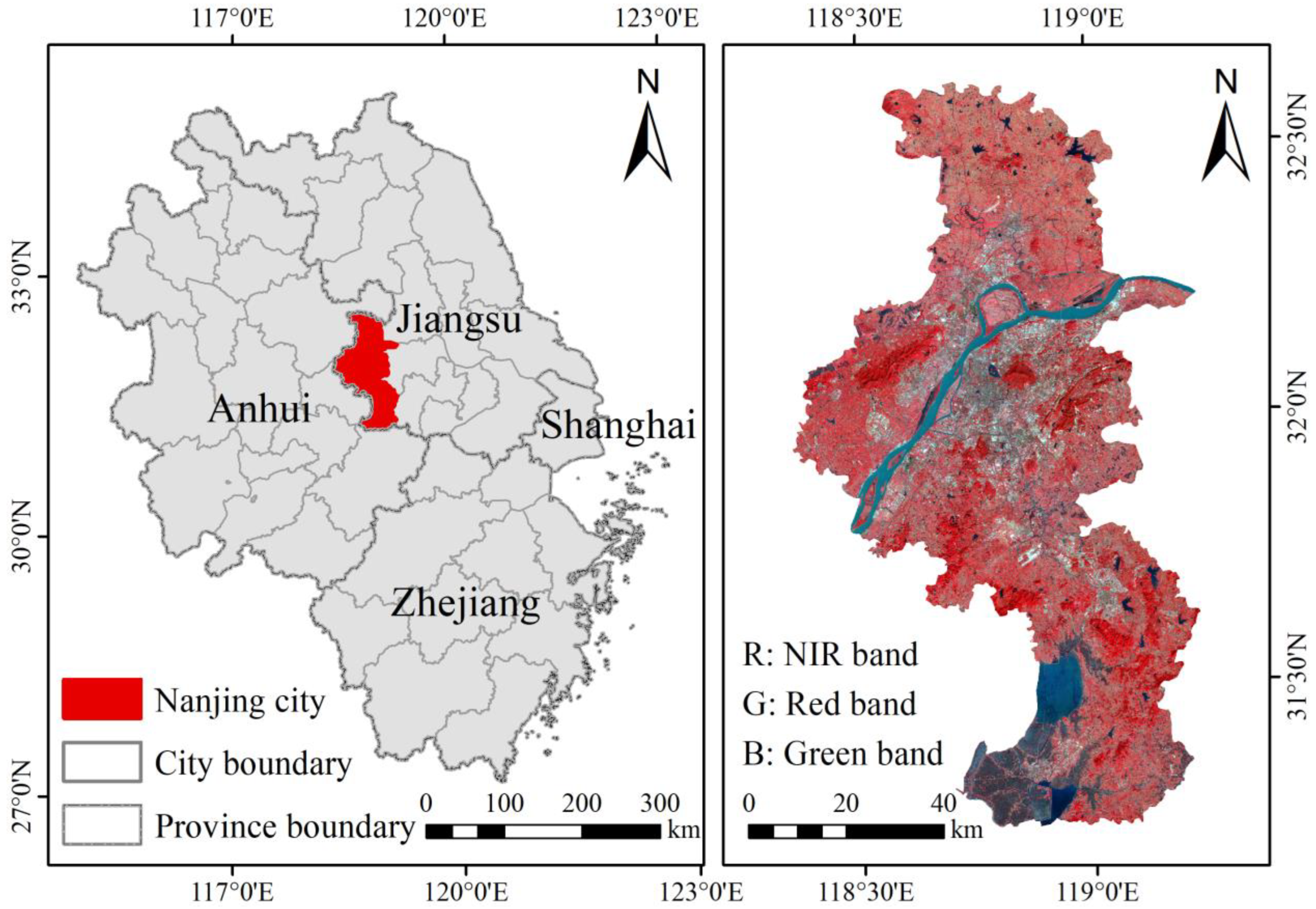
Nanjing City is situated between 31°14′ and 32°37′N and 118°22′ and 119°14′E in eastern China, in the middle of the Yangtze River’s downstream section (Figure 1). As of 2021, Nanjing had 11 districts with a total area of 6587.02 km2, a permanent population of 9,423,400 people, including 8,188,900 people in urban areas, with an urbanization rate of 86.9%, and a gross domestic product (GDP) of 231.37 billion USD. A northern subtropical humid climate with four distinct seasons and copious rainfall characterizes Nanjing. With 117 rainy days on average year and 1294.4 mm of rainfall, the average annual temperature is 17.1 °C [37].
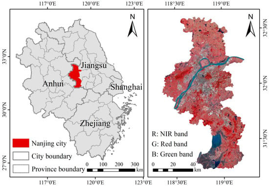
Figure 1.
Location of Nanjing City and false-color composite of Landsat 8 images. Note: R: NIR band, G: Red band, and B: Greed represent the near-infrared, red, and green bands of Landsat 8 images, respectively.
As one of China’s hottest cities, Nanjing’s urban development has undergone substantial change over the past 30 years. According to Yang and Huang [38] annual China land cover dataset (CLCD), which was created using Landsat data, Nanjing’s impervious surface area expanded from 444.27 km2 in 1990 to 1371.95 km2 in 2020, more than tripling in size over previous three decades. In addition, the permanent population of Nanjing is increasing rapidly, from 6,148,500 in 2000 to 9,423,400 in 2021. Rapid urbanization with the increase in population and impervious surfaces has significantly changed the underlying surface types in Nanjing, which result in LST changes and intensification of the UHI effect [26].
2.2. Datasets
2.2.1. Landsat Data
We collected all available Landsat 5 and Landsat 8 L1TP level surface reflectance (SR) data for the summers (June to September) of 1990–2020 over the study area from the Google Earth Engine (GEE) and used median composites for the synthetic annual images. GEE is an online remote sensing cloud platform that allows users to perform remote sensing big data computation and analysis quickly and efficiently without the need for computational resources [39,40,41]. These data contained a cloud, shadow, water, and snow mask created using a C Function of Mask (CFMASK) algorithm and were atmospherically adjusted using Land Surface Reflectance Code [42] and per-pixel saturation mask. All available images were retrieved, and cloud coverage information, including cloud shadowing, was removed from the images based on the quality assessment bands provided by the USGS through GEE. In addition, Landsat 5 and Landsat 8 data were considered consistent and inter-calibrated [39], and all TIR bands were resampled using cubic convolution to 30 m [43].
2.2.2. LULC and Its Driving Factors
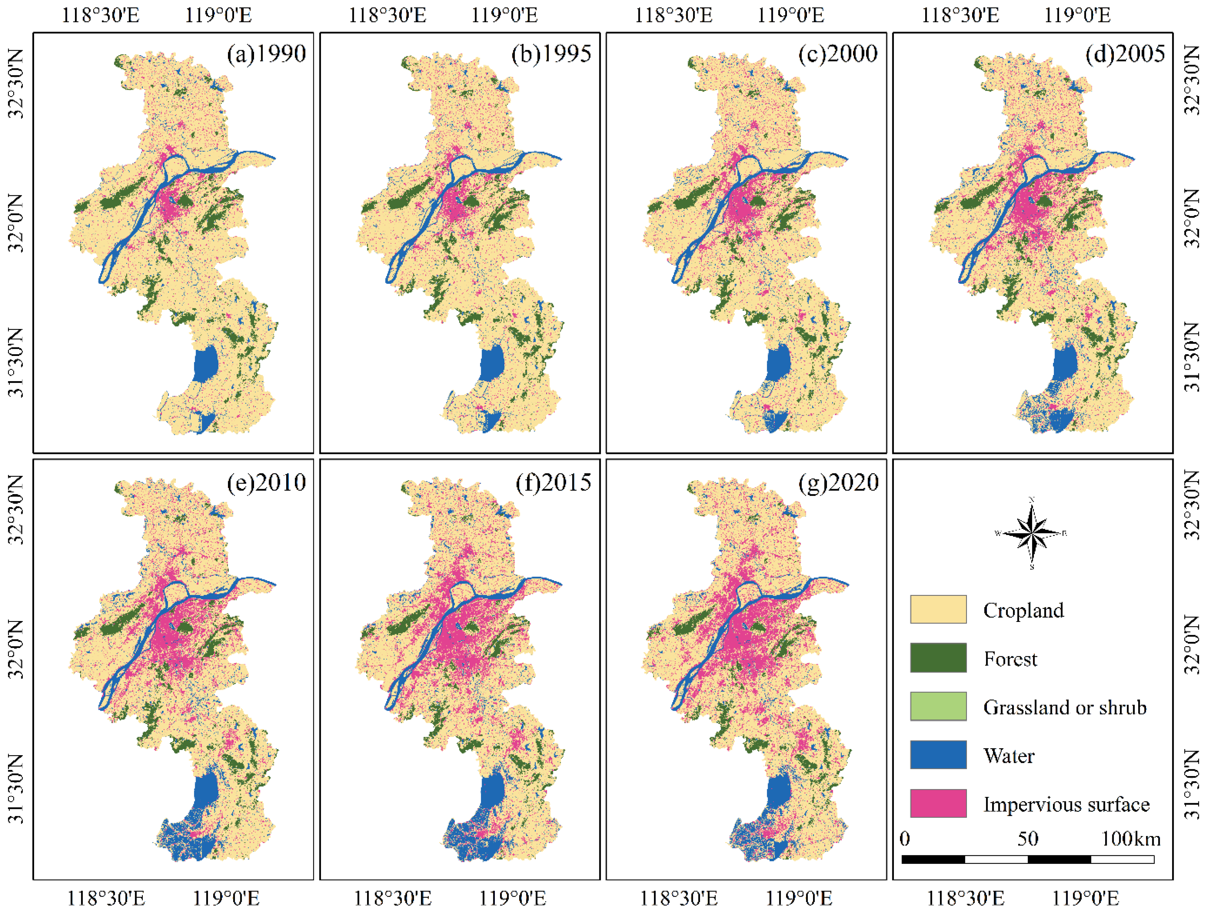
The LULC data for Nanjing from 1990 to 2020 (five-year interval) were obtained from the CLCD dataset [38], which provides the annual LULC distribution for Nanjing from 1900 to 2020. Based on the actual land use conditions in Nanjing, the CLCD was divided into five types: cropland, forest, grassland or shrub, water, and impervious surface (Figure 2). Previous studies have confirmed that LULC changes are affected by socioeconomic development and climate change [36,44]. Therefore, we collected 18 potential driving factors that affect LULC changes in our study area, including GDP, population density, soil type, digital elevation model (DEM), slope, temperature, precipitation, night-time light [45], and vector data for residents, railroads, and various roads (Table S1). All driving factor data were transformed into raster data in the same projection coordinate system (UTM Zone 50N) at a spatial resolution of 30 m.

Figure 2.
Historic LULC (land use and land cover) data in 1990−2020 (five-year interval) for Nanjing City.
The future temperature, precipitation [46], GDP [47], and population density [48] data used to simulate future LULC changes were derived from three typical climate change scenarios from the Coupled Model Intercomparison Project (CMIP) [49,50,51,52], i.e., SSP126, SSP245, and SSP585. Among these, SSP126 is an integrated SSP1 and RCP2.6 scenario that shows a green way forward for low levels of greenhouse gas (GHG) emissions and sustainable socioeconomic growth. An intermediate pathway with a middle level of socioeconomic and technical growth and a medium level of GHG emissions is SSP245—an integrated scenario of SSP2 and RCP4.5. SSP585 indicates a very high degree of fossil fuel consumption and high GHG emissions from a high-end forcing pathway and is a combined scenario of SSP5 and RCP5.8 [53,54].
3. Methodology
3.1. LST Derivation
3.1.1. Calculation of Proportion of Vegetation
The proportion of vegetation (PV) is commonly derived using the NDVI, which can be given as follows:
where NDVI represents the original value of NDVI, NDVIMin, and NDVIMax are the minimum and maximum values of NDVI in an image, respectively [55].
3.1.2. Calculation of Surface Emissivity
The surface-specific emissivity is calculated by the equation as follows [56]:
where ε is the surface-specific emissivity.
3.1.3. Calculation of LST
The thermal infrared radiation reaching the satellite sensor is affected by atmospheric radiation, and the atmospheric influence on the surface thermal radiation must be eliminated from the total thermal radiation. The LST can then be calculated using the Plank function, which is expressed as [57]:
where λ is the central wavelength of the thermal infrared band, corresponding to 10.40 μm for Landsat 5 and 11.45 μm for Landsat 8; ρ is the constant of 1.438 × 10⁻²; and B(Ts) is the thermal radiation of the blackbody when the temperature is Ts, which can be calculated by the following formula:
where K1 = 607.76 W/(m2·sr·μm) and K2 = 1260.56 K for Landsat 5 TM images; K1 = 774.89 W/(m2·sr·μm) and K2 = 1321.08 K for Landsat 8 OLI/TIRS images; and ρT is the thermal infrared spectrum of Landsat.
3.2. Acquisition of Potential Driving Factors of LST
Surface temperature is influenced by a combination of various drivers. We calculated ten potential drivers based on Landsat data and LULC data to explore their effects on LST, including NDVI, NDBI, soil-adjusted vegetation index (SAVI), modified normalized difference water index (MNDWI), tasseled cap (TC) greenness (TCG) and TC wetness (TCW) components after TC transformation, as well as impervious surface, forest, water body, and cropland distribution density (Table S2). NDVI is the most commonly used vegetation index for monitoring vegetation growth conditions and health [58,59,60]. The NDBI is a widely used indicator for extracting built-up areas [61,62]. The MNDWI proposed by Xu [63] is a commonly used water index that can effectively suppress signals from building surfaces and accurately distinguish building surfaces from water pixels [64]. It is widely used in surface water mapping, land use/cover change analysis, and ecological studies [65,66,67]. In sparsely vegetated areas with exposed soil, reflectance values in the red and near-infrared bands are affected, which influences the NDVI estimation results [68]. To eliminate the effect of soil background, Huete [69] proposed the SAVI, which adds a soil adjustment factor L to NDVI. In this study, we set L as 0.5 to fit most land covers [69]. TCG and TCW are the greenness and wetness parameters of TC transformation [70,71], respectively.
Meng et al. [26] proposed a method for determining the distribution density of impervious surfaces in order to assess the degree of dispersion of urban impervious surfaces and to guarantee the integrity of urban subsurface types. The degree and density of the impervious surface distribution within a specific radius centered on the pixel are referred to as the pixel’s ISDD [72]. The density inside the radius is represented by the average value. The weight, which may be used to quantify the degree of dispersion of buildings within the radius, increases as the impervious surface image element approaches the center. The calculation formula is as follows:
where s is the central pixel; r is the calculation radius; Bsi is the value of ith pixel within radius r (impervious surface pixel = 1; permeable surface = 0); Di is the distance between ith pixel and the central pixel; and the summation refers to all pixels within a circle with radius r. We extended the formula to calculate the distribution density of croplands, forests, and water. It is notable that because of the small area of the grassland or shrubland type, this land type was not included in the discussion.
3.3. Simulation of the Future LULC Data Using the PLUS Model
The PLUS model is able to simulate future LULC in combination with future predictor variables dynamically and thus is particularly suitable for this study [36]. The land use demands for the three future climate change scenarios were obtained based on historical land use data [73] and Markov chain methods [36,74,75]. We compared the actual 2020 LULC data with the 2020 LULC data predicted by the PLUS model using the 2010 and 2015 LULC data as well as 18 driving factors that impact LULC in order to evaluate the model’s accuracy. The PLUS model was used to simulate LULC under various climate change scenarios if the simulation results’ accuracy was found to be adequate [34,35].
3.4. Projection of Future LST
Previous studies have shown that LST has a robust relationship with land cover indices [4,20,76,77,78], including NDVI, NDBI, SAVI, MNDWI, TCG, TCW, ISDD, cropland distribution density (CDD), forest distribution density (FDD), and water distribution density (WDD). The partial least squares regression (PLSR) method was used to evaluate the regression relationship between LST and ten potential factors in 2020. This methodology is more succinct and statistically reliable than principal component regression because it combines the advantages of principal component analysis with multiple regression [79,80]. Moreover, PLSR is well suited to this case because it can effectively avoid overfitting problems due to the high linear correlation between variables [81]. The regression equation (R2 = 0.735) for LST and the ten driving factors are as follows:
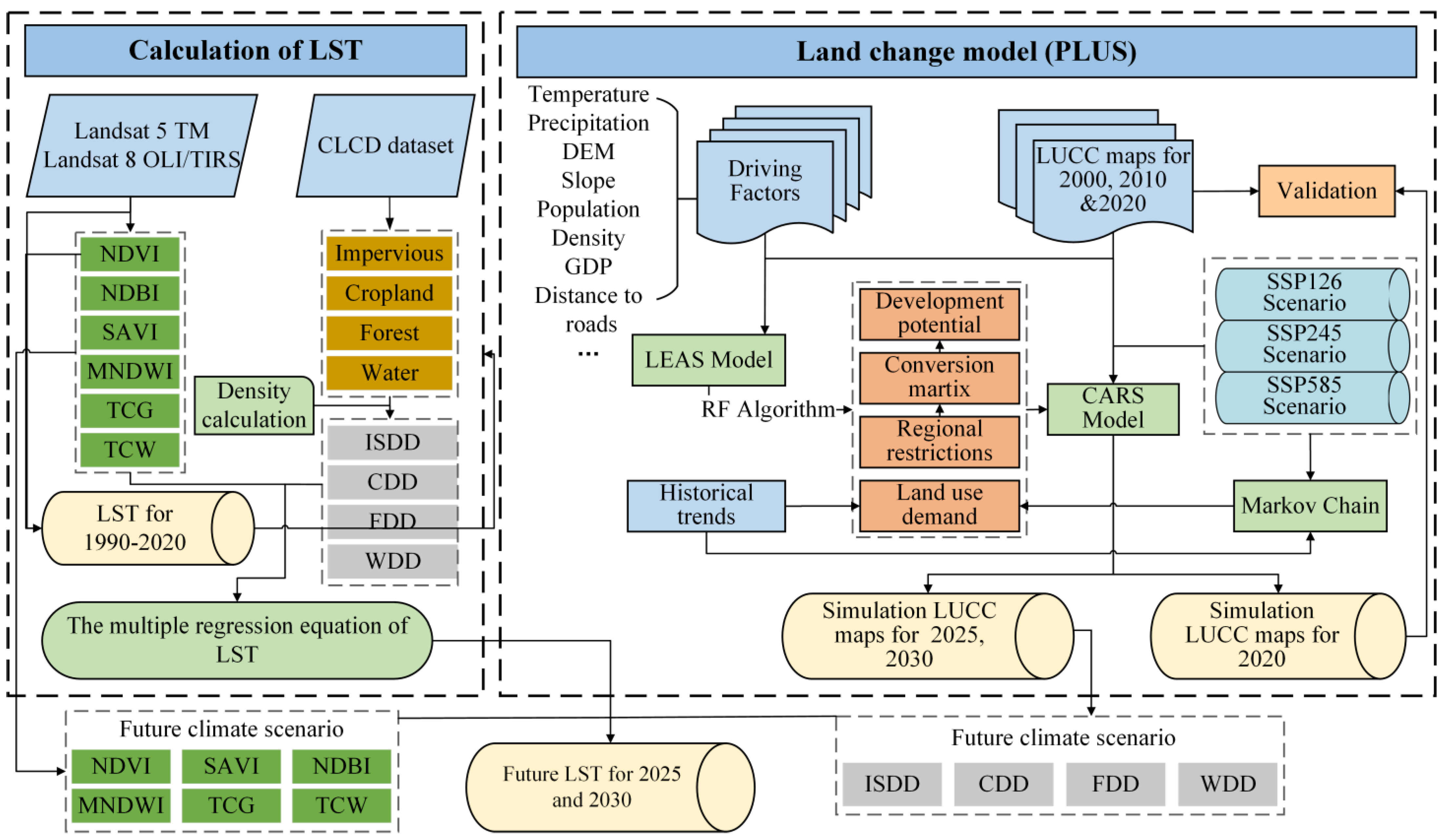
Using an approach that accounts for both structural and local differences in these indices, future coverage indices were simulated [20]. Figure 3 illustrates the simulation workflow for NDVI as an example. The local component shows the local index variations brought on by LULC changes, while the structural component shows the overall shift in the coverage indices over time. After a comprehensive analysis of NDVI and LULC changes over the past 30 years, the process described above was used to simulate NDVI under the future SSP126 scenario. The NDBI, SAVI, MNDWI, TCG, and TCW were simulated using a similar method. The future ISDD, CDD, FDD, and WDD were calculated from the LULC data simulated by the PLUS model using Equation (5). Finally, we used Equation (6) to project future LST for 2025 and 2030. The workflow of the future land use simulation and LST projection is illustrated in Figure 4.
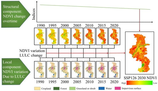
Figure 3.
The workflow of NDVI (normalized difference vegetation index) simulation in 2030 under future SSP126 scenarios.
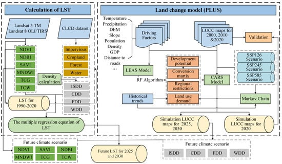
Figure 4.
The workflow of land use simulation and land surface temperature prediction under future climate change scenarios.
3.5. UHI Intensity Calculation and Classification
We utilized the same standard to assess the UHI intensity for multiple periods since it is inappropriate to directly compare the absolute temperature readings when reporting the UHI intensity at different times. That is, we defined the UHI intensity (∆T) as the mean LST difference between impervious and non-impervious surfaces:
where TImpervious and TNon-impervious are the mean LST of the impervious surface and the non-impervious surface, respectively. The UHI intensity levels are listed in Table 1.

Table 1.
Definition of UHI (urban heat island) intensity levels.
4. Results
4.1. Spatiotemporal Patterns of LST during 1990–2020
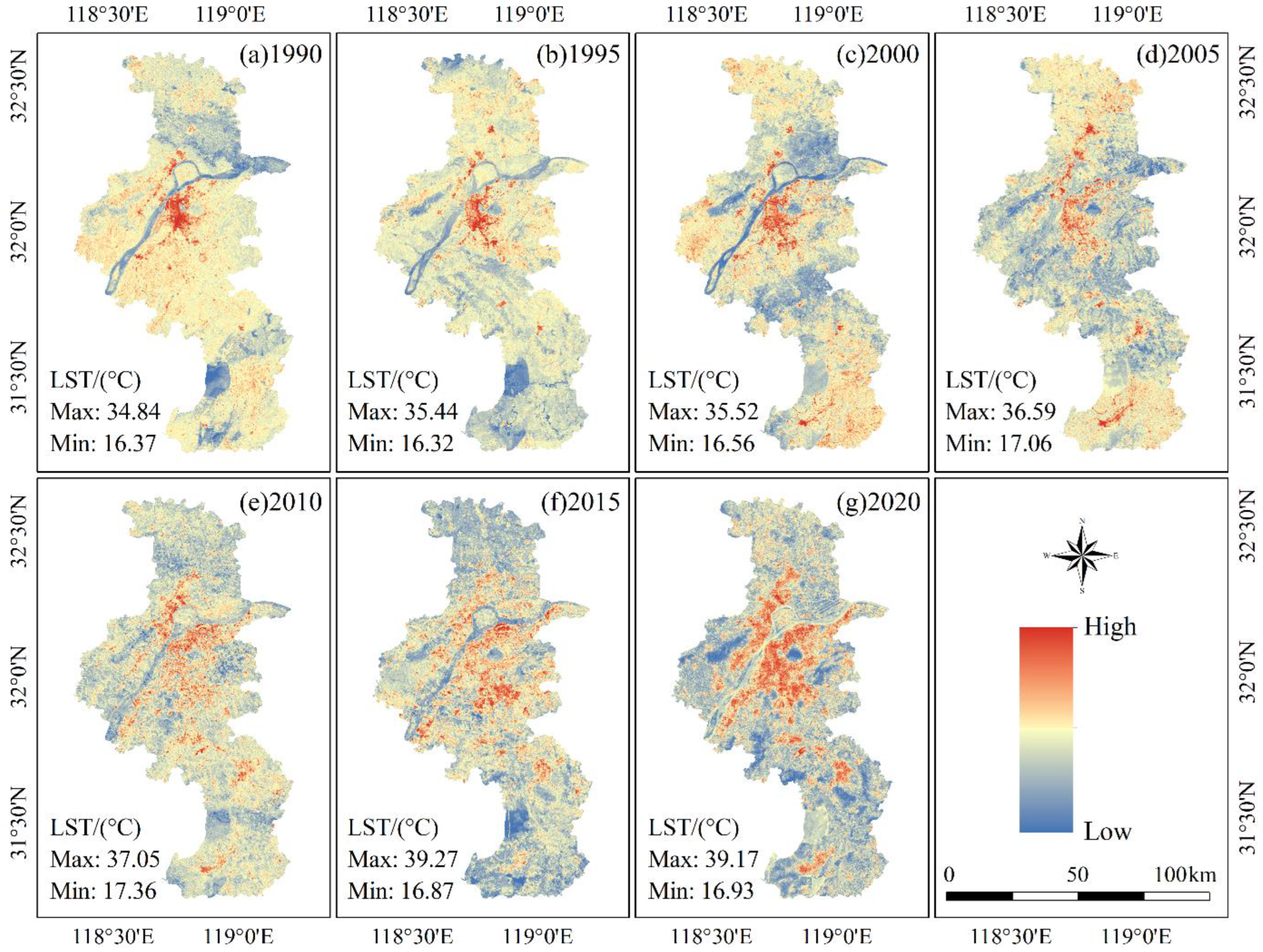
Figure 5 illustrates the spatial distribution pattern of LST in the summer (June to September) in Nanjing from 1990 to 2020, where the high surface temperature areas are mainly concentrated in the impervious surface area and have been expanding since 1990. The maximum value of LST showed a continuous increase from 34.84 °C in 1990 to 39.17 °C in 2020 and peaked in 2015 (39.27 °C). The minimum value of LST was consistent with the maximum value trend, i.e., its value continuously increased. LST varied greatly among the land use types (Table 2), with impervious surfaces showing the highest LST, followed by cropland and forest, and water having the smallest LST. Specifically, from 1990 to 2020, impervious surfaces showed the largest increase (2.24 °C) in mean LST, whereas forests had the smallest increase (1.38 °C) in mean LST, which reflects the effect of land use and coverage index changes on LST over the past three decades. The VNP21A1D: Day Land Surface Temperature and Emissivity Daily 1 km product from the GEE [82] was used to validate the 2020 LST results, and the results showed a consistency of 86.37%, which indicated the reliability of the LST extracted for this study. In addition, Figure 5 clearly shows that the high LST areas of Nanjing in 1990 were distributed from the initial areas mainly in the Qinhuai, Gulou, and Xuanwu districts around the city center to a large number of high LST areas in almost all administrative districts of Nanjing in 2020. In general, the development pattern of the high LST region has maintained a similar spatial and temporal pattern to the land use changes in Nanjing over the past three decades (Figure 2).
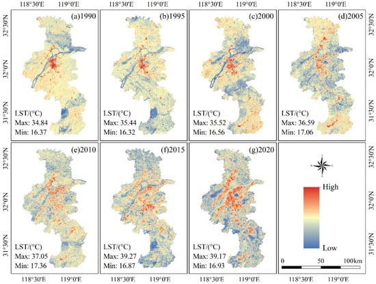
Figure 5.
Spatial patterns of LST (land surface temperature) in Nanjing from 1990 to 2020.

Table 2.
Statistics of mean LST (land surface temperature) for different land use types in Nanjing from 1990 to 2020.
4.2. Simulation of LULC Data in Nanjing for 2025 and 2030
We projected Nanjing’s land use patterns for 2025 and 2030 under several climate change scenarios using the PLUS model (Figure 6). Significant changes in land use were anticipated compared to 2020, and the pattern of land use varied greatly across the various scenarios (Table 3). Specifically, by 2030 under the SSP126 scenario, arable land and grassland or shrubs will experience varying degrees of decrease, while forests will be effectively protected, with a predicted increase of 13.44 km2 and 0.20%. The impervious surface area will have a small increase of 63.71 km2 or 0.97%. In addition, the water remained stable.
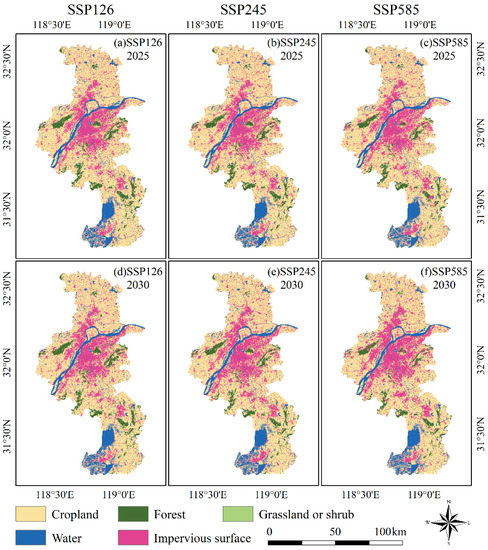
Figure 6.
Simulation of LULC (land use and land cover) in Nanjing under different climate change scenarios.

Table 3.
Statistics of land use changes in Nanjing from 2020 to 2030 under different climate change scenarios.
Under the SSP245 scenario, the cropland area is further decreased from 4139.20 km2 in 2020 to 4011.60 km2 in 2030, a total decrease of 127.60 km2 and a decrease of 1.93% in proportion. The forest is not effectively protected, and the area will decrease by 39.44 km2 by 2030. The impervious surface area has a higher increase than the SSP126 scenario and is expected to increase by 168.29 km2, reaching 23.34% of the total area by 2030. The changes in grassland or shrubs and water were similar to those in the SSP126 scenario. Notably, under the SSP585 scenario, the cropland area decreased significantly (185.92 km2) from 62.73% in 2020 to 59.91% in 2030. The forest will be destroyed, with the area decreasing to 100.24 km2 by 2030. In contrast, the impervious surface expands significantly, increasing from 1371.95 km2 in 2020 to 1659.03 km2 in 2030, an increase of 4.35%. Such a substantial land use change will lead to future changes in the coverage indices and land use distribution density and further result in a continued general increase in LST.
4.3. Simulation of Coverage Indices in Nanjing for 2025 and 2030
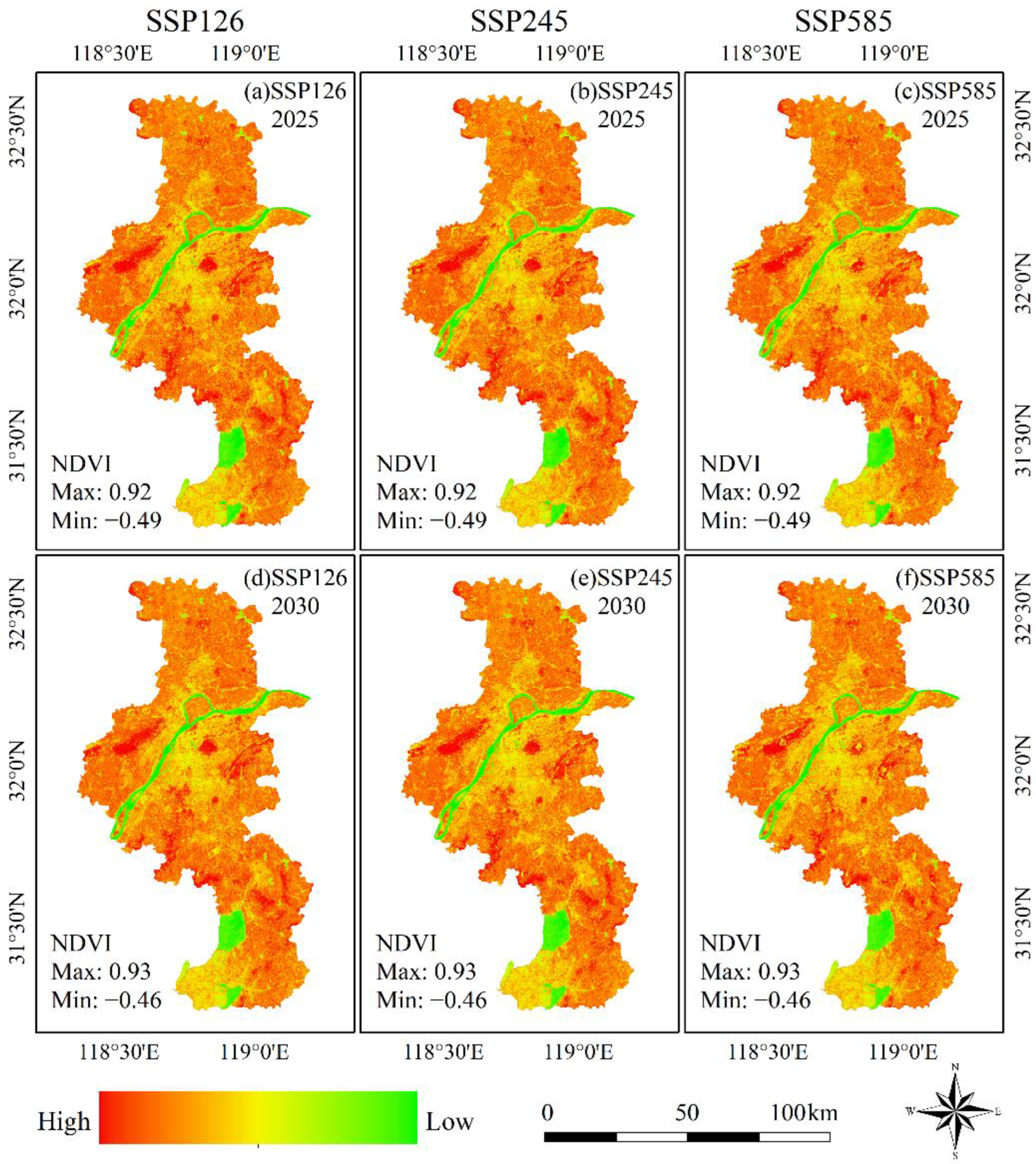
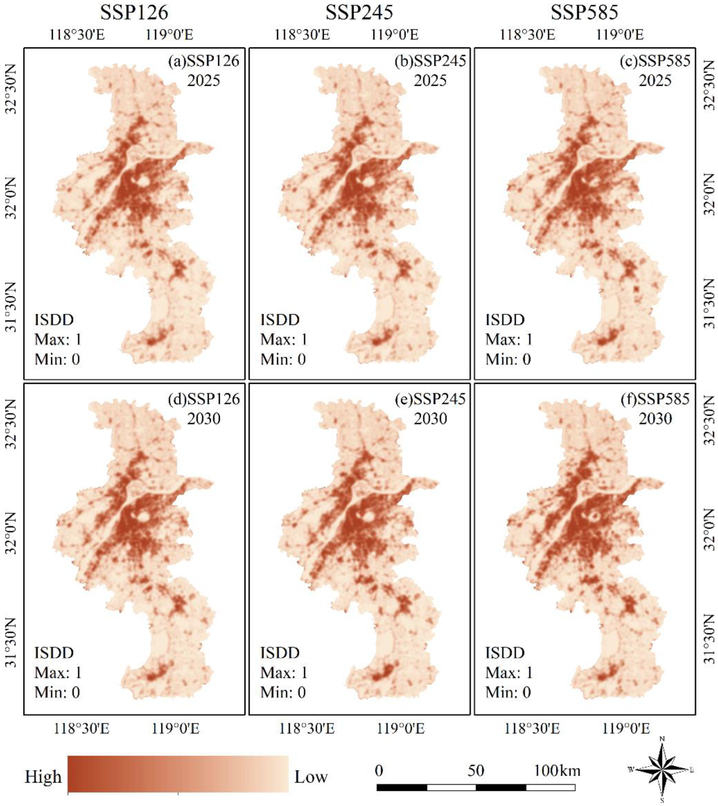
The simulated future LULC data of Nanjing combined with the workflow in Figure 3 were used to simulate the land coverage indicators under different future climate change scenarios, including NDVI, NDBI, SAVI, MNDWI, TCG, TCW, ISDD, CDD, FDD, and WDD, which were calculated using Equation (5). Figure 7 and Figure 8 illustrate the simulation results for NDVI and ISDD, respectively, and the other coverage indices are provided in Figures S1–S8. The coverage indices were very similar under different climate scenarios; however, a visual interpretation revealed that the main differences occurred in areas of land use change, which was consistent with our expectation that land use change would lead to changes in coverage indices.
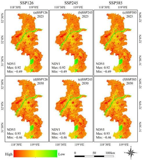
Figure 7.
Simulation of NDVI (normalized difference vegetation index) in Nanjing under different climate change scenarios.

Figure 8.
Simulation of ISDD (impervious surface distribution density) in Nanjing under different climate change scenarios.
Furthermore, there were notable differences in the coverage indices under different scenarios compared with 2020. For example, the NDVI increased slightly under the SSP126 scenario (Figure 7a,d), whereas it decreased relatively more under the SSP585 scenario (Figure 7c,f). The ISDD increased slightly under the SSP126 scenario (Figure 8a,d) and decreased significantly under the SSP585 scenario (Figure 8c,f). Similar trends in NDVI and ISDD, as described above, were observed for other coverage indices, except for water bodies. As expected, the dramatic land use and coverage index changes predict that the LST of Nanjing will change significantly in 2025 and 2030.
4.4. Predicting LST of Nanjing in 2025 and 2030
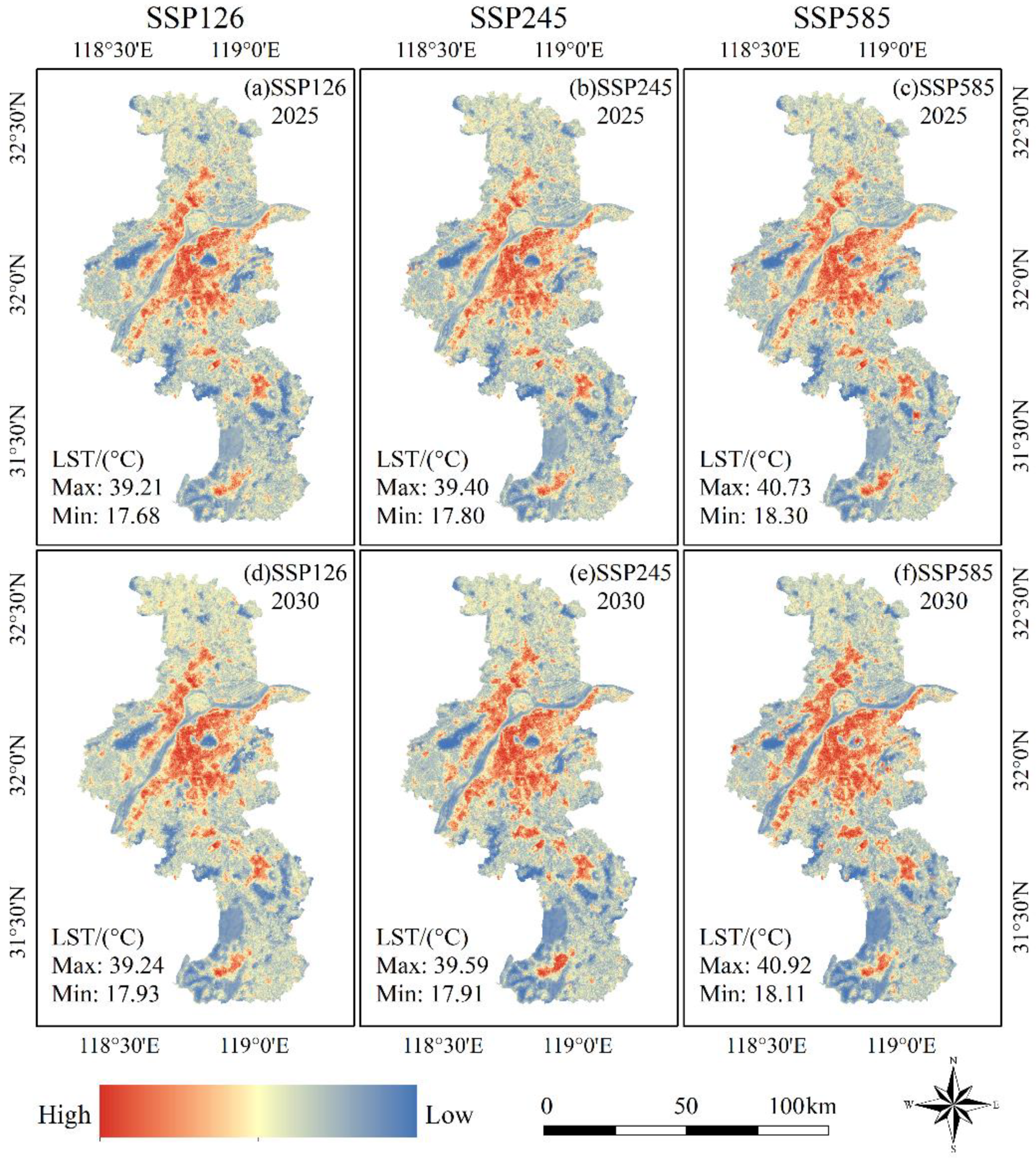
We used the simulated ten land coverage indicators as input layers, combined with Equation (6), to obtain the LST of Nanjing for 2025 and 2030 under different future climate scenarios (Figure 9). The results show that the LST of Nanjing under the three scenarios shows different degrees of increase during 2020–2030. According to multiple scenarios, Table 4 shows the mean LST for Nanjing in 2025 and 2030. It is clear that the mean LST for each kind of land use is greater under the SSP585 scenario than it is under the SSP126 scenario. By 2030, impervious surfaces will have the highest mean LST (28.94 °C), followed by cropland (26.23 °C) and forest (25.18 °C), whereas water bodies have the lowest mean LST (24.02 °C), which is also consistent with the mean LST pattern of different land use types over the past three decades (Table 2).
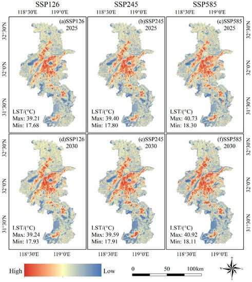
Figure 9.
The LST (land surface temperature) projections for Nanjing in 2025 and 2030 under different climate change scenarios.

Table 4.
Statistics of mean LST (land surface temperature) of Nanjing in 2025 and 2030 under different climate change scenarios.
Compared with 2020, except for forest, the mean LST increased slightly for the other three land use types in 2030 under the SSP126 scenario. The mean LST of the forest decreased from 24.39 °C in 2020 to 24.25 °C in 2030. Under the SSP245 scenario, the mean LST of each land use type will increase faster by 2030. Among the five land use types, the mean LST of impervious surfaces increased by 0.52 °C. Under the SSP585 scenario, a relatively large increase was observed in the mean LST for each land use type. By 2030, the mean LST of impervious surfaces will approach 29 °C, and the mean LST of water bodies will exceed 24 °C. The mean LST of impervious surface, cropland, forest, and water bodies will increase by 1.37, 1.12, 0.79, and 0.61 °C, respectively.
To further explore the spatiotemporal characteristics of LST in 2025 and 2030 under different scenarios, we calculated the difference between the LST maps in 2025 and 2030 and the LST map in 2020, as illustrated in Figure 10. Significant differences in the distribution of the Nanjing LST differences under different scenarios can be observed (Table 5). Under the SSP126 scenario, only 1.42% of the study area will experience a decrease in LST by 2025, while there are almost no areas where the LST increases by more than 3 °C. By 2030, the LST decrease area will increase to 1.72%, and 0.05% of the areas will have an LST increase greater than 3 °C. Under the SSP245 scenario, 90.77% of the study area will have an increase in LST of 0–1 °C by 2025, and 8.73% of the area will have an increase in LST of more than 1 °C. By 2030, 71.93% of the study area will have a 0–1 °C increase in LST, and 27.56% of the area will have an LST increase of more than 1 °C. In contrast, under the SSP585 scenario, only 0.20% of the study area will experience a decrease in LST by 2025, which will further decrease to 0.11% by 2030. The area with an LST increase of more than 1 °C also increases from 20.35% in 2025 to 45.79% in 2030, and the area with an LST increase of more than 3 °C reaches 3.97%. Overall, there were significant differences in future LST changes under different climate scenarios, and the different climate scenario patterns leading to different LST changes depend on the developmental pathway that is taken.
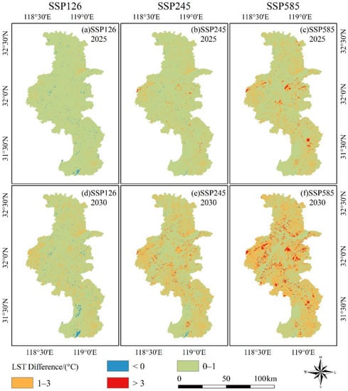
Figure 10.
Difference maps of LST (land surface temperature) under different climate change scenarios compared to 2020.

Table 5.
Statistics of the LST (land surface temperature) difference under different climate change scenarios.
4.5. Spatiotemporal Distribution of UHI Intensity Levels
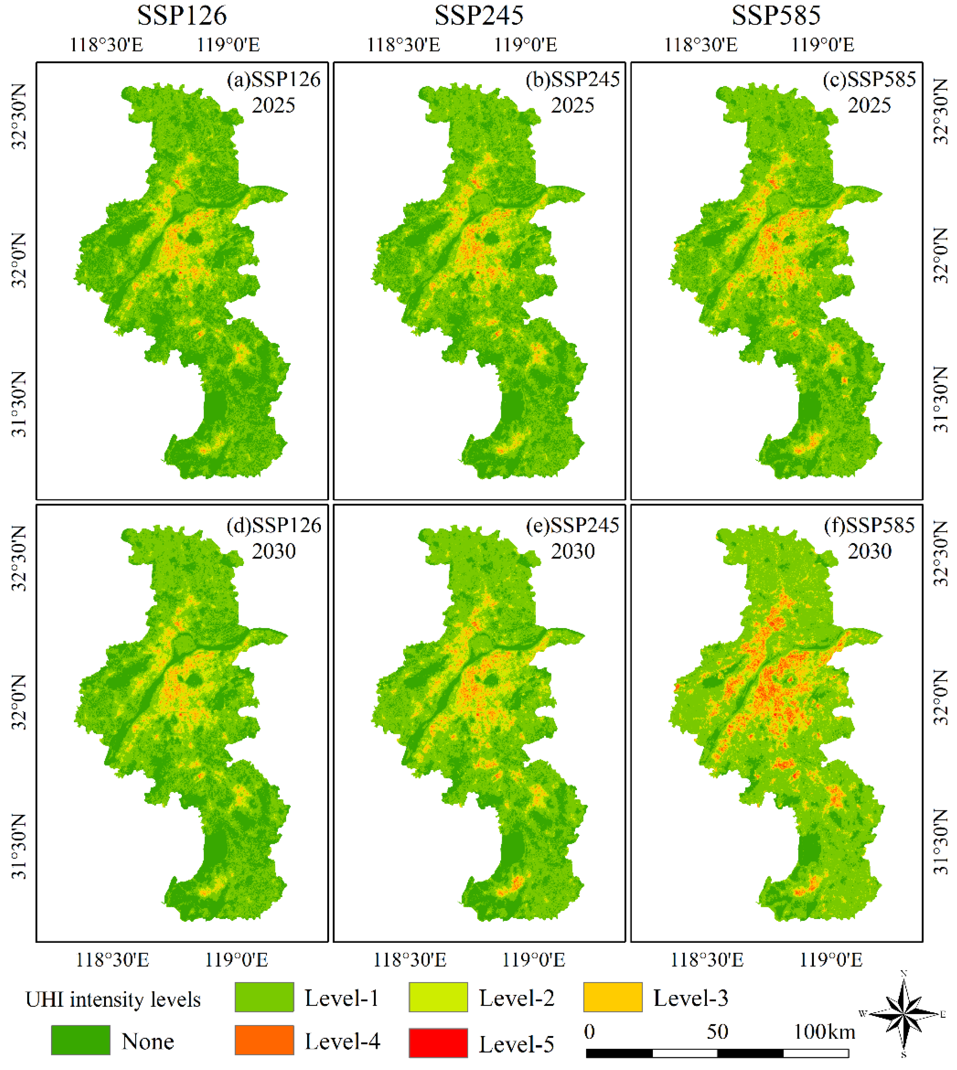
Based on Equation (7) and Table 1, the distribution of the UHI intensity levels in 2025 and 2030 for Nanjing under various scenarios is shown in Figure 11. We conducted a statistical study of the UHI intensity in 2025 and 2030 under several scenarios in order to more accurately assess the regional and temporal evolution of the UHI intensity (Table 6). Under the SSP126 scenario, the UHI effect will be observed for 57.78% of the study area by 2025, with this percentage increasing to 63.95% by 2030. Nonetheless, the percentage of areas with high UHI intensity levels (Level-4 and Level-5) decreases under this scenario, with Level-4 and Level-5 UHI intensities decreasing from 0.41% and 0.02% in 2025 to 0.32% and 0.01% in 2030, respectively. This indicates that the high UHI effect in Nanjing is mitigated under the SSP126 scenario and is further reduced as this scenario continues.
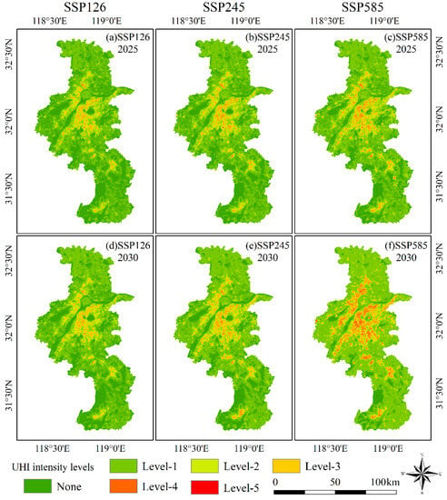
Figure 11.
UHI (urban heat island intensity) levels of Nanjing in 2025 and 2030 under different climate change scenarios.

Table 6.
Statistics of UHI (urban heat island intensity) intensity levels of Nanjing in 2025 and 2030 under different climate change scenarios.
Under the SSP245 scenario, the UHI effect in Nanjing continues to increase, with the affected area increasing from 65.06% in 2025 to 73.49% in 2030. The percentage of areas with a UHI intensity level of 3 or higher will reach 7.05% by 2030. The UHI effect was the strongest in Nanjing under the SSP585 scenario. By 2030, only 10.38% of the study area will have no observed UHI effect. Levels 3, 4, and 5 of UHI intensity in 2030 will be 10.31%, 3.74%, and 0.14%, respectively. The spatial distribution of high-level UHI intensity areas (Figure 11) and the distribution of high ISDD highly overlap (Figure 8), which is consistent with the previous assumption that the higher the distribution density of impervious surfaces, the stronger the UHI effect. Overall, the high-level UHI effect in Nanjing will slightly mitigate over time under the SSP126 scenario, whereas the UHI effect in Nanjing will continue to increase under the SSP245 and SSP585 scenarios, especially in the SSP585 scenario.
5. Discussion
Future LULC simulations may be used to reliably forecast future LST patterns based on the assumption that land use change impacts would have an impact on LST. The PLUS model can combine future predictor variables with Markov chains to accurately simulate changes in land use distribution (the overall accuracy is approximately 95%) under the constraints of future land use demand and development probabilities of different land use types. The PLUS model retains the benefits of the cellular automata model’s adaptive inertial competition and roulette wheel competition mechanisms [34,36]. Future land-coverage indicators must be correctly predicted in order to forecast future LST. The temporal changes in the indices are divided into structural and local components in our technique for forecasting the coverage indices [20], which can accurately identify the changes in the coverage indices due to land use changes. Consequently, the distribution pattern of the future coverage index can be determined in a more refined manner. Based on the calculation method of impervious surface distribution density proposed by Meng et al. [26], we extended it to the distribution density calculation of other land use types. Using the above two methods, we generated reasonable land coverage indicators NDVI, NDBI, MNDWI, SAVI, TCG, TCW, ISDD, CDD, FDD, and WDD and successfully used them to predict the LST of Nanjing for 2025 and 2030 (Figure 9).
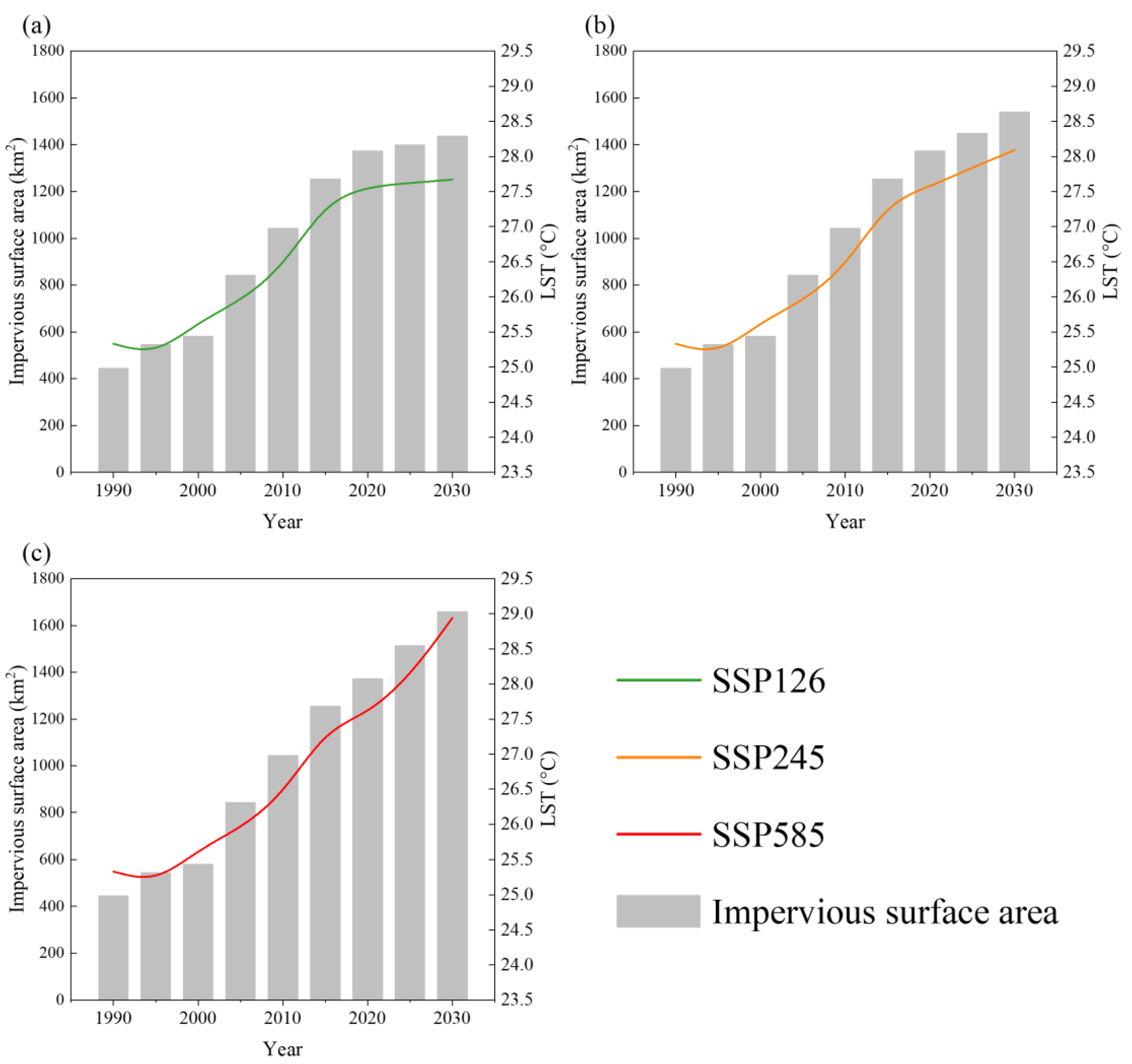
Our results show that LST in Nanjing continuously increases from the past to the future (for all three climate scenarios). We observed that the increase in LST in Nanjing was consistent with the increase in the impervious surface area (Figure 12). Specifically, under the SSP126 scenario, the trend of increasing LST slows as urban sprawl is effectively controlled, and the increase in urban impervious surface area slows down (Figure 12a). Under the SSP245 scenario, the urban impervious surface area maintained a high growth rate, and the LST increased rapidly with an increase in impervious surface area (Figure 12b). Not surprisingly, the rate of increase in LST reached a maximum because of the sharp increase in impervious surface area under the SSP585 scenario (Figure 12c). This is consistent with previous studies that showed a strong linear relationship between impervious surface area and LST, where LST increased with an increase in impervious surface area [4,26,83]. Rapid urbanization concentrates a sizable population in a little amount of time in economically developed cities such as Nanjing. As a result, to accommodate the city’s growth, there must be extensive urban building, a thriving real estate market, and a high demand for industrial property. The consequence of rapid urban expansion is an increasing impervious surface area, which leads to changes in the underlying urban surface types and land surface environment [20]. The large absorption capacity and high radiation temperature of the impervious surface might lead to an increase in sensible heat and an increase in LST [84].
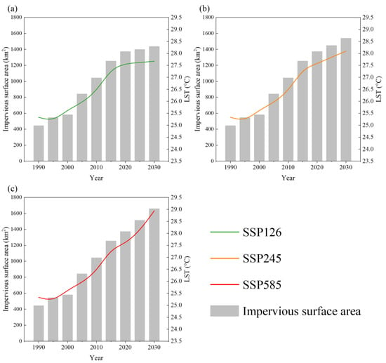
Figure 12.
Relationship between LST (land surface temperature) and impervious surface area under different climate change scenarios. (a) SSP126 scenario; (b) SSP245 scenario; (c) SSP585 scenario.
The poor distribution of the urban thermal environment will result in the UHI effect that would challenge the sustainability and livability of cities. In this study, the future LST projections for the mean temperature of impervious surfaces were significantly higher than that of other land use types (Table 4), which was the main reason for the intensified UHI effect. Previous studies have found that vegetation and water bodies effectively reduce the local thermal environment in cities [20,85]. Therefore, considering vegetation and water zoning in planning and design within cities will help regulate the thermal environment, which may be the most effective solution to reduce the UHI effect within cities [33]. In some sense, increasing the proportion of urban land use types such as forests, grasslands, shrubs, and water bodies can reduce the LST and mitigate the UHI effect to some extent. Furthermore, reducing the impervious surface density also mitigates the UHI effect [26], which is due to the fact that when the impervious surface patch gap becomes larger, previously accumulated heat could be released from the surface, hence reducing the LST [86]. Therefore, in order to mitigate the UHI, the primary emphasis of urban design efforts should be on changing the material composition of the land surface [87], such as reducing the distribution area of impervious surfaces. In addition, the distance between the city and the river, the height of buildings, and the shape of green spaces may have a significant impact on the distribution of LST, and this is an important element of future urban planning to deal with the UHI effect [87]. The type of urban development is also a factor that influences the LST and UHI. In general, the infill development pattern has higher urban LST than that of the leapfrog development pattern. This is due to the surrounding high LST land use types (such as built-up areas), which create greater urban LST surrounding the infill-developed urban regions. Leapfrog urban areas, on the other hand, are bordered by other land use categories with a lower LST, including agricultural land. Additionally, effective planning techniques such as urban design that include an adequate percentage of public spaces, such as parks and lakes, aid in lowering LST [33]. It is worth mentioning that for the same population capacity, we should try to build high-rise buildings in order to expand the shaded area, improve local ventilation and use the protected land for green space and water bodies. Overall, the projected future LST distribution pattern provides an insight that plays an irreplaceable role of vegetation in mitigating UHI should not be ignored in urban land resource reallocation and that rational urban layout [88], good LULC structure, and vegetation “greening strategies” are effective measures to reduce LST and mitigate urban UHI effect.
Notably, there still exist some limitations in this study. First, the LULC data used in this study were derived from the CLCD dataset. Although this dataset was proven to have a high overall accuracy (79.31%) [38], however, the accuracy of future LULC and LST predictions is based on the existing LULC. Therefore, LULC data with high classification accuracy could contribute to reducing the uncertainties of future LULC and LST predictions [20,34,36]. Second, we only considered 18 driving factors affecting changes in LULC and did not consider more potential driving factors affecting changes in LULC, such as economic factors, policy planning, etc. In the future, we will consider more potential factors to improve the study framework [36]. Finally, there are some uncertainties in the regression relationship between LST and driving factors [20,76]. We will focus on improving the accuracy of the regression relationship between LST and driving factors in future research to obtain better LST prediction results. Despite the above limitations, this study proposed a method for predicting future LST that considers land use change effects and provides distribution patterns for land use and LST in Nanjing under different climate change scenarios. Clearly, the research framework proposed in this study is also applicable to future LST projections and UHI simulations for other mega-cities in China or around the world [4,15,76]. Indeed, this is also the ambition and challenge of our future work.
6. Conclusions
In this study, we retrieved the 1990–2020 LST and associated coverage indices for Nanjing using Landsat imagery data and explored their spatiotemporal dynamics with LULC in the study area. We also simulated the LULC of Nanjing for 2025 and 2030 under different climate scenarios using the PLUS model and LULC driving factors and simulated the corresponding land coverage indicators. By establishing a regression relationship between LST and land coverage indicators by the PLSR method, we successfully predicted the LST of Nanjing for 2025 and 2030 under different climate scenarios and obtained the corresponding UHI distribution patterns. The results showed that the spatial pattern of LULC in Nanjing has changed significantly over the past 30 years, which was also reflected in the increase in LST since 1990. The impervious surface was the warmest land surface, followed by cropland, forest, and water bodies. The key finding of this study is that the substantial expansion of impervious surfaces was the main reason for the increase in LST, which aggravated the UHI effect. Moreover, the impact of land use change on LST was confirmed; thus, it should not be neglected in future LST prediction studies.
This study had several limitations: (1) there is some error in the LULC data used, which will result in uncertainties in future LULC simulations; (2) the simulation of land use data was potentially influenced by other driving factors, and its accuracy could be further improved; and (3) the accuracy of the LST estimates for 2025 and 2030 may be compromised using an empirical function of the link between LST and land coverage indicators that was only created in 2020. Regardless, this study achieved two important outcomes: (1) simulation of future land coverage indicators based on projected future LULC and (2) projections of future LST, indicating the impact of land use change effects on LST and key land surface parameters. In general, this study proposed a method for predicting future LST that considers land use change effects and provided distribution patterns for land use and LST in Nanjing under different climate change scenarios and gave suggestions for future urban planning and LST reduction, which can provide new insights for mitigating urban UHI effect and thus help maintain sustainable and healthy urban development.
Supplementary Materials
The following are available online at https://www.mdpi.com/article/10.3390/rs15112914/s1, Figure S1: Simulation of NDBI (normalized difference built-up index) in Nanjing under different climate change scenarios, Figure S2: Simulation of SAVI (soil-adjusted vegetation index) in Nanjing under different climate change scenarios, Figure S3: Simulation of MNDWI (modified normalized difference water index) in Nanjing under different climate change scenarios, Figure S4: Simulation of TCG (tasseled cap greenness) in Nanjing under different climate change scenarios, Figure S5: Simulation of TCW (tasseled cap wetness) in Nanjing under different climate change scenarios, Figure S6: Simulation of CDD (cropland distribution density) in Nanjing under different climate change scenarios, Figure S7: Simulation of FDD (forest distribution density) in Nanjing under different climate change scenarios, Figure S8: Simulation of WDD (water distribution density) in Nanjing under different climate change scenarios, Table S1: Spatial driving factors of the land use change in this study, Table S2: Calculation of the potential driving factor of LST (land surface temperature).
Author Contributions
Conceptualization, L.T. and M.L.; visualization, L.T. and Y.T.; formal analysis, C.Q., T.L., Y.W. and F.R.; writing—original draft preparation and editing, L.T., Y.T. and M.L.; funding acquisition, L.T., M.L. and C.Q. All authors have read and agreed to the published version of the manuscript.
Funding
This research was funded by the National Natural Science Foundation of China (No. 31770679), the Postgraduate Research and Practice Innovation Program of Jiangsu Province, and the Suzhou Polytechnic Institute of Agriculture Doctoral Promotion Program Research Fund (BS2022-15).
Data Availability Statement
Not applicable.
Conflicts of Interest
The authors declare no conflict of interest.
References
- Hamstead, Z.A.; Kremer, P.; Larondelle, N.; McPhearson, T.; Haase, D. Classification of the heterogeneous structure of urban landscapes (STURLA) as an indicator of landscape function applied to surface temperature in New York City. Ecol. Indic. 2016, 70, 574–585. [Google Scholar] [CrossRef]
- He, B.J.; Wang, J.S.; Zhu, J.; Qi, J.D. Beating the urban heat: Situation, background, impacts and the way forward in China. Renew. Sust. Energy Rev. 2022, 161, 112350. [Google Scholar] [CrossRef]
- Lai, J.M.; Zhan, W.F.; Quan, J.L.; Bechtel, B.; Wang, K.C.; Zhou, J.; Huang, F.; Chakraborty, T.; Liu, Z.H.; Lee, X. Statistical estimation of next-day nighttime surface urban heat islands. ISPRS J. Photogramm. 2021, 176, 182–195. [Google Scholar] [CrossRef]
- Hashim, B.M.; Al Maliki, A.; Sultan, M.A.; Shahid, S.; Yaseen, Z.M. Effect of land use land cover changes on land surface temperature during 1984–2020: A case study of Baghdad city using landsat image. Nat. Hazards 2022, 112, 1223–1246. [Google Scholar] [CrossRef]
- Bokaie, M.; Zarkesh, M.K.; Arasteh, P.D.; Hosseini, A. Assessment of Urban Heat Island based on the relationship between land surface temperature and Land Use/Land Cover in Tehran. Sustain. Cities Soc. 2016, 23, 94–104. [Google Scholar] [CrossRef]
- Zhou, D.C.; Xiao, J.F.; Frolking, S.; Liu, S.G.; Zhang, L.X.; Cui, Y.P.; Zhou, G.Y. Croplands intensify regional and global warming according to satellite observations. Remote Sens. Environ. 2021, 264, 112585. [Google Scholar] [CrossRef]
- Shen, P.K.; Zhao, S.Q.; Ma, Y.J. Perturbation of Urbanization to Earth’s Surface Energy Balance. J. Geophys. Res.-Atmos. 2021, 126, e2020JD033521. [Google Scholar] [CrossRef]
- Singh, P.; Kikon, N.; Verma, P. Impact of land use change and urbanization on urban heat island in Lucknow city, Central India. A remote sensing based estimate. Sustain. Cities Soc. 2017, 32, 100–114. [Google Scholar] [CrossRef]
- Chen, Y.; Yang, J.; Yang, R.X.; Xiao, X.M.; Xia, J.H. Contribution of urban functional zones to the spatial distribution of urban thermal environment. Build. Environ. 2022, 216, 109000. [Google Scholar] [CrossRef]
- Anderson, G.B.; Bell, M.L. Heat Waves in the United States: Mortality Risk during Heat Waves and Effect Modification by Heat Wave Characteristics in 43 U.S. Communities. Environ. Health Perspect. 2011, 119, 210–218. [Google Scholar] [CrossRef]
- Zhan, W.F.; Liu, Z.H.; Bechtel, B.; Li, J.F.; Lai, J.M.; Fu, H.Y.; Li, L.; Huang, F.; Wang, C.L.; Chen, Y.Y. Urban-Rural Gradient in Urban Heat Island Variations Responsive to Large-Scale Human Activity Changes During Chinese New Year Holiday. Geophys. Res. Lett. 2022, 49, e2022GL100689. [Google Scholar] [CrossRef]
- Pour, S.H.; Abd Wahab, A.K.; Shahid, S.; Asaduzzaman, M.; Dewan, A. Low impact development techniques to mitigate the impacts of climate-change-induced urban floods: Current trends, issues and challenges. Sustain. Cities Soc. 2020, 62, 102373. [Google Scholar] [CrossRef]
- United Nations. World Urbanization Prospectus: The 2014 Revision; Department of Economic and Social Affairs: New York, NY, USA, 2014; pp. 7–9. Available online: https://population.un.org/wup/Publications/Files/WUP2014-Report.pdf (accessed on 27 December 2022).
- Ayanlade, A. Seasonality in the daytime and night-time intensity of land surface temperature in a tropical city area. Sci. Total Environ. 2016, 557, 415–424. [Google Scholar] [CrossRef] [PubMed]
- Xiao, R.; Cao, W.; Liu, Y.; Lu, B.B. The impacts of landscape patterns spatio-temporal changes on land surface temperature from a multi-scale perspective: A case study of the Yangtze River Delta. Sci. Total Environ. 2022, 821, 153381. [Google Scholar] [CrossRef] [PubMed]
- Zhang, Y.C.; Han, N.L.; Hu, K.; Yu, M.; Li, X.Q. The impact of land-use changes on the spatio-temporal variation of carbon storage in the central mountainous area of Hainan Island. J. Nanjing For. Univ. 2023, 47, 115–122. [Google Scholar] [CrossRef]
- Song, S.; Shi, M.X.; Hu, S.S.; Wang, S.H.; Xu, D.W. Evolutions and driving mechanisms of urban blue-green spaces in northeast China: A case study with the urban central district of Harbin City. J. Nanjing For. Univ. 2022, 46, 221–229. [Google Scholar] [CrossRef]
- Huang, J.S.; Gao, X.D.; Jing, W.P. Research on remote sensing change monitoring of urban land types based on BOVW and SVM. J. Nanjing For. Univ. 2023, 47, 37–44. [Google Scholar] [CrossRef]
- Buyantuyev, A.; Wu, J.G. Urban heat islands and landscape heterogeneity: Linking spatiotemporal variations in surface temperatures to land-cover and socioeconomic patterns. Landsc. Ecol. 2010, 25, 17–33. [Google Scholar] [CrossRef]
- Feng, Y.J.; Li, H.P.; Tong, X.H.; Chen, L.J.; Liu, Y. Projection of land surface temperature considering the effects of future land change in the Taihu Lake Basin of China. Glob. Planet. Chang. 2018, 167, 24–34. [Google Scholar] [CrossRef]
- Kumar, D.; Shekhar, S. Statistical analysis of land surface temperature-vegetation indexes relationship through thermal remote sensing. Ecotoxicol. Environ. Safe. 2015, 121, 39–44. [Google Scholar] [CrossRef]
- Shen, W.J.; Ji, M.; Li, M.S. Review on monitoring methods of the effects of forest changes on regional temperature based on multi-source remote sensing data. J. Nanjing For. Univ. 2022, 46, 1–11. [Google Scholar] [CrossRef]
- Liu, Z.H.; Zhan, W.F.; Bechtel, B.; Voogt, J.; Lai, J.M.; Chakraborty, T.; Wang, Z.H.; Li, M.C.; Huang, F.; Lee, X.H. Surface warming in global cities is substantially more rapid than in rural background areas. Commun. Earth Environ. 2022, 3, 219. [Google Scholar] [CrossRef]
- Islam, T.; Hulley, G.C.; Malakar, N.K.; Radocinski, R.G.; Guillevic, P.C.; Hook, S.J. A Physics-Based Algorithm for the Simultaneous Retrieval of Land Surface Temperature and Emissivity From VIIRS Thermal Infrared Data. IEEE Trans. Geosci. Remote 2017, 55, 563–576. [Google Scholar] [CrossRef]
- Streutker, D.R. Satellite-measured growth of the urban heat island of Houston, Texas. Remote Sens. Environ. 2003, 85, 282–289. [Google Scholar] [CrossRef]
- Meng, Q.Y.; Zhang, L.L.; Sun, Z.H.; Meng, F.; Wang, L.; Sun, Y.X. Characterizing spatial and temporal trends of surface urban heat island effect in an urban main built-up area: A 12-year case study in Beijing, China. Remote Sens. Environ. 2018, 204, 826–837. [Google Scholar] [CrossRef]
- Zhang, Y.S.; Odeh, I.O.A.; Han, C.F. Bi-temporal characterization of land surface temperature in relation to impervious surface area, NDVI and NDBI, using a sub-pixel image analysis. Int. J. Appl. Earth Obs. 2009, 11, 256–264. [Google Scholar] [CrossRef]
- You, M.Z.; Lai, R.W.; Lin, J.Y.; Zhu, Z.S. Quantitative Analysis of a Spatial Distribution and Driving Factors of the Urban Heat Island Effect: A Case Study of Fuzhou Central Area, China. Int. J. Environ. Res. Public Health 2021, 18, 13088. [Google Scholar] [CrossRef] [PubMed]
- Muthamilselvan, A.; Srimadhi, K.; Ramalingam, N.; Pavithra, P. Urbanization and its related environmental problem in Srirangam Island, Tiruchirappalli district of Tamil Nadu, India-Thermal Remote Sensing and GIS approach. Environ. Earth Sci. 2016, 75, 765. [Google Scholar] [CrossRef]
- Song, J.Y.; Wang, Z.H. Interfacing the Urban Land-Atmosphere System Through Coupled Urban Canopy and Atmospheric Models. Bound.-Layer Meteorol. 2015, 154, 427–448. [Google Scholar] [CrossRef]
- Meng, C.L. Variational Assimilation of the Impervious Surfaces Temperature. Atmosphere 2020, 11, 380. [Google Scholar] [CrossRef]
- Li, J.X.; Song, C.H.; Cao, L.; Zhu, F.G.; Meng, X.L.; Wu, J.G. Impacts of landscape structure on surface urban heat islands: A case study of Shanghai, China. Remote Sens. Environ. 2011, 115, 3249–3263. [Google Scholar] [CrossRef]
- Tran, D.X.; Pla, F.; Latorre-Carmona, P.; Myint, S.W.; Gaetano, M.; Kieu, H.V. Characterizing the relationship between land use land cover change and land surface temperature. ISPRS J. Photogramm. 2017, 124, 119–132. [Google Scholar] [CrossRef]
- Liang, X.; Guan, Q.F.; Clarke, K.C.; Liu, S.S.; Wang, B.Y.; Yao, Y. Understanding the drivers of sustainable land expansion using a patch-generating land use simulation (PLUS) model: A case study in Wuhan, China. Comput. Environ. Urban 2021, 85, 101569. [Google Scholar] [CrossRef]
- Wang, Z.Y.; Li, X.; Mao, Y.T.; Li, L.; Wang, X.R.; Lin, Q. Dynamic simulation of land use change and assessment of carbon storage based on climate change scenarios at the city level: A case study of Bortala, China. Ecol. Indic. 2022, 134, 108499. [Google Scholar] [CrossRef]
- Tian, L.; Tao, Y.; Fu, W.X.; Li, T.; Ren, F.; Li, M.Y. Dynamic Simulation of Land Use/Cover Change and Assessment of Forest Ecosystem Carbon Storage under Climate Change Scenarios in Guangdong Province, China. Remote Sens. 2022, 14, 2330. [Google Scholar] [CrossRef]
- Nanjing Municipal Bureau of Statistics. Nanjing Statistical Yearbook; Nanjing Municipal Bureau of Statistics: Nanjing, China, 2021.
- Yang, J.; Huang, X. The 30 m annual land cover dataset and its dynamics in China from 1990 to 2019. Earth Syst. Sci. Data 2021, 13, 3907–3925. [Google Scholar] [CrossRef]
- Ermida, S.L.; Soares, P.; Mantas, V.; Gottsche, F.M.; Trigo, I.E. Google Earth Engine Open-Source Code for Land Surface Temperature Estimation from the Landsat Series. Remote Sens. 2020, 12, 1471. [Google Scholar] [CrossRef]
- Gorelick, N.; Hancher, M.; Dixon, M.; Ilyushchenko, S.; Thau, D.; Moore, R. Google Earth Engine: Planetary-scale geospatial analysis for everyone. Remote Sens. Environ. 2017, 202, 18–27. [Google Scholar] [CrossRef]
- Kumar, L.; Mutanga, O. Google Earth Engine Applications Since Inception: Usage, Trends, and Potential. Remote Sens. 2018, 10, 1509. [Google Scholar] [CrossRef]
- Foga, S.; Scaramuzza, P.L.; Guo, S.; Zhu, Z.; Dilley, R.D.; Beckmann, T.; Schmidt, G.L.; Dwyer, J.L.; Hughes, M.J.; Laue, B. Cloud detection algorithm comparison and validation for operational Landsat data products. Remote Sens. Environ. 2017, 194, 379–390. [Google Scholar] [CrossRef]
- U.S. Geological Survey. Landsat Surface Reflectance Data, 2015–3034; U.S. Geological Survey: Reston, VA, USA, 2015; p. 1. [CrossRef]
- Lai, L.; Huang, X.J.; Yang, H.; Chuai, X.W.; Zhang, M.; Zhong, T.Y.; Chen, Z.G.; Chen, Y.; Wang, X.; Thompson, J.R. Carbon emissions from land-use change and management in China between 1990 and 2010. Sci. Adv. 2016, 2, e1601063. [Google Scholar] [CrossRef] [PubMed]
- Elvidge, C.D.; Zhizhin, M.; Ghosh, T.; Hsu, F.C.; Taneja, J. Annual Time Series of Global VIIRS Nighttime Lights Derived from Monthly Averages: 2012 to 2019. Remote Sens. 2021, 13, 922. [Google Scholar] [CrossRef]
- Peng, S.Z.; Ding, Y.X.; Wen, Z.M.; Chen, Y.M.; Cao, Y.; Ren, J.Y. Spatiotemporal change and trend analysis of potential evapotranspiration over the Loess Plateau of China during 2011–2100. Agric. Forest Meteorol. 2017, 233, 183–194. [Google Scholar] [CrossRef]
- Murakami, D.; Yoshida, T.; Yamagata, Y. Gridded GDP Projections Compatible with the Five SSPs (Shared Socioeconomic Pathways). Front. Built Environ. 2021, 7, 760306. [Google Scholar] [CrossRef]
- Chen, Y.D.; Guo, F.; Wang, J.C.; Cai, W.J.; Wang, C.; Wang, K.C. Provincial and gridded population projection for China under shared socioeconomic pathways from 2010 to 2100. Sci. Data 2020, 7, 83. [Google Scholar] [CrossRef] [PubMed]
- Meehl, G.A.; Boer, G.J.; Covey, C.; Latif, M.; Stouffer, R.J. The Coupled Model Intercomparison Project (CMIP). Bull. Am. Meteorol. Soc. 2000, 81, 313–318. [Google Scholar] [CrossRef]
- Meehl, G.A.; Covey, C.; Delworth, T.; Latif, M.; McAvaney, B.; Mitchell, J.F.B.; Stouffer, R.J.; Taylor, K.E. The WCRP CMIP3 multimodel dataset—A new era in climate change research. Bull. Am. Meteorol. Soc. 2007, 88, 1383–1394. [Google Scholar] [CrossRef]
- Eyring, V.; Bony, S.; Meehl, G.A.; Senior, C.A.; Stevens, B.; Stouffer, R.J.; Taylor, K.E. Overview of the Coupled Model Intercomparison Project Phase 6 (CMIP6) experimental design and organization. Geosci. Model Dev. 2016, 9, 1937–1958. [Google Scholar] [CrossRef]
- Cook, B.I.; Mankin, J.S.; Marvel, K.; Williams, A.P.; Smerdon, J.E.; Anchukaitis, K.J. Twenty-First Century Drought Projections in the CMIP6 Forcing Scenarios. Earths Future 2020, 8, e2019EF001461. [Google Scholar] [CrossRef]
- Hurtt, G.C.; Chini, L.; Sahajpal, R.; Frolking, S.; Bodirsky, B.L.; Calvin, K.; Doelman, J.C.; Fisk, J.; Fujimori, S.; Goldewijk, K.K.; et al. Harmonization of global land use change and management for the period 850–2100 (LUH2) for CMIP6. Geosci. Model Dev. 2020, 13, 5425–5464. [Google Scholar] [CrossRef]
- Yun, X.; Tang, Q.; Li, J.; Lu, H.; Zhang, L.; Chen, D. Can reservoir regulation mitigate future climate change induced hydrological extremes in the Lancang-Mekong River Basin? Sci. Total Environ. 2021, 785, 147322. [Google Scholar] [CrossRef]
- Sobrino, J.A.; Jiménez-Muñoz, J.C.; Paolini, L. Land surface temperature retrieval from LANDSAT TM 5. Remote Sens. Environ. 2004, 90, 434–440. [Google Scholar] [CrossRef]
- Hishe, S.; Lyimo, J.; Bewket, W. Effects of soil and water conservation on vegetation cover: A remote sensing based study in the Middle Suluh River Basin, northern Ethiopia. Environ. Syst. Res. 2017, 6, 26. [Google Scholar] [CrossRef]
- Ottle, C.; Stoll, M. Effect of atmospheric absorption and surface emissivity on the determination of land surface temperature from infrared satellite data. Int. J. Remote Sens. 1993, 14, 2025–2037. [Google Scholar] [CrossRef]
- Eastman, J.R.; Sangermano, F.; Machado, E.A.; Rogan, J.; Anyamba, A. Global Trends in Seasonality of Normalized Difference Vegetation Index (NDVI), 1982–2011. Remote Sens. 2013, 5, 4799–4818. [Google Scholar] [CrossRef]
- Tucker, C.J. Red and photographic infrared linear combinations for monitoring vegetation. Remote Sens. Environ. 1979, 8, 127–150. [Google Scholar] [CrossRef]
- Zeng, Y.L.; Hao, D.L.; Huete, A.; Dechant, B.; Berry, J.; Chen, J.M.; Joiner, J.; Frankenberg, C.; Bond-Lamberty, B.; Ryu, Y.; et al. Optical vegetation indices for monitoring terrestrial ecosystems globally. Nat. Rev. Earth Environ. 2022, 3, 447–493. [Google Scholar] [CrossRef]
- Zha, Y.; Gao, J.; Ni, S.X. Use of normalized difference built-up index in automatically mapping urban areas from TM imagery. Int. J. Remote Sens. 2003, 24, 583–594. [Google Scholar] [CrossRef]
- Varshney, A. Improved NDBI differencing algorithm for built-up regions change detection from remote-sensing data: An automated approach. Remote Sens. Lett. 2013, 4, 504–512. [Google Scholar] [CrossRef]
- Xu, H.Q. Modification of normalised difference water index (NDWI) to enhance open water features in remotely sensed imagery. Int. J. Remote Sens. 2006, 27, 3025–3033. [Google Scholar] [CrossRef]
- Feyisa, G.L.; Meilby, H.; Fensholt, R.; Proud, S.R. Automated Water Extraction Index: A new technique for surface water mapping using Landsat imagery. Remote Sens. Environ. 2014, 140, 23–35. [Google Scholar] [CrossRef]
- Davranche, A.; Lefebvre, G.; Poulin, B. Wetland monitoring using classification trees and SPOT-5 seasonal time series. Remote Sens. Environ. 2010, 114, 552–562. [Google Scholar] [CrossRef]
- Hui, F.M.; Xu, B.; Huang, H.B.; Yu, Q.; Gong, P. Modelling spatial-temporal change of Poyang Lake using multitemporal Landsat imagery. Int. J. Remote Sens. 2008, 29, 5767–5784. [Google Scholar] [CrossRef]
- Poulin, B.; Davranche, A.; Lefebvre, G. Ecological assessment of Phragmites australis wetlands using multi-season SPOT-5 scenes. Remote Sens. Environ. 2010, 114, 1602–1609. [Google Scholar] [CrossRef]
- Candiago, S.; Remondino, F.; De Giglio, M.; Dubbini, M.; Gattelli, M. Evaluating Multispectral Images and Vegetation Indices for Precision Farming Applications from UAV Images. Remote Sens. 2015, 7, 4026–4047. [Google Scholar] [CrossRef]
- Huete, A.R. A soil-adjusted vegetation index (SAVI). Remote Sens. Environ. 1988, 25, 295–309. [Google Scholar] [CrossRef]
- Liu, Q.S.; Liu, G.H.; Huang, C.; Xie, C.J. Comparison of tasselled cap transformations based on the selective bands of Landsat 8 OLI TOA reflectance images. Int. J. Remote Sens. 2015, 36, 417–441. [Google Scholar] [CrossRef]
- Crist, E.P. A TM Tasseled Cap equivalent transformation for reflectance factor data. Remote Sens. Environ. 1985, 17, 301–306. [Google Scholar] [CrossRef]
- Unger, J.; Gál, T.; Rakonczai, J.; Mucsi, L.; Szatmári, J.; Tobak, Z.; Van Leeuwen, B.; Fiala, K. Air temperature versus surface temperature in urban environmen. In Proceedings of the Seventh International Conference on Urban Climate, Yokohama, Japan, 17 December 2009. [Google Scholar]
- Li, J.Y.; Chen, X.; Kurban, A.; Van de Voorde, T.; De Maeyer, P.; Zhang, C. Coupled SSPs-RCPs scenarios to project the future dynamic variations of water-soil-carbon-biodiversity services in Central Asia. Ecol. Indic. 2021, 129, 107936. [Google Scholar] [CrossRef]
- Zhai, H.; Lv, C.Q.; Liu, W.Z.; Yang, C.; Fan, D.S.; Wang, Z.K.; Guan, Q.F. Understanding Spatio-Temporal Patterns of Land Use/Land Cover Change under Urbanization in Wuhan, China, 2000–2019. Remote Sens. 2021, 13, 3331. [Google Scholar] [CrossRef]
- Munsi, M.; Areendran, G.; Joshi, P.K. Modeling spatio-temporal change patterns of forest cover: A case study from the Himalayan foothills (India). Reg. Environ. Chang. 2012, 12, 619–632. [Google Scholar] [CrossRef]
- Rahman, M.T.; Aldosary, A.S.; Mortoja, M.G. Modeling Future Land Cover Changes and Their Effects on the Land Surface Temperatures in the Saudi Arabian Eastern Coastal City of Dammam. Land 2017, 6, 36. [Google Scholar] [CrossRef]
- Zhu, X.M.; Wang, X.H.; Yan, D.J.; Liu, Z.; Zhou, Y.F. Analysis of remotely-sensed ecological indexes’ influence on urban thermal environment dynamic using an integrated ecological index: A case study of Xi’an, China. Int. J. Remote Sens. 2019, 40, 3421–3447. [Google Scholar] [CrossRef]
- Yang, G.Y.; Yu, Z.W.; Jorgensen, G.; Vejre, H. How can urban blue-green space be planned for climate adaption in high-latitude cities? A seasonal perspective. Sustain. Cities Soc. 2020, 53, 101932. [Google Scholar] [CrossRef]
- Abdi, H. Partial least squares regression and projection on latent structure regression (PLS Regression). Wiley Interdiscip. Rev. Comput. Stat. 2010, 2, 97–106. [Google Scholar] [CrossRef]
- Smoliak, B.V.; Wallace, J.M.; Lin, P.; Fu, Q. Dynamical Adjustment of the Northern Hemisphere Surface Air Temperature Field: Methodology and Application to Observations. J. Clim. 2015, 28, 1613–1629. [Google Scholar] [CrossRef]
- Tian, L.; Fu, W.X.; Tao, Y.; Li, M.Y.; Wang, L. Dynamics of the alpine timberline and its response to climate change in the Hengduan mountains over the period 1985–2015. Ecol. Indic. 2022, 135, 108589. [Google Scholar] [CrossRef]
- Hulley, G.; Hook, S. VIIRS/NPP Land Surface Temperature and Emissivity Daily L3 Global 1 km SIN Grid Day V001; NASA EOSDIS Land Processes DAAC: Washington, DC, USA, 2018. [CrossRef]
- Mathew, A.; Khandelwal, S.; Kaul, N. Spatial and temporal variations of urban heat island effect and the effect of percentage impervious surface area and elevation on land surface temperature: Study of Chandigarh city, India. Sustain. Cities Soc. 2016, 26, 264–277. [Google Scholar] [CrossRef]
- Nimish, G.; Bharath, H.A.; Lalitha, A. Exploring temperature indices by deriving relationship between land surface temperature and urban landscape. Remote Sens. Appl. 2020, 18, 100299. [Google Scholar] [CrossRef]
- Qiao, Z.; Tian, G.J.; Xiao, L. Diurnal and seasonal impacts of urbanization on the urban thermal environment: A case study of Beijing using MODIS data. ISPRS J. Photogramm. 2013, 85, 93–101. [Google Scholar] [CrossRef]
- Ma, Y.L.; Yang, K.; Zhang, S.H.; Li, M.C. Impacts of Large-Area Impervious Surfaces on Regional Land Surface Temperature in the Great Pearl River Delta, China. J. Indian Soc. Remote 2019, 47, 1831–1845. [Google Scholar] [CrossRef]
- Wang, Q.; Wang, X.N.; Zhou, Y.; Liu, D.Y.; Wang, H.T. The dominant factors and influence of urban characteristics on land surface temperature using random forest algorithm. Sustain. Cities Soc. 2022, 79, 103722. [Google Scholar] [CrossRef]
- Zhang, J.G.; Ge, Y. Comparative study on spatial distributions and influencing factors of national forest cities and national garden cities. J. Nanjing For. Univ. 2022, 46, 41–49. [Google Scholar] [CrossRef]
Disclaimer/Publisher’s Note: The statements, opinions and data contained in all publications are solely those of the individual author(s) and contributor(s) and not of MDPI and/or the editor(s). MDPI and/or the editor(s) disclaim responsibility for any injury to people or property resulting from any ideas, methods, instructions or products referred to in the content. |
© 2023 by the authors. Licensee MDPI, Basel, Switzerland. This article is an open access article distributed under the terms and conditions of the Creative Commons Attribution (CC BY) license (https://creativecommons.org/licenses/by/4.0/).

