Constructing GRACE-Based 1 km Resolution Groundwater Storage Anomalies in Arid Regions Using an Improved Machine Learning Downscaling Method: A Case Study in Alxa League, China

Abstract

Using the Gravity Recovery and Climate Experiment (GRACE) satellite to monitor groundwater storage (GWS) anomalies (GWSAs) at the local scale is difficult due to the low spatial resolution of GRACE. Many attempts have been made to downscale GRACE-based GWSAs to a finer resolution using statistical downscaling approaches. However, the time-lag effect of GWSAs relative to environmental variables and optimal model parameters is always ignored, making it challenging to achieve good spatial downscaling, especially for arid regions with longer groundwater infiltration paths. In this paper, we present a novel spatial downscaling method for constructing GRACE-based 1 km-resolution GWSAs by using the back propagation neural network (BPNN) and considering the time-lag effect and the number of hidden neurons in the model. The method was validated in Alxa League, China. The results show that a good simulation performance was achieved by adopting varying lag times (from 0 to 4 months) for the environmental variables and 14 hidden neurons for all the networks, with a mean correlation coefficient (CC) of 0.81 and a mean root-mean-square error (RMSE) of 0.70 cm for each month from April 2002 to December 2020. The downscaled GWSAs were highly consistent with the original data in terms of long-term temporal variations (the decline rate of the GWSAs was about −0.40 ± 0.01 cm/year) and spatial distribution. This study provides a feasible approach for downscaling GRACE data to 1 km resolution in arid regions, thereby assisting with the sustainable management and conservation of groundwater resources at different scales.

1. Introduction

As an essential freshwater resource, groundwater has become the primary source for food production and socioeconomic activities [1,2], especially in arid regions where available surface water resources are scarce [3,4]. Therefore, groundwater in many areas has been increasingly exploited to meet local water demand due to its ready availability and widespread distribution [5,6]. Groundwater depletion resulting from long-term overexploitation poses severe threats to the security of human living and local ecosystems in arid regions [7,8]. Therefore, it is necessary to consistently monitor the dynamics of GWS over time at global and local scales for the sustainable management of groundwater resources.

Thanks to the launch of the GRACE mission, it is possible to monitor monthly gravity field variations and retrieve GWSAs over a watershed of about 200,000 km². GRACE monitors the variations in GWS in an efficient, large-scale, and time-continuous way and has been widely used in global and regional hydrological process monitoring missions [9,10,11,12]. Nevertheless, the low spatial resolution of GRACE severely limits its application at regional scales [13,14]. Therefore, it is of great necessity to improve the spatial resolution of GRACE-derived GWSAs for assessing GWS changes at local scales through spatial downscaling methods. Normally, downscaling approaches include dynamic downscaling, statistical downscaling, and other downscaling methods [15,16]. Dynamic downscaling methods typically integrate low-resolution observational data into numerically and physically based models at high resolution through data assimilation approaches [17,18,19]. However, the applicability of dynamic downscaling is limited by the need for abundant and complex observational materials from multiple sources, as well as by low computational efficiency resulting from the complexity of the data assimilation approaches [20]. Statistical downscaling, unlike dynamic downscaling, is applied by establishing relationships between low-resolution input variables (predictors) and a high-resolution target variable (predictand), and it enables flexible modeling, is less time-consuming, relatively simple, and requires few materials, making it potentially useful for data-scarce arid regions [21,22,23]. Machine learning, which involves purely data-driven algorithms, provides effective measures for statistical downscaling [24]. Specifically, artificial neural networks (ANNs), which can model nonlinear relationships to a high degree of accuracy [25,26], are widely applied in research involving the downscaling of GRACE-based GWSAs [27,28,29].

However, few studies that have used data-driven methods for GRACE downscaling have considered analyzing the lag time that exists between the input predictors and the GRACE-based GWSAs. In arid regions, it takes a long time for soil water from the ground surface to infiltrate groundwater aquifers due to the extreme groundwater depth (which usually ranges from several tens to hundreds of meters below the ground) [30,31]. The effect of the input predictors on GWSAs is lagging, indicating that variations in GWSAs may be primarily affected by past climate and underlying surface conditions [32]. Therefore, it is necessary to investigate the time-lag effect of GWSAs in response to input predictors as this may improve the prediction accuracy of machine learning methods for GRACE downscaling. Furthermore, previous studies have simply shifted different lag times to find the strongest correlation between raw input predictors and raw GRACE-based GWSAs, but this may not be applicable for some regions whose GWSAs contain obvious secular trends (i.e., significant increasing or decreasing trends) and no regular annual cycle variations [33]. Therefore, significant secular trends in GRACE-based GWSAs should be eliminated, and a smoother time series with an annual cycle should thereby be acquired for modeling. In addition, few studies have considered the effect of machine learning model parameter settings on the accuracy of downscaled results. For example, the ANN model’s parameters include ratios of sample types, network learning rate, maximum number of iterations, initial range of weights, and the number of neurons in the hidden layer. The different parameter settings greatly affect the model’s performance. Thus, it is necessary to conduct model parameter sensitivity analysis to obtain the optimal parameter settings to improve the prediction performance [34,35].

To overcome these problems, we developed an improved machine learning downscale method based on the BPNN model to downscale GRACE-based GWSAs while considering the time-lag effect of GWSAs in response to the input predictors and parameter settings of the BPNN model. Specifically, we downscaled GWSAs in Alxa League, a typical arid region in Northwest China, from a resolution of 0.25° to 1 km by adopting several environmental input variables and GRACE-based GWSAs calculated using the water balance equation (WBE). We performed a sensitivity analysis of different lag times between the input predictors and the GRACE-based GWSAs and obtained the optimal lag time based on a correlation analysis. It is worth noting that we innovatively used the ensemble empirical mode decomposition (EEMD) method to remove secular decreasing trends in the GRACE-based GWSAs and obtain a more stationary time series with an annual cycle to compare with the input predictors. For the BPNN model parameters, we mainly focused on the influence of the number of hidden neurons and conducted a sensitivity analysis to improve the model’s prediction accuracy. The downscaled GWSA result was compared with GWL data from in situ groundwater monitoring wells to verify the validity and accuracy of the model. We anticipate that our method of constructing high-resolution GWSA data will be helpful in forecasting the temporal variation in GWS in arid regions and assist with sustainable groundwater resource management.

2. Study Area and Datasets

This section contains an overview of the study area and the datasets used in this paper. The overview of the study area includes the geographical conditions of Alxa League and the status of groundwater resources utilization. The data include modeling data and validation datasets.

2.1. Study Area

Alxa League (37°24′–42°47′N and 97°10′−106°53′E) is situated in the western part of the Inner Mongolia Autonomous Region of China (Figure 1a). Alxa is an arid region with a typical temperate continental climate. The annual average precipitation is approximately 30–300 mm and decreases from southeast to northwest. Roughly 80% of the precipitation occurs from June to September, and the average annual evapotranspiration is about 2400–4200 mm. The mean annual temperature is typically in the range of 7.9 °C to 10 °C. Alxa consists mainly of sandy land and contains three large deserts which cover 30% of the League’s total area. The vegetation coverage in most areas is less than 15%, and the main vegetation types are degraded shrubbery and grassland. There are several tributaries of the Yellow River in the east, and the mainstream of the Heihe River is located in the west (these are the major surface water sources of Alxa).

Due to its harsh climate, Alxa potentially faces some of the most severe water shortages and ecological fragility of any region in China [36]. According to the Water Resources Bulletin of 2020, Alxa’s surface water resources are about 37 million m³, and its underground water resources are about 535 million m³. Alxa relies heavily on groundwater exploitation to meet increasing water demands due to the scarcity of available surface water resources. Thus, groundwater overexploitation is observed in most irrigation areas, and the exploitation rate is nearly 50% [37]. The continuous decline in GWL not only imposes great pressure on local sustainable production and the lives of residents, but it also significantly impacts the local ecosystem, leading to persistent vegetation degradation, soil salinization, land subsidence, and so on [38].

2.2. Data

The datasets used in this study are listed in Table S1. Specifically, the data include the GRACE satellite datasets, input variables used in the BPNN modeling, and in situ groundwater monitoring wells.

2.2.1. GRACE Satellite Datasets

The three monthly GRACE/GRACE-FO RL06 mascon solutions used in this study were obtained from the Center for Space Research (CSR) [39,40], the Jet Propulsion Laboratory (JPL) [41,42], and the Goddard Space Flight Center (GSFC) [43]. It is worth noting that there was about a one-year gap between the GRACE and GRACE-FO missions, and this broke the continuity of the observations. Therefore, we used linear interpolation to fill the GRACE data gap by calculating the identical month values for adjacent years. As the discrepancies between these three GRACE/GRACE-FO datasets were relatively small (Figure S1), we calculated the average values of all three and used these as the final estimates.

2.2.2. Input Variables

Several environmental variables, including precipitation, potential evapotranspiration (PET), land surface temperature (LST), normalized difference vegetation index (NDVI), and soil moisture content (SMC), were selected as the input predictors. The precipitation and PET data used in our study were obtained from the National Tibetan Plateau Data Center (TPDC), namely the 1 km monthly precipitation dataset for China (1901–2021) [44] and the 1 km monthly potential evapotranspiration dataset for China (1990–2021) [45], respectively. The LST and NDVI data used in this study were the MOD11A2 V6 product [46] and the MOD13A3 V6 product [47], respectively, and these were obtained from the Moderate Resolution Imaging Spectroradiometer (MODIS) datasets. SMC data from two datasets were adopted: NASA Global Land Data Assimilation System (GLDAS) Noah Land Surface Model L4 monthly data and NASA Famine Early Warning Systems Network (FEWS NET) Land Data Assimilation System (FLDAS) Noah Land Surface Model L4 Global monthly data. Three different depth SMC datasets from FLDAS were adopted: SMC of 0–10 cm underground (SM0_10), SMC of 10–40 cm underground (SM10_40), and SMC of 40–100 cm underground (SM40_100).

2.2.3. In Situ Datasets

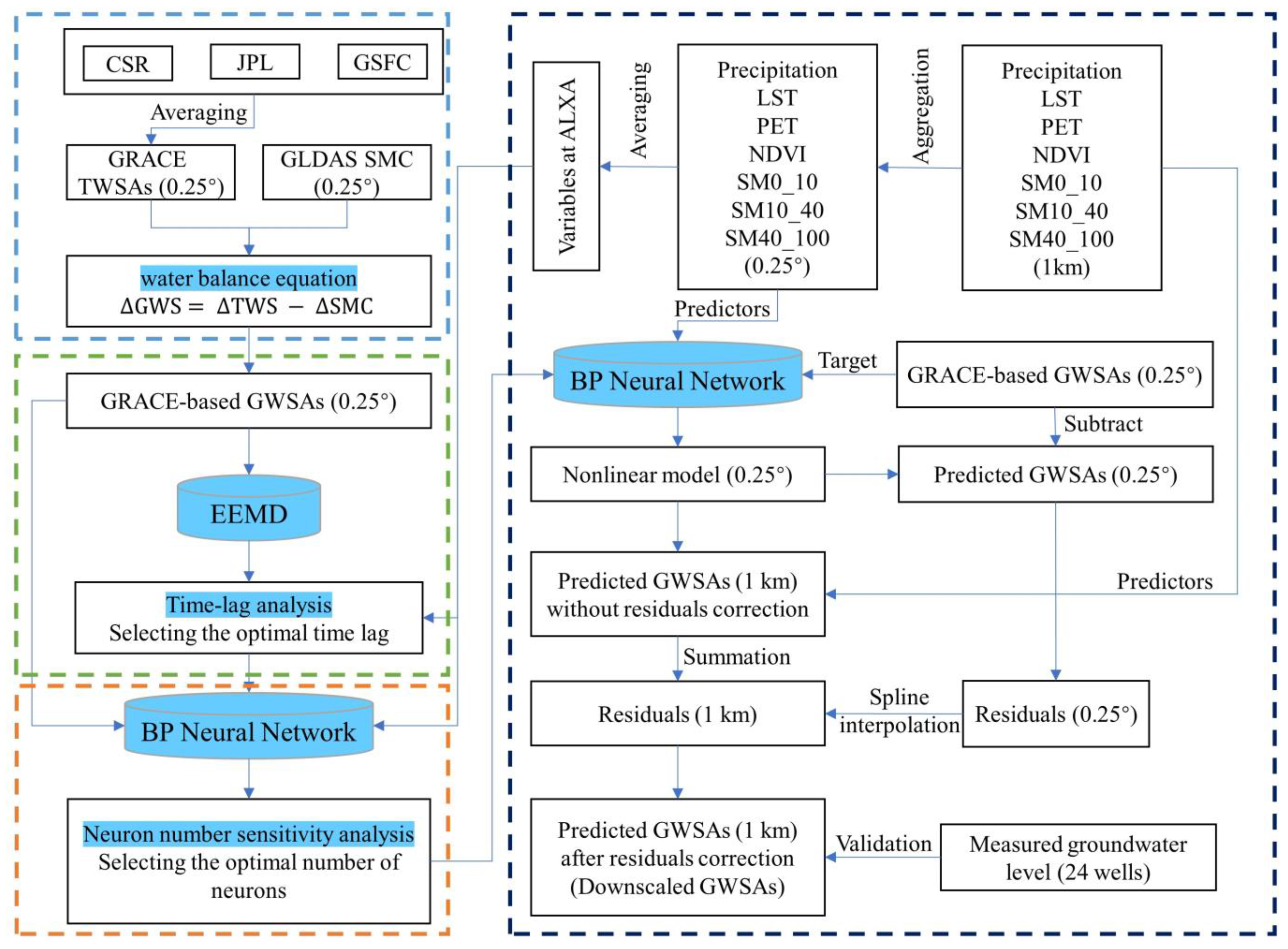
We collected data for 142 in situ groundwater monitoring wells from the local government of Alxa, but the recording periods for each well were inconsistent. The majority of in situ monitoring wells have a monitoring period of only 1 to 3 years; only 24 wells have a monitoring period of more than 10 years, so these were selected as the validation dataset. The spatial distribution of the 24 wells is shown in Figure 1b–g, and their details are shown in Table S2.

3. Methods

The overall technical route is shown in Figure 2. There are four steps for generating downscaled GWSA data: (1) isolating the GWSA component from the GRACE terrestrial water storage (TWS) anomalies (TWSAs) through WBE; (2) analyzing the time-lag effect of the input predictors on the GWSAs using the EEMD method; (3) obtaining the optimal number of hidden neurons and driving the BPNN modeling; and (4) downscaling the GRACE-based GWSAs from 0.25° to 1 km resolution based on the optimal BPNN model and validating it.

3.1. Isolating GWSAs from GRACE TWSAs

The $\mathrm{TWS} (\mathrm{cm}$) derived from the GRACE consists of the vertically integrated water storage component anomalies of the aquifer and includes surface runoff (rivers and lakes) (${\mathrm{Q}}_{\mathrm{s}}({\mathrm{kg} \mathrm{m}}^{-2})$), canopy water storage ($\mathrm{CWS} ({\mathrm{kg} \mathrm{m}}^{-2}$)), snow water equivalent ($\mathrm{SWE} ({\mathrm{kg} \mathrm{m}}^{-2})$), SMC (${\mathrm{kg} \mathrm{m}}^{-2}$), and GWS ($\mathrm{cm}$). The WBE was utilized to isolate the GWSAs from the GRACE TWSAs by subtracting other components:

$$∆\mathrm{GWS}=∆\mathrm{TWS}-∆{\mathrm{Q}}_{\mathrm{s}}-∆\mathrm{CWS}-∆\mathrm{SWE}-∆\mathrm{SMC}$$

(1)

Due to the arid climate, sparse vegetation, and shortage of land surface water resources in the study area, ${\mathrm{Q}}_{\mathrm{s}}$, CWS, and SWE are negligible in the WBE. Here, the GWS can be isolated by simply subtracting $\mathrm{SMC}$ from $\mathrm{TWS}$:

$$∆\mathrm{GWS}=∆\mathrm{TWS}-∆\mathrm{SMC}$$

(2)

The SMC estimation was provided by the GLDAS data. In addition, the GLDAS data were processed in a manner similar to that in which the GRACE anomaly data were processed, and the SMC anomaly at time t was estimated using Equation (3):

$$∆\mathrm{G}\left(\mathrm{t}\right)= \mathrm{G}\left(\mathrm{t}\right)-{ \mathrm{G}}_{\mathrm{avg} \mathrm{of} 2004-2009}$$

(3)

where $\mathrm{G}\left(\mathrm{t}\right)$ represents the SMC from the GLDAS data at time t, $∆\mathrm{G}\left(\mathrm{t}\right)$ is the SMC anomaly at time t, and ${\mathrm{G}}_{\mathrm{avg} \mathrm{of} 2004-2009}$ represents the average value of the SMC from 2004 to 2009.

3.2. Analysis of Time-Lag Effect

To investigate the time-lag effect of the GRACE-based GWSAs in response to the input predictors, we selected different lag times (no lag, 1 month, 2 months, 3 months, 4 months, and 5 months) to analyze the correlation between each input variable and the GRACE-based GWSAs [29]. The lag time with the highest correlation coefficient was used in the subsequent BPNN modeling.

There was no statistically significant correlation between the predictors and the predictand as the GRACE-based GWSAs contained obvious secular trends and had no regular annual cycle variations. However, the opposite was the case for most predictors (e.g., precipitation, LST, PET, and NDVI). Thus, EEMD, a method based on empirical mode decomposition (EMD) for time series analysis, was used to separate the secular trends in the GRACE-based GWSAs and obtain more stationary time series with annual cycles. The original time series, G(t), were decomposed into a set of amplitude-frequency-modulated oscillatory functions (intrinsic mode functions, IMFs), ${\mathrm{IMF}}_{\mathrm{i}}\left(\mathrm{t}\right)$, and a residual, R(t) (the residual represents the trend of the original time series), using EEMD:

$$\mathrm{G}\left(\mathrm{t}\right)={{\displaystyle \sum }}_{\mathrm{i}=1}^{\mathrm{n}}{\mathrm{IMF}}_{\mathrm{i}}\left(\mathrm{t}\right)+ \mathrm{R}\left(\mathrm{t}\right)$$

(4)

A fast Fourier transform (FFT) was then utilized to extract the corresponding average cycle of every IMF component. FFT spectral analysis was performed and the cycle corresponding to the maximum value of power was selected as the final average cycle of that IMF component. Next, the variance contribution rate of every IMF component was calculated to analyze the significance of the average cycle. The variance contribution rate can be calculated using Equation (6):

$${\mathrm{P}}_i=\left({\mathrm{V}}_i/{{\displaystyle \sum }}_{i=1}^n{\mathrm{V}}_i\right)\times 100\%$$

(5)

where ${\mathrm{P}}_i$ is the variance contribution rate of the $i\mathrm{th}$ IMF component, ${\mathrm{V}}_i$ is the variance of the $i\mathrm{th}$ IMF component, and $n$ is the number of IMFs. Finally, the IMF component which had an average cycle of around one year and did not have a low variance contribution rate value was selected to represent the original time series data.

However, it is not necessary to decompose GRACE-based GWSAs if the predictor also has a significant secular trend. A linear regression slope was used to determine whether there was a significant long-term trend in each predictor. As the magnitude of the predictors was different, each predictor was normalized to 0–1 to calculate the regression slope value (${\mathsf{\theta }}_{slope}$) from April 2002 to December 2020. We created a condition-based correlation analysis method to analyze the correlation between the predictors and the predictand:

$$\{\begin{array}{c}Corr\left(\mathrm{predictors},\mathrm{original} \mathrm{predictand}\right), if \left|{\mathsf{\theta }}_{slope}\right|>\omega \\ Corr\left(\mathrm{predictors},\mathrm{IMF} \mathrm{of} \mathrm{original} \mathrm{predictand}\right), if \left|{\mathsf{\theta }}_{slope}\right|\le \omega \end{array}$$

(6)

where $Corr\left(\mathrm{predictors},\mathrm{original} \mathrm{predictand}\right)$ is the CC between the predictor and the original predictand and $Corr\left(\mathrm{predictors},\mathrm{IMF} \mathrm{of} \mathrm{original} \mathrm{predictand}\right)$ is the CC between the predictor and the IMF of the original predictand. The value of ω is contingent upon the long-term trend exhibited by the predictors (for further details, please refer to Section 4.1).

3.3. BPNN Modeling and Parameter Sensitivity Analysis

A BPNN, an ANN-based machine learning model, was developed to downscale the GRACE-based GWSAs. The BPNN is one of the most widely used ANN models, capable of approximating complex nonlinear relationships between different environmental variables with limited knowledge of physical processes [48,49,50]. The structure of the neural network includes an input layer, a hidden layer, and an output layer. A neural network can have multiple hidden layers, and the hidden neurons are the neurons in the hidden layer. Neurons in the previous layer are connected to neurons in the next layer, and information from the neurons in the previous layer are collected and passed to the next layer after “activation”. The back propagation training process starts when input information reaches the output layer in sequence, and the error is passed back if the discrepancy between the output result and the expected value exceeds a given value. The neural network then gains the output value again by adjusting the weight value of the neurons and trains repeatedly until the error meets the accuracy requirements [51].

The parameter settings of the BPNN affect the accuracy of the spatial downscaling model, especially the number of hidden neurons, which is one of the most critical parameters affecting the robustness of the BPNN model [52,53]. Therefore, we mainly focused on the impact of different numbers of hidden neurons on the BPNN model’s accuracy, and a sensitivity analysis was conducted to determine the optimal number of hidden neurons. It is worth mentioning that a network with too few hidden neurons may not be powerful enough to perform a given learning task, while an excessive number of hidden neurons causes the network memorizes the training dataset and exhibit poor generalizing capabilities, resulting in unsatisfactory performance [52]. As a rule of thumb, the appropriate number of hidden neurons [54] should be calculated as follows:

$$\left(1/2\right)\times Nu{m}_{predictor}\le Nu{m}_{neuron}\le 2\times Nu{m}_{predictor}$$

(7)

where $Nu{m}_{predictor}$ is the number of input predictors and $Nu{m}_{neuron}$ is the number of hidden neurons. Therefore, the number of hidden neurons in this study was set from 3 to 14.

Additionally, the accuracy of the BPNN model is also affected by different sample ratios. Therefore, we utilized 10 different combinations of sample sizes to train the input and target variables. We found that the highest accuracy was obtained when the training–validating–testing samples were 70%–15%–15% (see Figure S2 in Supplementary Materials). In this study, we used a single hidden layer feedforward network with sigmoid hidden neurons and linear output neurons to drive our input datasets. We trained the network using the Levenberg–Marquardt backpropagation algorithm in Matlab R2018a.

3.4. Spatial Downscaling and Validation

The BPNN model was used to downscale the GRACE-based GWSA data from 0.25° to 1 km resolution, and the detailed processes are shown in Figure 2 and listed below:

(i) Seven predictors at 1 km resolution were aggregated to 0.25° resolution using pixel averaging.

(ii) Predictors at 0.25° resolution were used as independent variables, and GRACE-based GWSAs (0.25°) were utilized as the target variable. We used the BPNN algorithm to train the predictors and target variables, obtain a nonlinear regression model, and predict GWSA data at 0.25° resolution based on the optimal lag time of the GRACE-based GWSAs and the optimal number of hidden neurons.

(iii) Based on the nonlinear function obtained in Step (2), predictors at 1 km resolution were input into the nonlinear model to predict the GWSA data at 1 km resolution, leading to the preliminary downscaling result without residual correction.

(iv) The predicted GWSA data at 0.25° resolution were subtracted from the original GWSA data at 0.25° to acquire the 0.25° resolution residuals.

(v) The residuals (0.25°) were interpolated to 1 km resolution using a spline interpolation method, and the residual correction was performed at 1 km resolution by adding the residuals (1 km) to the predicted GWSAs at 1 km resolution. The predicted data after residual correction were used as the final downscaled GRACE-based GWSA data.

The downscaled GRACE-based GWSA results were then compared with the GWL data from the groundwater monitoring wells.

3.5. Evaluation Metrics

To quantify the performance of the BPNN model and downscaled GWSA data, we used the following metrics:

(i) CC, which measures the correlation between predicted variables (i.e., GWSAs predicted by the BPNN) and observed variables (i.e., GWSAs obtained from the GRACE).

$$\mathrm{CC}={{\displaystyle \sum }}_{i=1}^n\left(x_i-\overline{x}\right)\left(y_i-\overline{y}\right)/\sqrt{{{\displaystyle \sum }}_{i=1}^n{\left(x_i-\overline{x}\right)}^2{\left(y_i-\overline{y}\right)}^2}$$

(8)

(ii) The root-mean-square error (RMSE), which represents the root-mean-square error between the predicted variables and the observed variables:

$$\mathrm{RMSE}=\sqrt{\left(1/n\right){{\displaystyle \sum }}_{i=1}^n{\left(x_i-y_i\right)}^2}$$

(9)

where $\overline{x}$ and $\overline{y}$ indicate the mean values, $x_i$ is the target value, and $y_i$ is the predicted value.

4. Results

This section presents the optimal lag time results, the results of the sensitivity analysis of the parameter settings and the BPNN performance, and the results of the downscaled GRACE-based GWSAs, as well as their validation.

4.1. Optimal Lag Time Results

The original GRACE-based GWSA time series was decomposed into six IMF components (IMF1 to IMF6) and a residual function using the EEMD method, and the results are illustrated in Figure 3. The average cycle and variance contribution rate of each IMF component are listed in

Table 1. Average cycle and variance contribution rate of the six IMF components.

IMFs	Average Cycle (Month)	Variance Contribution Rate (%)
IMF1	2.9	35.3
IMF2	5.8	17.4
IMF3	11.3	11.8
IMF4	28.1	15.3
IMF5	56.3	6.1
IMF6	112.5	14.1

. We observed that IMF3, with its average cycle of 11.3 months (~a year) and its variance contribution rate of 11.8%, was the IMF component that best represented the original GRACE-based GWSA time series for correlation analysis with each input predictor. The contrastive results of IMF3 and the original GRACE-based GWSAs in terms of time variation have been plotted in Figure 4c.

Figure 4a,b illustrate the time series variation curves for each predictor. We observed strong seasonal characteristics and relatively weak secular trends in precipitation, PET, LST, NDVI, and SM0_10. We also observed weakly cyclical features and relatively weak ascending trends in SM10_40 and SM40_100. The linear regression slopes of each predictor are listed in Table S3. The regression slopes for precipitation, PET, LST, NDVI, and SM0_10 are 0.0010/year, 0.0012/year, 0.0138/year, and 0.0034/year, respectively. For SM10_40 and SM40_100, the regression slopes are 0.0245/year and 0.0305/year, respectively. The correlation coefficients between the predictors and the IMF of the original predictand are higher for precipitation, PET, LST, NDVI, and SM0_10 compared with those of the original predictand. However, this pattern is reversed for SM10_40 and SM40_100. Therefore, we established a range of $0.0138<\mathsf{\omega }<0.0245$ to differentiate whether the predictors possess a long-term trend in our study. We calculated the CC between five predictors (precipitation, etc.) and IMF3, and between two predictors (SM10_40 and SM40_100) and the original GRACE-based GWSAs, by shifting the lag time for optimal lag time analysis. Different correlations existed between the predictors and the predictand at different lag times (0 to 5 months), and the results of the lag time analysis are presented in

Table 2. CC between the input predictors and GRACE-based GWSAs or IMF3 based on different lag times.

Lag	Precipitation	LST	PET	NDVI	SM0_10	SM10_40	SM40_100
0	−0.002	0.27	0.30	−0.17	−0.23	−0.67	−0.77
1	0.27	0.56	0.58	0.14	0.10	−0.68	−0.76
2	0.47	0.70	0.70	0.41	0.41	−0.67	−0.75
3	0.54	0.66	0.64	0.58	0.61	−0.64	−0.74
4	0.47	0.44	0.41	0.60	0.64	−0.61	−0.72
5	0.28	0.10	0.07	0.47	0.51	−0.60	−0.72

. Figure S3 shows the effectiveness of using the EEMD method to perform optimal lag time analysis, and we observed that LST was almost irrelevant to the original GRACE-based GWSAs (Figure S3a). However, the CC between LST and the GRACE-based GWSAs improved from 0.02 to 0.70 when IMF3 was used in place of the original GRACE-based GWSAs. The optimal lag time of the GWSAs relative to each predictor would later be used in the BPNN model, helping to better mimic the natural environment and improve the performance of the model.

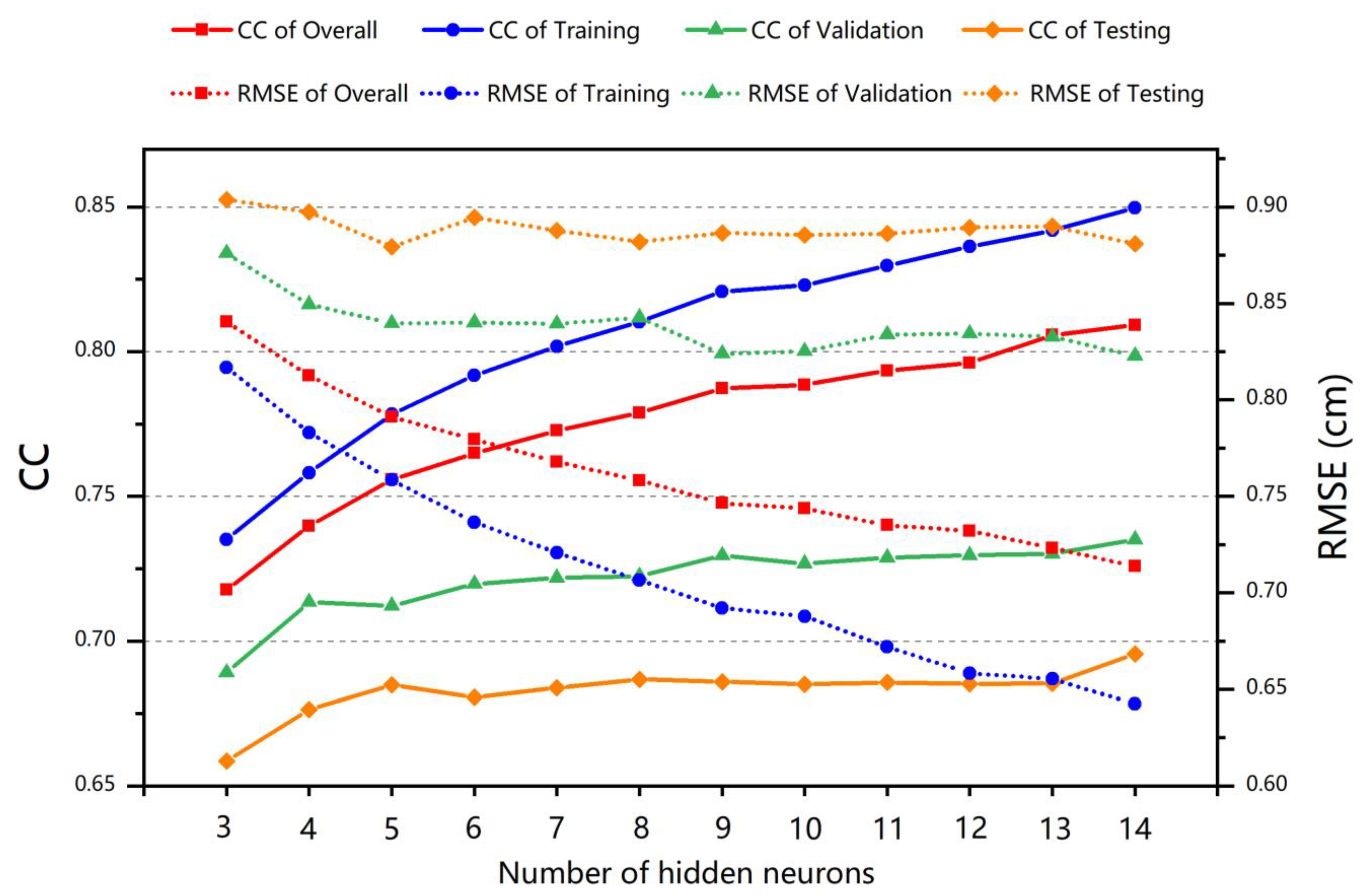
4.2. Sensitivity Analysis of the Parameter Settings and BPNN Performance

Figure 5 illustrates the results of the sensitivity analysis of the number of hidden neurons (3 to 14) in the BPNN model. The variation trend in the model accuracy for all sample types increased with the increasing number of hidden neurons. Due to this upward tendency in the BPNN’s performance with an increasing number of hidden neurons, and because 14 hidden neurons was the highest number we adopted, the best result was obtained using a network containing 14 hidden neurons. We then increased the number of hidden neurons to 20, and the results of the BPNN’s performance are shown in Figure S4. We observed that the accuracy of the validation and testing samples decreased when the number of hidden neurons was greater than 14. Although the accuracy of the overall samples and the training samples increased continuously, the decreasing accuracy of the validation samples and testing samples had a negative impact on the accuracy of the BPNN. Therefore, we adopted 14 hidden neurons for all networks.

The BPNN model accuracy results for each month are shown in Figure 6. We trained the same BPNN model 100 times to obtain the result with the highest precision. The mean CC for all months was 0.81 for the overall samples, 0.85 for the training samples, 0.74 for the validation samples, and 0.70 for the testing samples, while the mean RMSE for all months was 0.70 cm for the overall samples, 0.63 cm for the training samples, 0.81 cm for the validation samples, and 0.87 cm for the testing samples. The model performance of the BPNN was mainly reflected in the accuracy of the overall samples. The simulation of the GWSAs using the BPNN model generally achieved good results for all months (with a mean CC of 0.81 and mean RMSE of 0.70 cm).

4.3. Downscaling of GRACE-Based GWSAs

This section contains the results of the downscaled GRACE-based GWSAs and a comparison of the spatial and temporal variations of the GWSAs before and after downscaling.

4.3.1. Comparison of Temporal Variation

The downscaled GWSAs provided a sufficiently fine resolution to understand the temporal variation in the GWS of Alxa League. Figure 7 shows the spatial distribution of the downscaled GWSAs from 2002 to 2020. The GWS of Alxa generally dropped from 2002 to 2020, and the hotspots of GWS decline were more visible in Left Banner, followed by Right Banner and Ejina Banner. GWS decline was higher in the southeast areas compared with the northwest parts of Alxa, and this can mainly be attributed to the higher population (about 78% of the population of Alxa) and higher amount of irrigation land (about 68% of the farmland in Alxa) in Left Banner, where the consumptive fraction of irrigation withdrawal was larger and mainly supplied by groundwater. We observed that the GWS decreased more rapidly after 2006. We already know that there were no secular trends in climate drivers, including precipitation, evapotranspiration, and temperature (Figure 4); therefore, the persistent long-term decline (generally more than 10 years) of GWS was mostly attributed to anthropogenic activities, such as excess groundwater abstraction for irrigation and industrial production.

The downscaled GWSAs retained their original spatial distribution characteristics and simultaneously showed more spatially detailed information at a smaller scale. To further validate the effectiveness of the downscaled GWSAs, we compared the long-term variation trends of the original GWSAs and the downscaled GWSAs from April 2002 to December 2020. The results are shown in Figure 8. We observed that the variation trends were very similar between the two datasets; the GWS decline rate in Alxa was about −0.40 cm/year for both the original GWSAs and the downscaled GWSAs. The GWS decline rate was higher in Left Banner (with an average trend of −0.45 cm/year), followed by Right Banner (with a mean trend of −0.40 cm/year) and Ejina Banner (with an average trend of −0.35 cm/year).

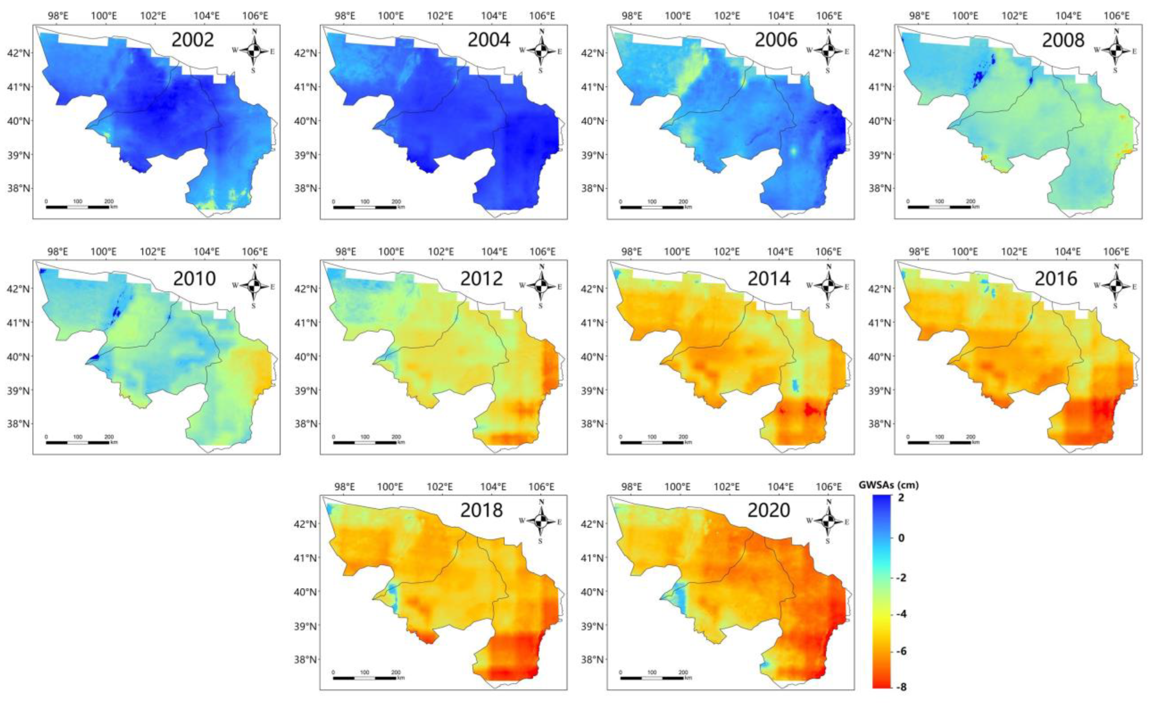
4.3.2. Comparison of Spatial Distribution

To examine the spatially detailed features and spatial distribution differences of the downscaled GWSAs, we chose two points, P1 and P2, with a distance of about 130 km (covering 5 pixels of the original GWSA data and 130 pixels of the downscaled GWSA data) and utilized the P1–P2 transect to demonstrate how the spatial downscaling method improves the estimation of GWSAs at small scales within the three banners. Figure 9 contrasts the spatial distributions of the original GWSAs with those of the downscaled GWSAs in Left Banner (January 2004), Right Banner (July 2016), and Ejina Banner (April 2009). The variations in the spatial distributions of the downscaled GWSAs appeared to be consistent with those of the original GWSAs. For example, the GWSAs of Ejina Banner in January 2004 exhibited a lower increase in the upstream of the Heihe river basin which was presented as uniform in both the original GWSAs and the downscaled GWSAs. The spatial variation of the original GWSAs along the P1–P2 transect closely matched that of the downscaled GWSAs; however, the downscaled GWSA data could reflect strong spatial heterogeneity and convey more detailed features.

4.4. Validation of Downscaled GWSAs

The downscaled GWSAs were validated using measured GWL data from 24 in situ groundwater monitoring wells. Figure 10 shows the correlation between the downscaled GWSAs and the observational GWL of the 24 groundwater wells. There were 12 wells whose CCs were greater than 0.6, and the average CC of the 24 wells was 0.53. In general, downscaled GWSAs were highly consistent with the observational GWL, indicating that our downscaling method can be used to construct GWSAs at the kilometer scale. A temporal variation comparison of the downscaled GWSAs against the observational GWL at a monthly scale is illustrated in Figure S5. The downscaled GWSAs and the observational GWL presented a decreasing temporal trend in most of the groundwater wells. Only certain groundwater wells (well IDs: 3, 10, 11, 12, and 13) exhibited inconsistencies in temporal trend between the downscaled GWSAs and the observational GWL.

5. Discussion

In this section, we first outline a comparative experiment that was conducted to verify the effect of lag time on the accuracy of the BPNN model. We then discuss the influence of the number of hidden neurons on the accuracy of the BPNN model. Finally, we discuss the limitations of the method proposed in our article and possible directions for future research.

5.1. Influence of Time-Lag Effect

In general, ours is an effective way to downscale GRACE data and construct GWSAs with a higher resolution using data-driven methods. Many scholars have successfully downscaled GRACE-based GWSAs to the kilometer scale in different areas around the world. However, most such studies that have been conducted in arid regions have neglected to consider the time-lag effect of the groundwater caused by the large vadose zone, and this has resulted in relatively poor modeling accuracy [23,28,55,56]. Groundwater recharge is affected by surface environmental variables only after a delay as deep drainage traverses the vadose zone before reaching the underground aquifer [57]. Because of this, our study took the time-lag effect of GWSAs into consideration to improve the accuracy of downscaling models. The optimal GWSA lag time relative to the input predictors was found by changing the lag time from 0 months to 5 months to obtain the maximum correlation between the GWSAs and the input variables. Precipitation, one of the main sources of groundwater recharge in arid regions [58], was found to be the most relevant to GWSAs with a lag time of 3 months (see Table 2) [57,59,60]. SMC (soil moisture in soil depths $\ge$ 40 cm) was strongly correlated with GWSAs, exhibiting the smallest lag time (0 to 1 month), indicating that GWS responds more immediately to deep SMC than to other input predictors. One reason for this might be that deep SMC has a shorter infiltration path, and groundwater can be directly recharged by deep SMC [61,62].

To further verify the effect of lag time on the accuracy of the model, a comparative analysis experiment was performed by both applying and not applying the optimal lag time in the model. Generally, the simulation results obtained using the optimal lag time were better. The most significant improvement in model accuracy was obtained for autumn (the results are presented in Figure 11), e.g., November, with exhibited the most obvious improvement in simulation performance of all months (overall CC: 0.82 vs. 0.78; overall RMSE: 0.70 cm vs. 0.76 cm). The next most significant improvement was obtained for summer, while the accuracy improvement was insignificant for winter and spring. Changes in GWS are more closely correlated with the climate, vegetation, and soil conditions that existed several months earlier, so the large discrepancy (most of the precipitation in Alxa occurs from June to September) in groundwater recharge rates between two seasons (e.g., summer and autumn) makes it more important to consider the time-lag effect for BPNN modeling. Therefore, it is crucial to consider the time-lag effect when conducting GRACE spatial downscaling studies using data-driven methods, especially in arid regions with distinct rainy and dry seasons.

5.2. Influence of Number of Hidden Neurons

The number of neurons in the hidden layer is one of the most critical parameters affecting the performance and reliability of the BPNN model. Our study mainly considered the effect of varying the number of hidden neurons to further improve the accuracy of the model. Various neural networks with different numbers of hidden neurons were used, and the best neural network among them was selected based on minimized RMSE. Nevertheless, there is no commonly accepted method to determine the optimal number of hidden neurons. For example, the number of hidden neurons can be set to two-thirds of the number of input predictors [63], the square root of the sum of the number of input predictors and output variables, adding a varying constant [64], or an amount lower than twice the number of input predictors [54]. In our study, we followed a rule of thumb by setting the number of hidden neurons within a range from half to twice the number of input predictors (3–14 nodes). We found that the BPNN modeling accuracy improved as the number of hidden neurons increased, a trend that has also been found in other research [54,65]. A neural network with a higher number of hidden neurons yields more accurate results and can model more complicated nonlinear relationships; however, the risk of overfitting is also increased [66]. Thus, we adopted 14 hidden neurons for all neural networks to obtain higher accuracy.

5.3. Limitations of the Method and Perspectives

Although the BPNN is a feasible and effective method for downscaling GRACE-based GWSAs to 1 km resolution while taking into consideration the time-lag effect of the GWSAs and the optimal number of hidden neurons, our proposed spatial downscaling method could be further modified by addressing the following limitations in future research.

Firstly, our study area was confined to Alxa, a relatively small, arid region, so we did not analyze the local spatial differences in the time-lag effect resulting from the spatial heterogeneity of meteorological, hydrological, or topographical variables. However, the lag time of GWSAs should be analyzed in depth in GRACE downscaling studies using data-driven methods in which the spatial scope is extended to larger national or continental scales. For instance, GWS may be replenished more rapidly owing to extreme precipitation events in local areas.

Secondly, a scarcity of observational materials and validated datasets is a common problem for arid regions. Therefore, the downscaled GWSAs in our study were validated using only 24 in situ monitoring groundwater wells due to the limited GWL data in Alxa. Moreover, the spatial distribution of groundwater wells was very uneven in this study area. This being the case, it was difficult to validate our constructed 1 km resolution GWSA product comprehensively. Therefore, to improve the generalizability of downscaling models, a zonal modeling approach could be adopted to simulate GWSAs in local areas with relatively adequate groundwater wells, and then the study could be extended to the whole study area.

Finally, in terms of the selection of input predictors, only precipitation, PET, LST, NDVI, and SMC were used in our study. These predictors were considered adequate to represent the important physical processes in the terrestrial water cycle, and they strongly correlated with the GRACE-based GWSA data [25]. However, groundwater recharge rates in Alxa are also affected by anthropogenic activities, as was discussed in Section 4.3.1. We therefore added gridded gross domestic product (GDP) distribution and population density (PD), two predictors reflecting human intervention, to the BPNN model to compare its performance with that of the model when trained using only natural predictors. The results showed that the accuracy of the downscaling model that considered GDP and PD was lower, with CC values of 0.80 vs. 0.81 (overall), 0.84 vs. 0.85 (training), 0.72 vs. 0.74 (validation), and 0.67 vs. 0.70 (testing). This proves that gridded GDP and PD datasets are not suitable as input predictors in Alxa, where human intervention is concentrated in localized areas. In addition, further variables, including topographical, geological, and positional factors, could be integrated if the study area were expanded to larger national and continental scales. Multi-variable inputs may further improve the simulated accuracy of GRACE downscaling research by adopting data-driven methods.

6. Conclusions

Our study proposed a novel spatial downscaling method for constructing GRACE-based 1 km resolution GWSAs by adopting a BPNN model that considered the time-lag effect and the optimal number of hidden neurons, and which was validated in Alxa League, an arid region of northwestern China. The downscaling model achieved good simulation performance with a mean CC of 0.81 and a mean RMSE of 0.70 cm for all months from April 2002 to December 2020. We found that the time-lag effect and the optimal number of hidden neurons greatly impact the performance of the model. Specifically, the simulation performance of the model considering the optimal lag time was generally better, especially for autumn due to the large discrepancy in groundwater recharge rates between summer and autumn. For instance, the most significant improvement in model accuracy occurred in November, with a contrastive overall CC of 0.82 vs. 0.78 and an overall RMSE of 0.70 cm vs. 0.76 cm. In addition, a neural network considering the optimal number of hidden neurons (14 neurons) yielded more accurate modeling results. Furthermore, our downscaled GWSA results were highly consistent with the original data in terms of long-term temporal variations and spatial distribution. The GWS decline rate in Alxa was about −0.40 ± 0.01 cm/year for both the original and downscaled GWSA data, and the downscaled data reflected strong spatial heterogeneity and conveyed more spatially detailed features. In general, we have provided a feasible and effective approach for downscaling GRACE data to smaller scales, though there is still room for improvement in future studies. For instance, local spatial differences in the time-lag effect need to be analyzed in depth due to spatial heterogeneity, the zonal modeling approach can be adopted to simulate GWSAs, and additional environmental variables (e.g., topographical, geological, and positional factors) can be involved if the study area is expanded to larger national and continental scales in future research.

References

1. Esterhuyse, S.; Vermeulen, D.; Glazewski, J. Regulations to protect groundwater resources during unconventional oil and gas extraction using fracking. Wiley Interdiscip. Rev. Water 2019, 6, e1382. [Google Scholar] [CrossRef]
2. Famiglietti, J. The global groundwater crisis. Nat. Clim. Chang. 2014, 4, 945–948. [Google Scholar] [CrossRef] [Green Version]
3. Wang, S.; Liu, H.; Yu, Y.; Zhao, W.; Yang, Q.; Liu, J. Evaluation of groundwater sustainability in the arid Hexi Corridor of Northwestern China, using GRACE, GLDAS and measured groundwater data products. Sci. Total Environ. 2020, 705, 135829. [Google Scholar] [CrossRef]
4. Wang, W.; Chen, Y.; Wang, W.; Jiang, J.; Cai, M.; Xu, Y. Evolution characteristics of groundwater and its response to climate and land-cover changes in the oasis of dried-up river in Tarim Basin. J. Hydrol. 2021, 594, 125644. [Google Scholar] [CrossRef]
5. Long, D.; Yang, W.; Scanlon, B.; Zhao, J.; Liu, D.; Burek, P.; Pan, Y.; You, L.; Wada, Y. South-to-North Water Diversion stabilizing Beijing’s groundwater levels. Nat. Commun. 2021, 13, 5. [Google Scholar] [CrossRef]
6. Massoud, E.; Liu, Z.; Shaban, A.; El Hage, M. Groundwater Depletion Signals in the Beqaa Plain, Lebanon: Evidence from GRACE and Sentinel-1 Data. Remote Sens. 2018, 10, 143. [Google Scholar] [CrossRef]
7. Bhering, A.; Antunes, I.; Marques, E.; de Paula, R. Geological and hydrogeological review of a semi-arid region with conflicts to water availability (southeastern Brazil). Environ. Res. 2021, 202, 111756. [Google Scholar] [CrossRef] [PubMed]
8. Narvaez-Montoya, C.; Torres-Martinez, J.; Pino-Vargas, E.; Cabrera-Olivera, F.; Loge, F.; Mahlknecht, J. Predicting adverse scenarios for a transboundary coastal aquifer system in the Atacama Desert (Peru/Chile). Sci. Total Environ. 2022, 806, 150386. [Google Scholar] [CrossRef] [PubMed]
9. Neves, M.; Nunes, L.; Monteiro, J. Evaluation of GRACE data for water resource management in Iberia: A case study of groundwater storage monitoring in the Algarve region. J. Hydrol. Reg. Stud. 2020, 32, 100734. [Google Scholar] [CrossRef]
10. Wang, F.; Wang, Z.; Yang, H.; Di, D.; Zhao, Y.; Liang, Q. Utilizing GRACE-based groundwater drought index for drought characterization and teleconnection factors analysis in the North China Plain. J. Hydrol. 2020, 585, 124849. [Google Scholar] [CrossRef]
11. Massoud, E.; Purdy, A.; Miro, M.; Famiglietti, J. Projecting groundwater storage changes in California’s Central Valley. Sci. Rep. 2018, 8, 12917. [Google Scholar] [CrossRef]
12. Massoud, E.; Turmon, M.; Reager, J.; Hobbs, J.; Liu, Z.; David, C.H. Cascading Dynamics of the Hydrologic Cycle in California Explored through Observations and Model Simulations. Geosciences 2020, 10, 71. [Google Scholar] [CrossRef] [Green Version]
13. Ali, S.; Liu, D.; Fu, Q.; Cheema, M.; Pal, S.; Arshad, A.; Pham, Q.; Zhang, L. Constructing high-resolution groundwater drought at spatio-temporal scale using GRACE satellite data based on machine learning in the Indus Basin. J. Hydrol. 2022, 612, 128295. [Google Scholar] [CrossRef]
14. Pascal, C.; Ferrant, S.; Selles, A.; Marechal, J.; Paswan, A.; Merlin, O. Evaluating downscaling methods of GRACE (Gravity Recovery and Climate Experiment) data: A case study over a fractured crystalline aquifer in southern India. Hydrol. Earth Syst. Sci. 2022, 26, 4169–4186. [Google Scholar] [CrossRef]
15. Fatolazadeh, F.; Eshagh, M.; Goita, K. New spectro-spatial downscaling approach for terrestrial and groundwater storage variations estimated by GRACE models. J. Hydrol. 2022, 615, 128635. [Google Scholar] [CrossRef]
16. Fatolazadeh, F.; Eshagh, M.; Goïta, K.; Wang, S. A New Spatiotemporal Estimator to Downscale GRACE Gravity Models for Terrestrial and Groundwater Storage Variations Estimation. Remote Sens. 2022, 14, 5991. [Google Scholar] [CrossRef]
17. Schumacher, M.; Forootan, E.; van Dijk, A.; Mueller Schmied, H.; Crosbie, R.; Kusche, J.; Doll, P. Improving drought simulations within the Murray-Darling Basin by combined calibration/assimilation of GRACE data into the WaterGAP Global Hydrology Model. Remote Sens. Environ. 2018, 204, 212–228. [Google Scholar] [CrossRef] [Green Version]
18. Shokri, A.; Walker, J.; van Dijk, A.; Pauwels, V. On the Use of Adaptive Ensemble Kalman Filtering to Mitigate Error Misspecifications in GRACE Data Assimilation. Water Resour. Res. 2019, 55, 7622–7637. [Google Scholar] [CrossRef] [Green Version]
19. Tangdamrongsub, N.; Steele-Dunne, S.; Gunter, B.; Ditmar, P.; Sutanudjaja, E.; Sun, Y.; Xia, T.; Wang, Z. Improving estimates of water resources in a semi-arid region by assimilating GRACE data into the PCR-GLOBWB hydrological model. Hydrol. Earth Syst. Sci. 2017, 21, 2053–2074. [Google Scholar] [CrossRef] [Green Version]
20. Nie, W.; Zaitchik, B.; Rodell, M.; Kumar, S.; Arsenault, K.; Li, B.; Getirana, A. Assimilating GRACE Into a Land Surface Model in the Presence of an Irrigation-Induced Groundwater Trend. Water Resour. Res. 2019, 55, 11274–11294. [Google Scholar] [CrossRef]
21. Arshad, A.; Mirchi, A.; Samimi, M.; Ahmad, B. Combining downscaled-GRACE data with SWAT to improve the estimation of groundwater storage and depletion variations in the Irrigated Indus Basin (IIB). Sci. Total Environ. 2022, 838, 156044. [Google Scholar] [CrossRef]
22. Yin, W.; Zhang, G.; Liu, F.; Zhang, D.; Zhang, X.; Chen, S. Improving the spatial resolution of GRACE-based groundwater storage estimates using a machine learning algorithm and hydrological model. Hydrogeol. J. 2022, 30, 947–963. [Google Scholar] [CrossRef]
23. Zuo, J.; Xu, J.; Chen, Y.; Li, W. Downscaling simulation of groundwater storage in the Tarim River basin in northwest China based on GRACE data. Phys. Chem. Earth 2021, 123, 103042. [Google Scholar] [CrossRef]
24. Yin, W.; Fan, Z.; Tangdamrongsub, N.; Hu, L.; Zhang, M. Comparison of physical and data-driven models to forecast groundwater level changes with the inclusion of GRACE—A case study over the state of Victoria, Australia. J. Hydrol. 2021, 602, 126735. [Google Scholar] [CrossRef]
25. Mas, J.; Flores, J. The application of artificial neural networks to the analysis of remotely sensed data. Int. J. Remote Sens. 2008, 29, 617–663. [Google Scholar] [CrossRef]
26. Odebiri, O.; Odindi, J.; Mutanga, O. Basic and deep learning models in remote sensing of soil organic carbon estimation: A brief review. Int. J. Appl. Earth Obs. Geoinf. 2021, 102, 102389. [Google Scholar] [CrossRef]
27. Ali, S.; Liu, D.; Fu, Q.; Cheema, M.; Pham, Q.; Rahaman, M.; Dang, T.; Anh, D. Improving the Resolution of GRACE Data for Spatio-Temporal Groundwater Storage Assessment. Remote Sens. 2021, 13, 3513. [Google Scholar] [CrossRef]
28. Miro, M.; Famiglietti, J. Downscaling GRACE Remote Sensing Datasets to High-Resolution Groundwater Storage Change Maps of California’s Central Valley. Remote Sens. 2018, 10, 143. [Google Scholar] [CrossRef] [Green Version]
29. Seyoum, W.; Milewski, A. Improved methods for estimating local terrestrial water dynamics from GRACE in the Northern High Plains. Adv. Water Resour. 2017, 110, 279–290. [Google Scholar] [CrossRef]
30. Jie, F.; Fei, L.; Li, S.; Hao, K.; Liu, L.; Zhu, H. Prediction model for irrigation return flow considering lag effect for arid areas. Agric. Water Manag. 2021, 256, 112559. [Google Scholar] [CrossRef]
31. de Vries, J.; Simmers, I. Groundwater recharge: An overview of processes and challenges. Hydrogeol. J. 2002, 10, 5–17. [Google Scholar] [CrossRef]
32. Zhe, M.; Zhang, X. Time-lag effects of NDVI responses to climate change in the Yamzhog Yumco Basin, South Tibet. Ecol. Indic. 2021, 124, 107431. [Google Scholar] [CrossRef]
33. Liu, B.; Zou, X.; Yi, S.; Sneeuw, N.; Cai, J.; Li, J. Identifying and separating climate- and human-driven water storage anomalies using GRACE satellite data. Remote Sens. Environ. 2021, 263, 112559. [Google Scholar] [CrossRef]
34. Wang, J.; Xu, D. Artificial Neural Network-Based Microwave Satellite Soil Moisture Reconstruction over the Qinghai-Tibet Plateau, China. Remote Sens. 2021, 13, 5156. [Google Scholar] [CrossRef]
35. Zhou, L.; Luo, T.; Du, M.; Chen, Q.; Liu, Y.; Zhu, Y.; He, C.; Wang, S.; Yang, K. Machine Learning Comparison and Parameter Setting Methods for the Detection of Dump Sites for Construction and Demolition Waste Using the Google Earth Engine. Remote Sens. 2021, 13, 787. [Google Scholar] [CrossRef]
36. Feng, Q.; Tian, Y.; Yu, T.; Yin, Z.; Cao, S. Combating desertification through economic development in northwestern China. Land Degrad. Dev. 2019, 30, 910–917. [Google Scholar] [CrossRef]
37. Wei, Y.; Chen, D.; White, R.; Willett, I.; Edis, R.; Langford, J. Farmers’ perception of environmental degradation and their adoption of improved management practices in alxa, China. Land Degrad. Dev. 2009, 20, 336–346. [Google Scholar] [CrossRef]
38. Vasco, D.; Kim, K.; Farr, T.; Reager, J.; Bekaert, D.; Sangha, S.; Rutqvist, J.; Beaudoing, H. Using Sentinel-1 and GRACE satellite data to monitor the hydrological variations within the Tulare Basin, California. Sci. Rep. 2022, 12, 3867. [Google Scholar] [CrossRef]
39. Save, H.; Bettadpur, S.; Tapley, B. High-resolution CSR GRACE RL05 mascons. J. Geophys. Res. Solid Earth 2016, 121, 7547–7569. [Google Scholar] [CrossRef]
40. Save, H. CSR GRACE and GRACE-FO RL06 Mascon Solutions v02; University of Texas: Austin, TX, USA, 2020. [Google Scholar]
41. Watkins, M.; Wiese, D.; Yuan, D.; Boening, C.; Landerer, F. Improved methods for observing Earth’s time variable mass distribution with GRACE using spherical cap mascons. J. Geophys. Res. Solid Earth 2015, 120, 2648–2671. [Google Scholar] [CrossRef]
42. Wiese, D.; Landerer, F.; Watkins, M. Quantifying and reducing leakage errors in the JPL RL05M GRACE mascon solution. Water Resour. Res. 2016, 52, 7490–7502. [Google Scholar] [CrossRef]
43. Loomis, B.; Luthcke, S.; Sabaka, T. Regularization and error characterization of GRACE mascons. J. Geod. 2019, 93, 1381–1398. [Google Scholar] [CrossRef]
44. Shouzhang, P. 1-km Monthly Precipitation Dataset for China (1901–2021); National Tibetan Plateau Data Center: Beijing, China, 2020. [Google Scholar]
45. Shouzhang, P. 1 km Monthly Potential Evapotranspiration Dataset in China (1990–2021); National Tibetan Plateau Data Center: Beijing, China, 2022. [Google Scholar]
46. Wan, Z.; Hook, S.; Hulley, G. MODIS/Terra Land Surface Temperature/Emissivity 8-Day L3 Global 1km SIN Grid V061; NASA EOSDIS Land Processes DAAC: Greenbelt, MD, USA, 2021.
47. Didan, K. MOD13A3 MODIS/Terra Vegetation Indices Monthly L3 Global 1km SIN Grid V006; NASA EOSDIS Land Processes DAAC: Greenbelt, MD, USA, 2015.
48. Han, X.; Xiong, X.; Duan, F. A new method for image segmentation based on BP neural network and gravitational search algorithm enhanced by cat chaotic mapping. Appl. Intell. 2015, 43, 855–873. [Google Scholar] [CrossRef]
49. Rumelhart, D.; Hinton, G.; Williams, R. Learning Representations by Back-Propagating Errors. Nature 1986, 323, 533–536. [Google Scholar] [CrossRef]
50. Sun, W.; Huang, C. A carbon price prediction model based on secondary decomposition algorithm and optimized back propagation neural network. J. Clean. Prod. 2019, 243, 118671. [Google Scholar] [CrossRef]
51. Zhang, L.; Wu, K.; Zhong, Y.; Li, P. A new sub-pixel mapping algorithm based on a BP neural network with an observation model. Neurocomputing 2008, 71, 2046–2054. [Google Scholar] [CrossRef]
52. Cicek, Z.; Ozturk, Z. Optimizing the artificial neural network parameters using a biased random key genetic algorithm for time series forecasting. Appl. Soft Comput. 2021, 102, 107091. [Google Scholar] [CrossRef]
53. Gocken, M.; Ozcalici, M.; Boru, A.; Dosdogru, A. Integrating metaheuristics and Artificial Neural Networks for improved stock price prediction. Expert Syst. Appl. 2016, 44, 320–331. [Google Scholar] [CrossRef]
54. Aladag, C.; Kayabasi, A.; Gokceoglu, C. Estimation of pressuremeter modulus and limit pressure of clayey soils by various artificial neural network models. Neural Comput. Appl. 2012, 23, 333–339. [Google Scholar] [CrossRef]
55. Sun, J.; Hu, L.; Liu, X.; Sun, K. Enhanced Understanding of Groundwater Storage Changes under the Influence of River Basin Governance Using GRACE Data and Downscaling Model. Remote Sens. 2022, 14, 4719. [Google Scholar] [CrossRef]
56. Zhang, J.; Liu, K.; Wang, M. Downscaling Groundwater Storage Data in China to a 1-km Resolution Using Machine Learning Methods. Remote Sens. 2021, 13, 523. [Google Scholar] [CrossRef]
57. Luo, Z.; Yong, C.; Fan, J.; Shao, M.; Wang, S.; Jin, M. Precipitation recharges the shallow groundwater of check dams in the loessial hilly and gully region of China. Sci. Total Environ. 2020, 742, 140625. [Google Scholar] [CrossRef]
58. McKenna, O.; Sala, O. Groundwater recharge in desert playas: Current rates and future effects of climate change. Environ. Res. Lett. 2018, 13, 014025. [Google Scholar] [CrossRef]
59. Qi, X.; Wang, Y.; Yang, L.; Liu, Z.; Wang, W.; Li, W. Time lags variance of groundwater level response to precipitation of Jinan karst spring watershed in recent 50 years. Carsol. Sin. 2016, 35, 384–393. [Google Scholar]
60. Yang, T.; Wang, G. Periodic variations of rainfall, groundwater level and dissolved radon from the perspective of wavelet analysis: A case study in Tengchong, southwest China. Environ. Earth Sci. 2021, 80, 492. [Google Scholar] [CrossRef]
61. Cao, G.; Scanlon, B.; Han, D.; Zheng, C. Impacts of thickening unsaturated zone on groundwater recharge in the North China Plain. J. Hydrol. 2016, 537, 260–270. [Google Scholar] [CrossRef]
62. Lu, X.; Jin, M.; van Genuchten, M.; Wang, B. Groundwater Recharge at Five Representative Sites in the Hebei Plain, China. Groundwater 2011, 49, 286–294. [Google Scholar] [CrossRef]
63. Boger, Z.; Guterman, H. Knowledge extraction from artificial neural networks models. In Proceedings of the 1997 IEEE International Conference on Systems, Man, and Cybernetics, Computational Cybernetics and Simulation, Orlando, FL, USA, 12–15 October 1997; Volume 4, pp. 3030–3035. [Google Scholar]
64. Yang, N.; Liu, L.; Xiang, D.; Fan, Q. Applying BP Neural Network to Estimate Soil Moisture with Meteorologic Parameters. Chin. J. Soil Sci. 2011, 42, 1324–1329. [Google Scholar]
65. Collins, W.; Tissot, P. An artificial neural network model to predict thunderstorms within 400 km (2) South Texas domains. Meteorol. Appl. 2015, 22, 650–665. [Google Scholar] [CrossRef]
66. Alibakshi, A. Strategies to develop robust neural network models: Prediction of flash point as a case study. Anal. Chim. Acta 2018, 1026, 69–76. [Google Scholar] [CrossRef]
Figure 1. Overview of the study area—Alxa League, China. (a) Geographical view of Alxa via a DEM map. (bg) Distribution of 24 in situ groundwater wells and GRACE pixels with 0.25° resolution.
Remotesensing 15 02913 g001
Figure 2. Flowchart of the downscaling process for GRACE-based GWSAs.
Remotesensing 15 02913 g002
Figure 3. EEMD results for GRACE-based GWSA time series.
Remotesensing 15 02913 g003
Figure 4. Time series of variables from 2002 to 2020. (a) Precipitation, LST, PET, and NDVI. (b) SM0_10, SM10_40, and SM40_100. (c) IMF3 and the original GRACE-based GWSAs.
Remotesensing 15 02913 g004
Figure 5. Results of the sensitivity analysis of different numbers of hidden neurons (3 to 14).
Remotesensing 15 02913 g005
Figure 6. BPNN simulation accuracy for all months from April 2002 to December 2020. (a) CC. (b) RMSE.
Remotesensing 15 02913 g006
Figure 7. Spatial distribution of downscaled GWSAs from 2002 to 2020.
Remotesensing 15 02913 g007
Figure 8. GWS temporal variation trends in Alxa. (a) Variation trends of the original GRACE-based GWSAs (b) Variation trends of the downscaled GWSAs.
Remotesensing 15 02913 g008
Figure 9. Spatial distribution of GWSAs before and after downscaling in the three banners of Alxa. (a) Original GWSAs in Ejina Banner. (b) Downscaled GWSAs in Ejina Banner. (c) Original GWSAs in Right Banner. (d) Downscaled GWSAs in Right Banner. (e) Original GWSAs in Left Banner. (f) Downscaled GWSAs in Left Banner.
Remotesensing 15 02913 g009
Figure 10. CCs between downscaled GWSAs and observational GWL for the 24 wells.
Remotesensing 15 02913 g010
Figure 11. Results of the contrastive analysis experiment for autumn (average of September, October, and November) in which the optimal lag time was both applied and not applied in the BPNN modeling process. (a) CC. (b) RMSE.
Remotesensing 15 02913 g011