GNSS-Based Driver Assistance for Charging Electric City Buses: Implementation and Lessons Learned from Field Testing

Abstract

Modern public transportation in urban areas increasingly relies on high-capacity buses. At the same time, the share of electric vehicles is increasing to meet environmental standards. This introduces problems when charging these vehicles from chargers at bus stops, as untrained drivers often find it difficult to execute docking manoeuvres on the charger. A practical solution to this problem requires a suitable advanced driver-assistance system (ADAS), which is a system used to automatise and make safer some of the tasks involved in driving a vehicle. In the considered case, ADAS supports docking to the electric charging station, and thus, it must solve two issues: precise positioning of the bus relative to the charger and motion planning in a constrained space. This paper addresses these issues by employing GNSS-based positioning and optimisation-based planning, resulting in an affordable solution to the ADAS for the docking of electric buses while recharging. We focus on the practical side of the system, showing how the necessary features were attained at a limited hardware and installation cost, also demonstrating an extensive evaluation of the fielded ADAS for an operator of public transportation in the city of Poznań in Poland.

1. Introduction

Efficient transportation is a growing problem in modern cities. This concerns the insufficient capacity of urban roads and the pollution generated by internal combustion vehicles. The solution to both problems at an acceptable cost can be the use of electric city buses with large capacity, which are an efficient and environmentally friendly means of transportation in large cities [1]. According to the comparative analysis of four types of urban bus powertrains: internal combustion engine, fuel cell hybrid electric vehicle, hybrid electric vehicle, and battery electric vehicle [2], the electric vehicles are markedly superior in terms of energy and environmental performance. However, a significant problem associated with the operation of such buses is the need to frequently recharge the batteries en route. This is most often accomplished by docking the bus with a pantograph to chargers set up at bus stops or in bus depot areas. The docking operation is not easy for less experienced drivers, especially when the pantograph is located in the rear of a long vehicle. Lack of experience in manoeuvring a long bus means that the docking manoeuvre is often unsuccessful the first time, and successful docking might require several attempts. Moreover, in many real-world scenarios, reversing under the charger is not allowed due to safety concerns with a long vehicle. In such cases, the driver has to omit the charging possibility, continuing driving until the next charging opportunity (i.e., the next charging station along the route), or they have to repeat the entire manoeuvre [3]. Obviously, repeating the manoeuvre takes time and may cause the bus on the route to be delayed in relation to the timetable. Although both the charger’s head and the pantograph allow for some mechanical adaptation to ensure proper connection, repeated inaccurate docking manoeuvres impose additional strain on the connecting components and can contribute to the faster wear of the collector strips and other components.

An advanced driver-assistance system (ADAS) can solve the problem by providing visual cues to the driver. Following these cues, the driver can steer the vehicle along a proper trajectory ending in a position convenient for docking. The ADAS adheres to the Society of Automotive Engineers (SAE) automation level 1 [4]. Although a bus with ADAS is not autonomous, this system can reduce driver stress and compensate for limited experience.

In earlier works [3,5], we described the general concept of our ADAS system for single-segment and articulated buses, along with motion-planning and control subsystems, and a method for localising the bus relative to the charging station using a single camera. The research described there involved technology demonstrators developed as part of a research project carried out by Poznan University of Technology together with Solaris Bus & Coach, which is one of Europe’s leading electric bus manufacturers. In contrast, this article deals with extensive implementation tests of the ADAS system supporting docking to electric chargers, which were carried out with the assistance of the MPK Poznań Sp. z o.o. transportation service from November 2022 to March 2023. These tests concerned an example of the Solaris Urbino 12 Electric single-body bus equipped with the production-ready variant of the ADAS system, which was subject to significant changes with respect to the versions tested earlier. The need for changes resulted from an economic analysis of the profitability of implementing a vehicle with additional equipment. As a result of this analysis, external sensors such as a camera or laser scanner were removed, basing the operation of the ADAS system entirely on GNSS (Global Navigation Satellite System) data and readings from the bus’s existing sensors (steering angle, driving speed) accessed via the CAN interface. Although the chosen sensory configuration without any external sensors (LiDAR, camera) makes it impossible to monitor the close environment of the bus for dynamic obstacles, this configuration is much more practical to maintain on a retrofitted bus, while the safety of manoeuvres in a SAE level 1 system is still ensured by the driver, who is responsible for monitoring the environment as during docking manoeuvres without the support from ADAS.

There are potential drawbacks to relying solely on GNSS data for precise manoeuvres, such as signal blockages or multipath effects. However, according to the results of our tests, the only failure mode that needs to be considered is the close vicinity of tall buildings or trees with dense canopies that may block the satellite view, thus decreasing the localisation accuracy. Considering that charging stations are not deployed in such locations due to safety considerations [6], our choice of the localisation system is justified.

Unlike the version using a vision system [5], the implemented variant can also operate at night and in very poor weather conditions (snow, heavy rain). Compared to the version described in [3], the approach to the trajectory planning problem was also changed, mainly because we decided to use OpenStreetMaps data to automatically generate maps of obstacles limiting vehicle manoeuvring in the vicinity of the charging station. All these changes resulted in a low-cost system that can be retrofitted to almost any existing electric bus and makes it possible to guide the inexperienced driver to the charging station reliably. One should also note that many bus operators do not permit the installation of any additional elements on the existing charging stations, and they even do not allow altering the appearance of these structures. Hence, the minimalistic approach we present in our ADAS, which integrates only a few off-the-shelf components, and leverages as much as possible the available information sources (GNSS, publicly distributed corrections, OpenStreetMaps) is of great practical importance. The contributions of this paper are threefold.

• Our new approach to providing the ADAS system with precise vehicle pose estimates using only GNSS and internal bus sensors contributes to the area of GNSS for urban transport applications.
• A novel manoeuvre-planning algorithm that leverages affordable information sources (RTK GNSS, OpenStreetMap) and applies an optimisation technique to generate feasible trajectories under kinematic and geometric constraints in real time contributes to the area of motion planning for ADAS.
• As far as we know, this paper is the first to report the results of long-term extensive tests with a GNSS-based ADAS for buses in a real urban environment under regular daily traffic with passengers. Hence, it contributes to a better understanding of GNSS localisation as a means of supporting precise manoeuvres of city buses.

As the results are obtained on a regular bus route under day-by-day operation conditions, we were not able to deploy any other measurement system providing ground truth. Therefore, a direct comparison to other existing solutions is impossible, but we provide a unique insight into the production challenges when considering such a system in the final application.

The remainder of this paper is structured as follows: Section 2 provides an overview of the most related publications concerning ADAS and the use of GNSS in public transportation. Section 3 describes our GNSS-based precise localisation solution and reports the general performance of this localisation modality while tracking the bus on its entire route. Then, Section 4 describes the approach to path planning and path-tracking control for the docking manoeuvres, while Section 5 gives an overview of the man–machine interface used by the driver. The extended experiments are described in Section 6, providing quantitative data on the accuracy of docking and path following, and a qualitative description of the driver’s behaviour, including the observed issues and failure cases. Finally, the paper is concluded in Section 7 with an outlook of the possible future developments.

2. Related Work

Over the past decade, the attention of researchers in public transport has focused mainly on environmentally friendly solutions, such as electric buses. An overview of recent developments in this area is presented in [7]. The effective use of electric vehicles in urban transportation requires an optimisation of charging operations, with respect to the efficient planning of routes and scheduling of charging operations, and with respect to the strategies for deploying the charging stations in urban infrastructure [8].

Although there are attempts to make buses autonomous [9], advanced driver-assistance systems [10] can operate where full autonomy is not permitted in public transportation. Unfortunately, published works on ADAS for city buses most often focus on solutions to collision warning or lane departure [11], leaving out the difficult task of docking electric buses to chargers. While an ADAS solution can support the driver in a number of different functions, such as cruise control [12], recognition of traffic lights [13], or even detection of pedestrians [14], the system we consider is aimed exclusively at facilitating the docking manoeuvres to charging stations as required by the business partners.

On the other hand, automated docking solutions developed for self-driving cars often require active mechanical devices that plug into the charging port of the vehicle [15]. In the case of electric buses, the main challenge is to provide charging options that would allow the bus to operate continuously through the day and sometimes also during the night. One possibility is to charge the batteries at the depot using the plug-in technology. The drawback of this approach is that the bus is out-of-service at that time and there might not be a sufficient amount of breaks to provide the necessary charging time for full-day operation [16]. Alternatively, it is possible to use opportunistic charging at longer stops using the pantograph and chargers located along the bus route. Different operators prefer charging stations of different mechanical designs, such as the Schunk Carbon Technology solution used in our earlier experiments [3,5], with a pantograph raised only after stopping, or the EC Ride & Charge charger chosen by the MPK Poznań bus operator, which requires raising the pantograph before docking. The pantograph-charger configurations differ between companies providing different docking accuracy tolerance, but regardless of the charger type, they require the driver to park sufficiently close to the charger’s head to enable the charging. This diversity, and the possibility of mounting the pantograph in the front or the back of the bus, also according to the choice of the operator, requires an ADAS solution that guides an arbitrarily selected point of the bus (i.e., pantograph) to the appropriate location in the charger’s head, maintaining the required tolerance.

Although some approaches to battery charging in self-driving cars rely on active devices/arms that plug into the car’s charging port without a need to localise the entire vehicle accurately [17,18], we cannot use any mechanical components other than those already present in a human-driven city bus (i.e., pantograph). This is an essential assumption that allows our ADAS solution to be retrofitted to the electric buses already operated by city transport companies.

Although experiments in a controlled environment proved that it is possible to accurately localise the bus while docking to a charging station using a passive vision system in monocular configuration [5], this solution has a number of practical drawbacks. The problems are related to the limited range of the vision-based localisation, which in practice does not exceed 30 m, and the limited field of view of the camera. In real-world scenarios, it may be required to initiate a docking manoeuvre at a distance greater than 30 m, and losing the charger from the field of view during tight turns can lead to unacceptable localisation errors. In addition, vision-based localisation only works during the day, and a camera placed outside the vehicle is susceptible to dirt and damage. Therefore, the production-ready ADAS variant evaluated in the field operational tests reported in this article uses the GNSS receivers and those sensors that are by default mounted in an electric bus.

The GNSS is often applied in monitoring vehicles in urban traffic [19,20]. Viandier et al. [21] demonstrated that GNSS can be used for monitoring buses in urban areas. The possibility of using GNSS data to monitor and analyse the behaviour of urban bus drivers, including the detection of unsafe situations, such as speeding or braking sharply, has been demonstrated in [22]. Unfortunately, accurate and reliable localisation based on GNSS data in urban areas is pledged by a number of problems, as there are multiple signal reflections, and the number of satellites visible at the same time is not always sufficient [23].

Therefore, numerous attempts are being made to improve the quality and reliability of positioning vehicles with GNSS solutions [20] and multi-sensory systems [24]. In terrestrial positioning systems, the GNSS integrity concept known from aeronautical navigation is being introduced [25]. However, the integrity monitoring algorithms developed for aeronautical applications assume that a high data redundancy exists, which is not the case for urban GNSS localisation, due to frequent and often large errors caused by multipath and non-line-of-sight (NLOS) signal propagation. Hence, the receiver autonomous integrity monitoring (RAIM) technique that uses only the GNSS pseudorange measurements does not work well in urban environments. Methods employing additional sensors, e.g., omnidirectional vision [26], were proposed to monitor the visibility of satellites improving the accuracy of GNSS localisation in urban transport. The reliability of GNSS-based localisation can also be improved by exploiting the redundancy provided by multiple GNSS constellations (GPS, GLONASS, Galileo, Beidou) and multiple frequencies, which are available in modern receiver modules. It is possible to extract raw GNSS measurements (pseudorange, Doppler shift, and carrier phase), using these data to compute a better position estimate of the vehicle, e.g., by modelling accurately the pseudorange errors [27].

A widely explored approach to improve the satellite-based localisation of ground vehicles is to fuse pose estimates from GNSS and vehicle position estimates obtained with an exteroceptive sensor, such as a laser scanner or camera. Early works in this area used 2D laser scanners and Kalman filtering as the fusion framework [28]. Nowadays, factor graph optimisation started to be employed as the fusion mechanism, with [29] demonstrating that the integration of inertial measurements and GNSS using factor graph outperforms Kalman filtering and [30] showing the integration of GNSS and visual SLAM (simultaneous localisation and mapping). Our recent paper [31] introduced the GNSS-aided laser SLAM (GALS), which is a factor graph-based approach to the integration of GNSS measurements and off-the-shelf laser SLAM systems for large-scale urban navigation. Whereas the multi-sensor localisation systems provide an opportunity to substitute the GNSS position estimates whenever the GNSS data become degraded by the limited satellite visibility, multipath effects, or foliage attenuation, these systems are expensive due to the cost of sensors and the increased need for computing power necessary for SLAM algorithms. Hence, the need to achieve a good cost-to-effect ratio in a market-ready system was the main motivation behind our decision to use a commercial RTK GNSS [32] with corrections obtained from the Internet as the localisation solution. However, we are aware of the possible problems with the integrity of GNSS-based position estimates, and thus, we devote part of the evaluation to showing that this part of our ADAS works reliably.

The path planning and control part of the presented ADAS is mostly based on previously published algorithms for planning kinematically feasible paths of buses [33,34], identification of vehicle models [35] and control technique [36,37]. The contribution of this article to the planning part lies in replacing the planner based on state lattices [34] with a more general one, applying an optimisation technique. Moreover, we demonstrate a novel use of the freely available OpenStreetMap data to define the constraints for this planner, thus avoiding the need to have a mapping sensor on the vehicle. When GNSS-based localisation of a vehicle is considered, the vehicle odometry (steering angle and wheel speed) is used to compensate for the relatively low sampling frequency of the GNSS and the occasional outliers in the GNSS-estimated vehicle pose. The recent literature describes algorithms that improve the localisation accuracy during GNSS outages, for example by estimating the lateral velocity of the vehicle [38], and methods for vehicle slip angle estimation [39,40]. However, these approaches are intended for highly dynamic driving conditions, which are not present at all during the docking manoeuvres considered in this paper. Our system uses the kinematics model of a city bus obtained for small velocities when the effects of the vehicle’s dynamics are minimal. This model turned out to be sufficient [35] for the operational speed of the bus while docking, which does not exceed 20 km/h.

A human–machine interface (HMI) is essential for successful ADAS operation because it provides a communication interface between the computer system of ADAS and the driver. This communication has to be both distraction-free, to ensure safety, and efficient to ensure that the driving cues or alarms generated by ADAS are displayed timely and clearly to the human driver. Different concepts of the HMI for ADAS have been proposed in the literature, mostly from the viewpoint of ergonomics [41,42,43]; however, there is a lack of literature dealing explicitly with HMIs for city buses. Whereas the information can be provided to the driver through visual, acoustic and haptic modalities, including force feedback on the steering wheel, our ADAS uses a relatively simple single-display graphical HMI with additional audible warnings. This is again motivated by the requirements of the bus operator, which wants to have a system that can be easily installed in the existing fleet of electric buses at a reasonable cost. In such a case, the design of the graphical user interface of the HMI [44] becomes particularly important, as the visual cues are the only means to communicate the ADAS decisions to the driver. Therefore, we describe the HMI in detail and draw conclusions about its influence on the correctness of the docking manoeuvres in our tests.

3. Localisation of a City Bus with GNSS

GNSS localisation is the most common method for providing the positions of autonomous and semi-autonomous vehicles [45], including city buses [21,22]. It has multiple advantages, which include the low cost of GNSS receivers, especially when compared to other sensors, such as LiDARs or cameras. Another significant advantage of GNSS systems is the fact that they provide the latitude and longitude coordinates that are expressed in a global reference frame associated with the Earth centre. An example of such a frame is the World Geodetic System (WGS84), which is used by the Navstar GPS. Thanks to this, the coordinates provided by GNSS receivers do not depend on their position during the startup and initialisation.

Although the accuracy of a standard GNSS receiver is sufficient for most applications, some cases might require higher precision. It can be achieved by using an additional receiver that makes it possible to apply the DGNSS (Differential GNSS) techniques, including the RTK (Real-Time Kinematics) GNSS method [46]. This approach significantly improves localisation accuracy, as it allows for the elimination of errors caused by the influence of the atmosphere on signal propagation. The accuracy gain resulting from utilising the DGNSS methods differs between the receiver types and manufacturers. However, the exemplary u-blox F9P [47] module has a declared horizontal accuracy of $1.5$ m in the standard mode and $0.01$ m in the RTK mode (assuming optimal conditions). For that reason, we decided to utilise this method of localisation, as it allows us to determine the bus position with the necessary accuracy and reliability at an acceptable cost. Moreover, poses estimated using RTK GNSS are very repetitive [48], which is desired for precise manoeuvres, such as docking to the charging station.

3.1. Hardware

The used hardware consists of several components: a single-board computer, a CAN-USB adapter, two RTK GNSS receivers, and a GSM/LTE module. The general scheme of the system described in this section is presented in Figure 1.

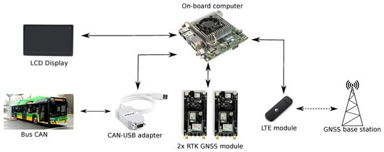
Figure 1. Hardware used in the ADAS system. The onboard computer performs all the calculations, the GNSS modules provide the position and heading of the bus, the CAN-USB adapter enables reading data from the sensors of a bus, the LTE module receives RTCM corrections over the network from the base station, and the LCD presents the system interface to the driver.

We decided to use UP Xtreme as the onboard computer, which is responsible for running the developed software and handling the data from the peripheral devices. The main tasks of this computer are processing the CAN messages, managing the data coming from the GNSS receivers, and handling the communication with the GNSS base station through the LTE module. During the docking manoeuvre, it also performs motion planning and control. The software running on this computer is described in more detail in Section 3.2. The main reason for the choice of this computer board is the x86 architecture Intel i5 CPU, which is more universal in terms of software installation than boards with ARM processors, such as Raspberry Pi or Odroid. The latter ones usually require a specific kernel and Linux version, while in the UP Xtreme case, we used the official Ubuntu 18.04 image as the operating system. What is more, the chosen board has a wide range of input voltage (12–60 V DC); thus, it can be powered directly from the bus without a need for any additional power supply units or DC–DC converters. The potential alternatives, that we considered, were the standard UP Board and UP Squared; however, their performance turned out to be significantly lower, which increased the time necessary to start the motion planner and GUI right before the manoeuvre.

The CAN-USB adapter enables the connection to the CAN bus of a vehicle and is used to read its current state. The messages that we receive using the CAN bus include information about the steering angle, the velocity of a vehicle, and the state of the pantograph (folded or raised). The first two variables are used to calculate the odometry of the bus, which is used by the motion planner in case of GNSS outage, while information about the pantograph state allowed us to confirm that the driver wants to dock to the charging station. The choice of CAN communication was dictated by the fact that all mentioned messages were already available on the CAN bus of the considered vehicle. The chosen CAN-USB adapter was produced by PEAK-System, and its advantage over different models is the galvanic isolation of the CAN connection, which assures that our system will not affect the normal operation of the bus in case of a failure.

In the role of the RTK GNSS receivers, we use two u-blox ZED-F9P modules. The first of them, called moving base, provides the position of the bus, while the second one, called rover, is used to obtain information about its yaw angle (heading). That information is critical for our application, as it is used to determine the moment of system activation and also to plan the reference path that guides the driver during the whole manoeuvre. As GNSS modules require external antennas for the proper operation, they were mounted on the bus rooftop, as presented in Figure 2. This approach ensures that the antennas have a clear view of the sky and thus receive an undisturbed signal from the satellites. The first antenna was mounted $0.2$ m ahead of the rear axle and is connected to the moving base receiver, while the second one is mounted 5 m in front of the first one and is connected to the rover module. The location of the GNSS antennas with respect to the coordinate system of the bus and synchronisation between the measurements from the GNSS and the internal bus sensors was obtained through offline calibration accomplished prior to the tests period. The calibration procedure based on optimisation techniques was the one described in [49]. Once the system was calibrated, the synchronisation between sensors is based on software timestamps.

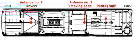
Figure 2. Mounting positions of the GNSS antennas with respect to the geometry of a bus roof. The first antenna, connected to the moving base receiver, is mounted $0.2$ m ahead of the rear axle and provides the position of a vehicle. The second one, connected to the rover module, is mounted 5 m in front of the first one and is used to calculate the bus heading.

We chose the u-blox RTK modules due to several reasons. The most important one is the possibility of operating in the moving base RTK mode, which can provide both the position and heading of a vehicle at the same time. What is more, there already exists software for easy configuration of these receivers for the Linux operating system. These receivers are also characterised by relatively low cost and are easily available, which was an additional and important factor from the commercial point of view, particularly during the pandemic times that made some electronic components hardly available. There are also other GNSS receivers available at a similar price, such as Piksi Multi from Swift Navigation and SKYTRAQ PX1122R; however, they lack the mentioned feature of heading estimation. For that reason, their usage would require manual and less accurate computation of heading angle based on the position of two antennas.

The next component is an LCD, which is simply used to present the graphical interface to the driver. It contains information about the actual position of a bus, the planned path, the desired steering angle, and path error. Its function and interface are more broadly described in Section 5. The last hardware component is an LTE module, which provides remote access and internet connectivity to the onboard computer. The module that we have selected is a generic one, and it is powered directly from the USB port of UP Extreme; thus, it starts automatically with all components. It is also used by the onboard computer to connect wirelessly to the stationary GNSS base station in order to receive the differential corrections.

The purpose of differential corrections is to improve the accuracy of positioning by reducing some errors related to GNSS signal propagation and processing. To be more specific, the corrections contain information about the tropospheric and ionospheric delays, which are caused by the Earth’s atmosphere. These delays affect the estimation of the pseudorange value, that is the distance between the receiver and each satellite, which is calculated using the time that the signal needs to travel between them.

Moreover, GNSS corrections provide also information about the satellite clock biases which also affect these measurements, as the difference between the receiver and satellite clock is used to determine the signal travel time. The GNSS base station calculates them continuously based on the signal received from each satellite and the position of its antenna that is known and fixed [50]. Estimating these errors makes it possible to calculate so-called pseudorange corrections, which can be further sent to other receivers in order to improve their pseudorange computation and thus overall accuracy. This is possible due to the fact that the influence of the atmosphere on the GNSS signal propagation is similar for all receivers that are located at a relatively short distance of several dozen kilometres from each other. What is more, corrections contain also precise information about the satellites’ orbit parameters, which are necessary to calculate their position at a given moment. They also improve the carrier phase measurements, which are based on the phase shift of the signal’s carrier wave. These measurements are more complex in terms of computations than pseudoranges and require multiple information messages from the stationary base, which are sent together with the mentioned differential corrections. In our case, all these messages are transmitted in the RTCM (Radio Technical Commission for Maritime) standard to the onboard computer, which then forwards them to the moving base receiver, thus enabling the RTK mode of localisation [50]. The source of RTCM messages that we use is the ASG-EUPOS network which provides the data from multiple reference stations located in Poland via the internet-based service.

Unfortunately, some errors cannot be reduced using RTCM data. This is especially the case for errors associated with signal multipathing and obstruction, as they depend on the actual position of a given receiver and its surroundings. The main source of this kind of error is tall buildings and trees that bounce or block the signal coming from certain satellites. For that reason, the GNSS localisation might work with less accuracy in very urbanised areas, and in some cases, such as driving through tunnels or underground parking, it does not work at all.

Another important factor that should be taken into consideration is the coverage of the GSM network in the area where the RTK GNSS is supposed to operate. This factor is usually not a problem in urban areas, but the lack of internet connection makes it impossible to receive the RTCM corrections and thus degrades the positioning precision. Fortunately, short interrupts in internet access, which can happen even in cities, are not a problem, as these corrections are usually valid for some tens of seconds. However, in the case of a longer absence of correction data, the receiver will exit the RTK mode and enter the standard FIX mode, which has the maximum static accuracy of $1.5$ m. Although it is enough to determine the approximate location of a bus, it is not sufficient for precise docking manoeuvres. For that reason, the RTCM corrections are critical for our application, and they are necessary for the system to operate correctly. In addition to the standard FIX mode, there are also two RTK modes that the GNSS receiver can be in, namely RTK FLOAT and RTK FIXED. The former is obtained when the GNSS module receives the RTCM corrections but has not managed to obtain the highest precision mode yet. The accuracy in this mode is usually at the level of tens of centimetres, which is higher than in standard FIX, but it can still vary depending on the number of visible satellites and the quality of received signals. The latter one, RTK FIXED, is the most accurate mode, and it is obtained when the receiver manages to calculate the complete navigation solution. It includes resolving the carrier phase cycle ambiguities and fixing them to the exact number of radio wavelengths between the satellites and the receiver. This ensures that the centimetre-level precision that can be maintained as long as there is no long-time interruption of RTCM data transmission, and the antennas have a clear view of the sky. All these three modes apply for both moving base and rover modules. Regardless of the current mode, the receivers use signals from multiple satellite constellations and multiple frequency bands: GPS (L1/L2), Galileo (E1/E5), and GLONASS (L1/L2). This ensures that there is always a sufficient number of visible satellites for the system to operate. What is more, it also reduces the time that is necessary to start the system after power up. In fact, the used u-blox F9P receivers obtain the standard FIX even before the whole system boots up, as they begin to calculate their position immediately after the ignition key of a bus is turned on. However, the RTK FIXED mode can be entered only after the LTE module connects to the GSM network and starts the RTCM data transmission, which additionally takes around 40–60 s to complete.

3.2. Software

In terms of software, we utilise Ubuntu 18.04 and the ROS (Robot Operating System), which is a popular set of open-source libraries and tools used in many robotic applications. Its main advantage is flexibility, as every component of our system has a dedicated package that can be started and stopped independently when required. The architecture of the developed system is presented in Figure 3. All software components are implemented as ROS nodes, which enables easy communication between different packages.

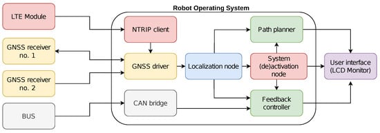
Figure 3. The architecture of the developed system. The software components were implemented as the following ROS nodes: NTRIP client, GNSS driver, CAN bridge, localisation node, system activation node, path planner, and feedback controller. The NTRIP client receives the RTCM correction using the LTE module, the GNSS driver handles the data coming from u-blox F9P receivers, the CAN bridge provides the interface for communication with the sensors mounted in the bus, the localisation node calculates the pose of a bus in relation to a charging station, the system activation node launches the motion-planning system when the bus approaches the depot, and the path planner and feedback controller generate the reference path for the driver and guide him during the docking manoeuvre.

The first component is an NTRIP (Networked Transport of RTCM via Internet Protocol) client (https://github.com/LORD-MicroStrain/ntrip_client, accessed on 3 July 2022), which is used to receive the RTCM correction using the LTE module connected to the onboard computer. As mentioned in Section 3.1, these corrections are received from an ASG-EUPOS internet-based service that provides the data from multiple GNSS base stations located in Poland. The NTRIP client task is therefore to connect to that service, receive the corrections, and then share that data with the GNSS driver.

At the same time, the GNSS driver sends the RTCM messages to the moving_base receiver so that it can enter the RTK mode. The driver is also responsible for reading the position and heading of the bus, which is sent by moving_base and rover modules accordingly. On the software level, it consists of two ROS packages that were modified for our purposes: nmea_navsat_driver (https://github.com/ros-drivers/nmea_navsat_driver, accessed on 3 July 2022) and ublox (https://github.com/KumarRobotics/ublox, accessed on 3 July 2022). The frequency of GNSS data is equal to 10 Hz for both position and heading, which is more than sufficient for the application of localisation in urban traffic.

The CAN bridge reads the current state of the bus’s internal sensors and then converts this information to ROS messages so that it can be easily used by the pose estimation and motion-planning packages. Our implementation is based on the ros_canopen (https://github.com/ros-industrial/ros_canopen, accessed on 3 July 2022) interface and uses the proprietary CAN messages provided by Solaris Bus & Coach S. A. The data obtained via the CAN interface are used to calculate the odometry of the bus and to determine the state of the pantograph.

The localisation node calculates the bus pose relative to the charger based on the data from the GNSS driver and the predetermined global pose of the charger. As the position provided by the GNSS receivers is expressed in the form of (latitude, longitude, altitude) coordinates, we perform their conversion to the UTM (Universal Transverse Mercator) system with Cartesian coordinates. For that purpose, we utilise the gps_common (https://github.com/swri-robotics/gps_umd/tree/master/gps_common, accessed on 3 July 2022) package along with the Eigen (https://eigen.tuxfamily.org/index.php?title=Main_Page, accessed on 3 July 2022) library that allows us to perform all the required transformations between the local frames of a bus and to calculate its pose in relation to a charging station. That pose is further used by the system activation node, which starts the motion-planning system right before the docking manoeuvre, as described later in this section.

The last software components are the path planner and feedback controller that generate the reference path and guide the driver to the charging station. Their principle of operation is described in more detail in Section 4.3 and Section 4.4 accordingly.

One of the important prerequisites for the ADAS supporting drivers of the public buses formulated by the bus fleet operator was that under no circumstances should the system require the driver’s attention, such as by having to set or change any parameters. This requirement was motivated by safety considerations. Therefore, the system starts automatically when the driver turns on the ignition key of the bus. After the onboard computer boots up, it starts the GNSS localisation software that from this moment is running in the background. At this time, the monitor in the driver’s cabin remains off in order not to distract the driver. When the bus approaches the selected location (during the tests at the Garbary PKM depot), at a distance of 55 m from the charger, the system launches another package that is responsible for the path planning and calculation of a steering angle. This package is launched slightly in advance so that the motion planner and graphical interface have enough time to start. In the meantime, the monitor for the driver turns on, and at the distance of 35 m, the system should be ready to use. As the position of a bus is calculated in relation to a charger, all these conditions, which are based on the distance, can be easily verified and tested. They can also be simply modified for different depots and charging stations when necessary. What is more, some additional checks are also performed in order to prevent undesired activation of a system, for example, when approaching the depot from the opposite side. From this point on, after all the packages are launched successfully, the driver can follow the displayed steering suggestions as described in more detail in Section 5. The system will turn off automatically when the bus stops under the charger and also if it detects that the driver is making another manoeuvre, such as driving the bus across the depot with no intention of docking. The system will also deactivate when the bus is more than 60 m from the charger, regardless of the manoeuvres taken by the driver. This condition is redundant; however, it assures that the system will be ready for operation during the next approach.

It is also worth mentioning that the described system is powered directly from the bus and thus can slightly affect its power demand. Thanks to the flexibility of ROS packages, which can be deactivated after the manoeuvre, we are able to run the main software only when the bus is close to the charger, and this way, we reduce the power consumption for the vast majority of the time. The Intel i5-8365UE CPU used in our version of UP Xtreme has power consumption at the level of 15 W at the maximum load, while the monitor consumes around 5.5 W. Unfortunately, all remaining components, such as the LTE module and CAN-USB adapter, are powered through a USB port and cannot be turned off automatically. This means that by reducing the CPU usage and turning off the display, we can save up to around 20 W of power. Although it seems to be insignificant when compared to the total energy consumption of the whole electric bus, which typically varies between 0.8 and 1.7 kWh per kilometre, it is simply good practice to reduce power usage whenever possible.

3.3. Performance Evaluation of the GNSS-Based Localisation System

The overall performance of GNSS was evaluated on three different routes in Poznan during the regular operation of an electric bus in city traffic. The average distance and travel time of the analysed routes are presented in Table 1. This table contains also information about the number of RTK FIXED poses registered for each sequence, which translates into the overall reliability of the system. As mentioned before, the RTK FIXED poses indicate the high-precision mode of localisation with centimetre-level accuracy, that is necessary to perform manoeuvres, such as docking to a charging station.

Table 1. The routes of the city bus recorded for the analysis of the GNSS localisation reliability and performance. RTK FIXED poses denote the high-precision mode with centimetre-level accuracy, while low-precision modes include the standard FIX and RTK FLOAT modes, and they indicate the reduced precision of the system.

Sequence (Bus Stops)	Distance	Time	Num. of Precision RTK FIXED Poses	Num. of Poses in Low Precision Modes
Dworzec Zachodni–Kacza	7.483 km	34.77 min	20,558	284
Garbary PKM–Strzeszyn	11.616 km	42.42 min	23,749	1691
Garbary PKM–Os. Dębina	9.290 km	43.93 min	25,264	1090

Based on these results, it can be stated that only a few percent ($1.36\%$, $6.65\%$, and $4.14\%$ accordingly) of registered poses are non-RTK ones. They are mainly caused by the poor visibility of the sky because of the roadside buildings and trees. However, it is worth noting that the GNSS signal was available throughout the whole sequences and there are no gaps (i.e., signal outages) in the recorded trajectories.

To facilitate statistical analysis of the GNSS localisation performance, the metric of Absolute Trajectory Error (ATE) is introduced, which is a Euclidean distance between the positions of moving_base and rover receivers corresponding in time and averaged along the route (Table 2). In order to calculate the ATE metric in this scenario, the rover coordinates were transformed to the moving_base frame by performing a translation along the longitudinal axis of the bus (in a global coordinate frame) by a vector of length $4.96$ m (distance between receivers). This vector corresponds to the exact distance between the two antennas mounted on the vehicle’s roof. This translation, however, introduces an additional error to the position of a rover, as it depends on the accuracy of heading estimation, which is also provided by the rover receiver. Unfortunately, in the real-world scenario followed in our tests, we have no possibility to measure the error of the heading estimation, as it would require either more precise ground-truth data or using an additional set of two GNSS receivers that would allow us to simply compare their measurements. Nevertheless, the results confirm that the smallest discrepancy between moving_base and rover positions was achieved for the Dworzec Zachodni–Kacza sequence, which is also characterised by the smaller number of non-RTK poses.

Table 2. Absolute Trajectory Error calculated between the poses provided by the moving_base and rover receivers. For the error calculation, the rover poses were transformed to the moving_base frame. Columns contain the sequence name and statistics (RMS, max, mean and standard deviation) of the error, respectively.

Sequence (Bus Stops)	${\mathbf{ATE}}_{\mathbf{RMS}}$	${\mathbf{ATE}}_{\mathbf{max}}$	${\mathbf{ATE}}_{\mathbf{mean}}$	${\mathbf{ATE}}_{\mathbf{std}}$
Dworzec Zachodni–Kacza	0.276 m	3.113 m	0.175 m	0.213 m
Garbary PKM–Strzeszyn	0.602 m	4.377 m	0.428 m	0.423 m
Garbary PKM–Os. Dębina	0.619 m	4.340 m	0.440 m	0.436 m

Another factor that could potentially deteriorate localisation accuracy is the mobile network coverage. This is due to the fact that our system requires constant access to the internet in order to receive the differential correction for GNSS receivers. Without these corrections, the bus positioning would be too inaccurate for our system to work properly. Fortunately, this does not apply to our case, as the GSM/LTE network was available all the time during our tests. The described routes were also plotted on the map, as presented in Figure 4A–C. This allowed us to visualise and further analyse the fragments of the trajectories, where the GNSS localisation accuracy was reduced.

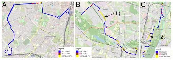
Figure 4. The recorded routes of the city bus plotted on the OpenStreetMap. RTK FIXED poses are marked with the blue line, less accurate RTK FLOAT poses are marked with a red line, and the least accurate standard GNSS poses are marked with the yellow line. Plot (A) shows the map for Dworzec Zachodni–Kacza, (B) for Garbary PKM–Strzeszyn, and (C) for Garbary PKM–Os. Dębina route.

Based on these plots, it can be seen that there are some relatively long parts of the trajectories, especially in Figure 4B,C (marked with numbers (1) and (2)) where only the standard mode is available. These parts are the narrow streets with dense canopies of trees and high-rise buildings placed along the road, as shown in Figure 5, that disturb the GNSS signal and increase the localisation error. Unfortunately, the structure of the environment significantly influences the quality of GNSS localisation, and such cases are inevitable [19,22].

Figure 5. Exemplary parts of the trajectories, where the RTK FIXED mode of GNSS was not available because of the poor sky visibility caused by buildings and trees. Image (1) presents the part of the trajectory from Figure 4B, while image (2) shows an example scene from Figure 4C.

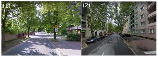
Figure 6 presents the error between moving_base and rover, calculated in an analogous manner as in Table 2, but this time only for the chosen part of the Garbary PKM–Os. Dębina trajectory. The statistical means of this error is presented in Table 3. Based on these results, it can be stated that the accuracy of GNSS-based localisation systems indeed deteriorates in these areas, as the values of an error calculated for this case are greater than for the whole sequence. Interestingly, the RMS and mean values increased by around $0.16$  m and $0.2$ m accordingly, but the standard deviation of the discussed error did not change significantly. This can suggest that positions in the non-RTK mode have a constant offset which can be caused, for example, by the multipathing of GNSS signals.

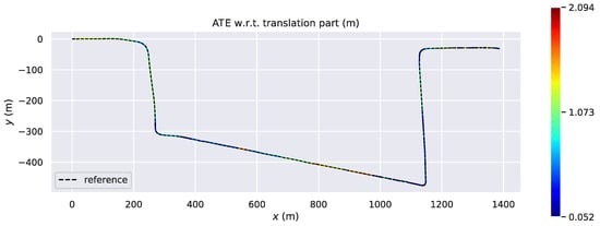
Figure 6. Absolute Trajectory Error calculated between the moving_base (reference) and rover positions. The error was calculated for the part of the Garbary PKM–Os. Dębina route where the RTK FIXED mode of GNSS was partially not available due to high buildings and trees located near the road.

Table 3. Errors between the moving_base and rover positions, calculated for the part of Garbary PKM–Os. Dębina route, where the RTK FIXED mode of GNSS was partially not available. Columns contain the sequence name, and statistics (RMS, max, mean and standard deviation of the error, respectively).

Sequence (Bus Stops)	${\mathbf{ATE}}_{\mathbf{RMS}}$	${\mathbf{ATE}}_{\mathbf{max}}$	${\mathbf{ATE}}_{\mathbf{mean}}$	${\mathbf{ATE}}_{\mathbf{std}}$
part of Garbary PKM–Os. Dębina	0.777 m	2.0943 m	0.640 m	0.439 m

However, from our point of view, the most important part of the trajectory is the area near the charging station, where the system is supposed to operate. Our ADAS can guide the bus driver to any charging station of the chosen type (in the demo application, this is the EC Ride & Charge type), as long as the geographical location of the charger in terms of the WGS84 coordinates is known. Moreover, to plan safe manoeuvres, we need to know the local map of the charger’s surroundings, which allows the ADAS to avoid static obstacles (pavement, lawns, etc.). As the considered ADAS hardware setup does not contain any external sensors to perceive the environment, we adopted the freely available OpenStreetMap data for that purpose. For the experimental evaluation presented in this article, the ADAS was configured to work with an electric charger located at the bus depot neighbouring the Garbary PKM station. Hence, we paid particular attention to the surroundings of this location when assessing the GNSS localisation accuracy. Figure 7A shows the locations of all the charging stations at this depot and the one to which the bus drivers were guided by our system (marked with a green colour). Figure 7B presents the GNSS localisation mode for the analysed area, and as can be seen, for the whole approach path, the RTK FIXED mode of the GNSS receiver is available. This means that it is possible to provide precise positioning of the bus during the entire docking manoeuvre based only on satellite navigation and without the need to use any external sensors. The main reason for that is the open space around the chargers and the lack of nearby high-rise buildings that could interfere with the satellite signals.

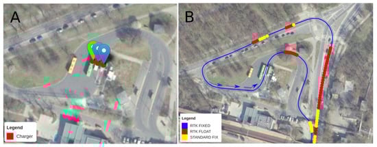
Figure 7. Position of chargers at the Garbary PKM depot (A). The green marker indicates the charger for which the developed system was set up. The GNSS localisation mode around the bus depot (B), including the approach path for which the most accurate RTK FIXED mode was available. The arrows indicate the driving direction.

4. Motion Planning and Control in ADAS for City Buses

As previously mentioned, upon approaching the charger, an underlying process ensures the activation of the ADAS motion-planning system without requiring the driver’s intervention. The motion generation subsystem, comprising a constrained path planner and a feedback controller, establishes a reference path from the bus’s current configuration to the docking station, which is considered the final configuration. Subsequently, the subsystem ensures that adhering to this path minimises errors caused by uncertainties in localisation and any driver-induced errors.

In order to ensure the feasibility of the generated path, the maximum permissible curvature and rate of curvature are deduced from the kinematic model of the bus [35]. These values are subsequently established as constraints for the planning task.

4.1. Bus Model for Low-Speed Manoeuvring

Urban buses, as shown in Figure 8, frequently perform complex low-speed manoeuvres to ensure safety and accuracy. These manoeuvres generally entail minor accelerations, resulting in negligible influence from the vehicle’s dynamics. Consequently, a kinematic model is considered suitable for adequately capturing the key properties of the vehicle’s motion throughout these manoeuvres.

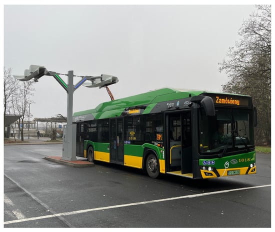
Figure 8. The electric urban bus, Solaris Urbino 12 Electric, used for the experiment in this work.

The kinematics of a rear wheel-driven car-like robot [34,51] is illustrated in Figure 9.

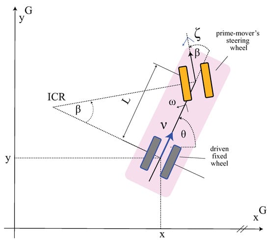
Figure 9. Car-like robot kinematics used to describe the electric bus.

The kinematic configuration of the vehicle will be represented by the vector

$$\mathit{q}\triangleq \left[\begin{array}{c}\beta \hfill \\ \overline{\mathit{q}}\hfill \end{array}\right]\in \mathcal{Q},\overline{\mathit{q}}\triangleq \left[\begin{array}{c}\theta \hfill \\ \mathit{p}\hfill \end{array}\right],\mathit{p}\triangleq \left[\begin{array}{c}x\hfill \\ y\hfill \end{array}\right]\in \mathcal{P},$$

where $\mathcal{Q}\triangleq \left[-{\beta }_m,{\beta }_m\right]\times \overline{\mathcal{Q}},{\beta }_m<\pi /2,\overline{\mathcal{Q}}=\mathbb{R}\times \mathcal{P}\subset {\mathbb{R}}^3$ is a configuration space of the vehicle kinematics.

$$\left[\begin{array}{c}\dot{\beta }\\ \dot{\theta }\\ \dot{x}\\ \dot{y}\end{array}\right]=\left[\begin{array}{cc}1& 0\\ 0& \frac{1}{L}tan\beta \\ 0& cos\theta \\ 0& sin\theta \end{array}\right]\left[\begin{array}{c}\zeta \hfill \\ v\hfill \end{array}\right]\Leftarrow \dot{\mathit{q}}=\mathit{S}\left(\mathit{q}\right)\mathit{u}.$$

(1)

Vector $\mathit{u}={\left[\zeta v\right]}^{\top }\in \mathcal{U}\subset {\mathbb{R}}^2$ is a kinematic control input comprising the steering rate $\zeta$ and longitudinal velocity v of the mid-point of the rear wheel’s axle.

The vehicle motion curvature $\kappa \triangleq \dot{\theta }/v\stackrel{\left(1\right)}{=}$$tan\beta /L$ is only dependent on the steering angle and its rate. The curvature and curvature rate limitation of the vehicle motion is imposed by ${\beta }_m<\pi /2$, hence,

$$\underset{\beta }{sup}\left|\kappa \left(\beta \right)\right|=\frac{tan{\beta }_m}{L},\underset{\beta ,\zeta }{sup}\left|\dot{\kappa }(\beta ,\zeta )\right|=\frac{{\zeta }_m}{L{cos}^2{\beta }_m}.$$

(2)

Equation (2) provides the planning module with the kinematic constraints for the task of path planning.

4.2. State Estimation

To estimate the states of the bus, a state estimation approach is employed. The states of the bus can be presented as ${\mathit{q}}_{\mathrm{CarEst}}={\left[\begin{array}{ccc}\theta & x& y\end{array}\right]}^T$; depending on the presence and delay in receiving the perception data, the state estimator follows various policies. If the localisation data indicated by ${\mathit{q}}_{\mathrm{CarLoc}}$ from the GNSS module are not present, the estimated localisation is computed by integrating (1) and applying odometry, resulting in ${\mathit{q}}_{\mathrm{CarEst}}={\mathit{q}}_{\mathrm{CarPred}}$. However, if the localisation data from GNSS are received and data are not delayed, the states are directly taken from the localisation data as ${\mathit{q}}_{\mathrm{CarEst}}={\mathit{q}}_{\mathrm{CarLoc}}$, and if the received data are delayed, a weighted sum estimator is utilised

$${\mathit{q}}_{\mathrm{CarEst}}=\mathbf{w}\odot {\mathit{q}}_{\mathrm{CarPred}}+(1-\mathbf{w})\odot {\mathit{q}}_{\mathrm{CarLoc}}$$

(3)

where ⊙ denotes the element-wise (Hadamard) product, and $\mathbf{w}$ is a vector containing the weight parameters for each component. Here $\mathbf{w}=[w_{\mathrm{theta}},w_{\mathrm{pos}},w_{\mathrm{pos}}]$ are the weight parameters for the theta and position components, respectively.

4.3. Path Planning in Restricted Areas

In the prototype ADAS solution, thanks to the specific properties of the docking manoeuvre, path planning was facilitated by analytical (geometrical) relations, and for more difficult manoeuvres, the state lattices approach [52] was utilised. This was made possible by formulating the path-planning problem as a graph search problem where a predefined set of path primitives is expanding recursively until the optimum path is found [34]. This planner samples from a finite set of motion primitives that could lead to the generation of a suboptimal path, especially in terms of steering wheel movement, which was difficult for the human driver to follow. Therefore, for the ADAS variant evaluated by MPK Poznań, a more general approach to path planning under various constraints was desired. The method for path planning, including monotonic docking or parking manoeuvres, should take into account kinematic constraints while not being limited to the use of specific curves. Such a method was implemented based on the non-linear optimisation of coefficients of a 7th-degree polynomial defined as the reference path. The path-planning objective function is subjected to the initial and final configuration of the bus, the kinematic constraints, which are defined as curvature and rate of curvature (2), and the constraints resulting from obstacles. The advent of efficient interior point optimisation methods has enabled a tractable solution to large-scale linear and non-linear programming problems. Considering this fact, our planner is implemented taking advantage of the CasADi software [53] that utilises the IPOPT (Interior Point OPTimizer) [54] library for the large-scale non-linear optimisation of continuous systems to solve the optimisation problem in path planning.

As the planner must provide an obstacle-free path, it needs to consider a local map of the environment around the electric charger’s site. Although our earlier approach to path planning used a local grid map of the environment, the new variant avoids the direct use of an occupancy grid because of two reasons. First, the version of ADAS implemented for the presented evaluation does not use any external sensors; thus, it cannot build an occupancy map online. Second, a detailed (high-resolution) occupancy grid made path planning slower. Hence, we take advantage of the new formulation of the planning problem as optimisation with equality and inequality constraints, and we transform a local map of the scene around the charger, together with the bus and the charger’s configurations, into a set of constraints for optimisation. These inequality constraints define the allowed area of motion for the bus while executing the manoeuvre. As our ADAS cannot build its own map of the environment, it leverages the available internet access and accurate position information from RTK GNSS to obtain the layout of objects around the charger from the OpenStreetMaps free service.

The downloaded local map is then used to generate automatically multiply bounding boxes (Figure 10) using Algorithm 1. These boxes provide positional inequality constraints of the control points placed on the polynomial.

Algorithm 1: Generating bounding rectangles.

Input: initial and final configurations: $P_0(x_0,y_0,{\theta }_0)$ and $P_F(x_F,y_F,{\theta }_F)$. functionCalculateWeight($p_1,p_2$)     $h\leftarrow \sqrt{{(x_{p_2}-x_{p_1})}^2+{(y_{p_2}-y_{p_1})}^2}$     while obstacle free do         Expand the rectangle normal to the line segments h by $\Delta w$. az         $w\leftarrow w+\Delta w$     end while     return $h,w$ end function Calculate $y=m_{0}x+b_0$ and $y=m_{F}x+b_F$ lines along $P_0$ and $P_F$. $P_c\leftarrow (x_c,y_c)$             ▹ Calculate intersection point of two lines $re{c}_1(h_1,w_1)\leftarrow CalculateWeight(P_0,P_c)$ $re{c}_3(h_3,w_3)\leftarrow CalculateWeight(P_c,P_F)$ $re{c}_2(h_2,w_2)\leftarrow CalculateWeight(P_c+w_1/2,P_c-w_1/2)$ Output: The height h and weight w of each rectangles $rec1,rec2,rec3$.

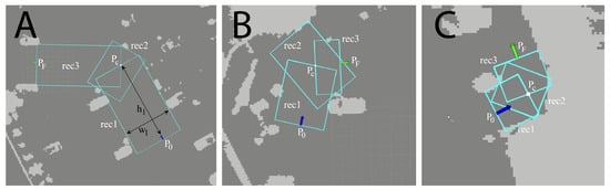
Figure 10. Bounding boxes are generated to provide the planner with a safe and obstacle-free tunnel interpreted as positional inequality containers; in this figure, (A–C) present different locations subject to path planning. The blue arrow denotes the initial configuration of the bus while the green one charger configuration.

This algorithm takes in at input the current and final configuration of the bus $P_0(x_0,y_0,{\theta }_1)$ and $P_F(x_F,y_F,{\theta }_F)$, and then, after computing slopes of lines along with these two configurations, calculates the intersecting point $P_c$. Two line segments, $(P_0,P_c)$ and $(P_c,P_F)$, are generated. By expanding the intersection configuration, an additional line segment is generated toward the final and initial configuration, which guarantees the coverage between two other rectangles. While obstacle free, it then iterates over all cells of the grid map perpendicularly to these three lines.

Given a set of control points $P=p_0,p_1,\dots ,p_m$, where $p_0$ is the current configuration of the bus and $p_m$ is the final configuration, the objective is to find a polynomial function $f\left(x\right)=c_0+c_{1}x+c_2{x}^2+...+c_n{x}^n$ that passes through all the control points. The optimisation problem is subject to a number of constraints, including the initial and final configuration of the path, as well as constraints on the control points, the curvature and rate of curvature of the path, and the position of the path at each control point. The optimisation problem is presented by

$$\begin{array}{cc}\hfill \underset{c_0,c_1,\dots ,c_n}{\mathrm{minimise}}& \sum _{i=1}^m{f}_i^2\mathrm{subject}\mathrm{to}\hfill \\ \hfill & f\left(x_j\right)=y_j\forall j\in 1,2,\dots ,m,\hfill \\ \hfill & f\left(x_0\right)=p_0,f\left(x_m\right)=p_m,\hfill \\ \hfill & \left|\kappa \left(f\left(x_i\right)\right)\right|\stackrel{\left(2\right)}{\le }{\kappa }_{\max }\forall i\in 1,2,\dots ,m,\hfill \\ \hfill & \left|\dot{\kappa }\left(f\left(x_i\right)\right)\right|\stackrel{\left(2\right)}{\le }{\dot{\kappa }}_{\max }\forall i\in 1,2,\dots ,m,\hfill \\ \hfill & y_i\mathrm{bounded}\mathrm{inside}\mathrm{rectangles}\mathrm{from}\mathrm{Algorithm}1,\forall i\in 1,2,\dots ,m,\hfill \end{array}$$

where $c_0,c_1,\dots ,c_n$ are the coefficients of the polynomial, $f\left(x\right)$ is the polynomial function, $x_i$ and $y_i$ are the i-th control point coordinates, m is the total number of control points, and $f_i$ is the distance between the i-th control point and the polynomial evaluated at $x_i$. The objective function minimises the sum of the squares of the distances between each control point and the polynomial, which is subject to the constraints that the polynomial passes through each control point and satisfies the specified constraints at each control point.

The first constraint ensures that the polynomial function passes through the starting points and endpoints. The second constraint limits the maximum curvature of the path to ${\kappa }_{max}$ to ensure that the path is feasible for the kinematics of the bus.

The optimisation problem can be solved using the Interior Point Optimiser [54], which is a type of non-linear programming algorithm that can handle inequality constraints. The algorithm iteratively updates the solution until a convergence criterion is met.

4.4. Feedback Control

Following [34], a feedback control law is formulated to provide motion corrections based on the presented vehicle-body kinematics (1) utilising a Vector-Field-Orientation (VFO) [36] controller. The controller takes the form

$${\varphi }_0\left(\overline{\mathit{q}}\right)=\left[\begin{array}{c}{\varphi }_{\omega 0}\left(\overline{\mathit{q}}\right)\hfill \\ {\varphi }_{v0}\left(\overline{\mathit{q}}\right)\hfill \end{array}\right]\triangleq \left[\begin{array}{c}{h}_{\theta }\left(\overline{\mathit{q}}\right)\\ h_x\left(\mathit{p}\right)c\theta +h_y\left(\mathit{p}\right)s\theta \end{array}\right],$$

(4)

resulting in the convergence vector field components

$$h_{\theta }\triangleq k_a\underset{e_a}{\underbrace{\left({\theta }_a-\theta \right)}}+{\dot{\theta }}_a,\left[\begin{array}{c}{h}_x\hfill \\ h_y\hfill \end{array}\right]\triangleq k_{p}F\left(\mathit{p}\right)\vartheta +v_d\mathit{R}\vartheta ,$$

(5)

where $v_d>0$ represents the absolute value of a reference longitudinal velocity along the path, $k_a>k_p>0$ are design parameters, whose values were determined by taking a baseline value from the simulation and tuned during the experiments in the field, and $\mathit{R}=\left[\begin{array}{cc}0& 1\\ -1& 0\end{array}\right]$ is a rotation operator of the $-\pi /2$ angle, while

$${\theta }_a\triangleq Atan2\mathrm{c}\left({\zeta }_d{h}_y,{\zeta }_d{h}_x\right)\in \mathbb{R},\vartheta \triangleq -\nabla F/\parallel \nabla F\parallel$$

(6)

can be defined as the auxiliary orientation and the unit vector of a negative gradient of the function $F\left(\mathit{p}\right)$, respectively. Having the outer-loop control function (4), one introduces the computed vehicle-body velocities

$${\mathit{u}}_{0c}={\left[{\omega }_{0c}{v}_{0c}\right]}^{\top }\triangleq {\varphi }_0\left(\overline{\mathit{q}}\right),$$

(7)

where ${\kappa }_{0c}={\omega }_{0c}/v_{0c}$ is determined uniquely as an instantaneous motion curvature and a corresponding computed steering angle

$${\beta }_c\left({\varphi }_0\left(\overline{\mathit{q}}\right)\right)\triangleq arctan\left(L{\kappa }_{0c}\right)\stackrel{\left(7\right)}{=}arctan\left(L\frac{{\varphi }_{\omega 0}\left(\overline{\mathit{q}}\right)}{{\varphi }_{v0}\left(\overline{\mathit{q}}\right)}\right),$$

(8)

with ${\varphi }_{\omega 0}\left(\overline{\mathit{q}}\right)$ and ${\varphi }_{v0}\left(\overline{\mathit{q}}\right)$ resulting from (4). Following the work [37], control signals (7) and steering angle (8) provide the control inputs ${\mathit{u}}_c\left(\overline{\mathit{q}}\right)={\left[{\zeta }_c\left(\overline{\mathit{q}}\right)v_c\left(\overline{\mathit{q}}\right)\right]}^{\top }$. Since our ADAS is providing a steering angle indicator to the human driver, it only utilises (8) in a saturated form

$${\beta }_d\left({\varphi }_0\left(\overline{\mathit{q}}\right)\right)\triangleq sat\left({\beta }_c\left({\varphi }_0\left(\overline{\mathit{q}}\right)\right),{\beta }_m\right),$$

(9)

where $sat\left(\alpha ,{\alpha }_m\right)\triangleq min\left\{\left|\alpha \right|,{\alpha }_m\right\}·sign\left(\alpha \right)$ is a conventional saturation function, while ${\beta }_m$ corresponds to the constraint imposed by the admissible configuration set.

As illustrated in Figure 11, the desired steering angle ${\beta }_d$ and the actual steering angle $\beta$ are visualised for the human driver through the ADAS human–machine interface. The human driver then is expected to follow the steering angle indicator to track the generated path. Manoeuvres leading to the displacement of the bus to the reference path are corrected via the Vector-Field-Orientation (VFO) [36] controller to a defined threshold. The steering suggestions displayed to the driver are the ones corrected by the VFO algorithm; thus, they take into account any inaccuracies of path following. However, a large displacement from the reference path cannot be corrected by VFO and can lead to re-planning the path from the current configuration of the bus.

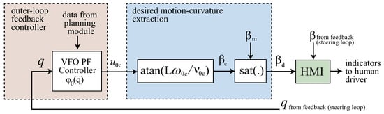
Figure 11. Block scheme explaining connections between the control module and the interface subsystem.

5. Human-Machine Interface in ADAS

A 10-inch, 1920 × 1200 pixel resolution (Full HD) dedicated monitor with viewing angles of 178° from Beetronics has been mounted on the driver’s dashboard.

This monitor is connected to the ADAS computer via an HDMI cable and automatically powered on when approaching the charger position, displaying the HMI. The HMI consists of a 3D model of the bus together with the reference path shown to the driver for a better understanding of the complete manoeuvre and a set of colour bars that indicate the steering angles and suggest the steering wheel operation.

In order to follow the reference path, the driver is provided with a visual configuration of the bus consisting of the actual and reference steering angle. The actual steering angle bar is composed of three different colours depending on the error of the steering angle. When following the reference angle closely, the bar is drawn in green, while the bigger the error, the colour is changed to orange and then to red.

The remaining distance bar indicates how far the pantograph is to its correct position under the charger, and the complete scheme is shown in Figure 12.

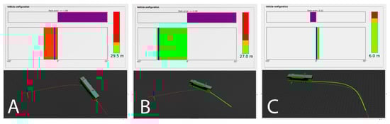
Figure 12. Human–machineinterface in ADAS system. The top purple coloured bar indicates the path error: that is, the displacement of the bus’s guidance point from the reference path. The main bar provides steering guidance, consisting of a solid blue line visualising the desired steering angle, and a coloured-filled area indicating the actual steering angle. The colour of the bar is sensitive to the value of the steering error: an acceptable error is shown by green colour, while the bigger the error becomes, the colour changes to orange and red. The vertical bar placed on the right side of the window indicates the remaining distance to the charger; at zero, the pantograph is located exactly below the charger. (A): At this state, the centre of the rear axis of the bus (guidance point) is more than one metre away from the reference path, and the driver must turn the steering wheel to the right to align the actual steering with the blue line indicating the desired steering angle. The red portion of the right vertical bar shows the bus still has to proceed further to reach the charger. (B): The actual and reference steering is aligned with acceptable precision; however, the guidance point is still more than one metre away from the reference path. From the vertical bar, it can be seen that the bus is closer to the goal pose compared to the image on the left. (C): At this state, the reference steering angle is shown around zero, and the actual steering angle is shown around the same value. As the driver follows the guidance and keeps the wheels straight, the bus remains on the reference path and finally reaches the goal pose.

Early field tests revealed that by following the guidance bar of steering on the HMI graphical interface, the indicator for the remaining distance from the pantograph to the charger was neglected, as the driver keeps minimising the error of steering during the whole manoeuvre. This led to passing the charger’s head position and stopping the bus after the charger.

Hence, a sound indicator was added to the system to overcome this problem. A short beep indicates that the bus is in the vicinity of the charger, the smaller the distance to the charger, the longer the beeps produced by the sound indicator, also known as dashed beeps, which eventually transform into a continuous sound signal by arriving at the charger’s head position.

Taking advantage of hearing and visual senses, the driver can receive the steering suggestions and react to both signals, eventually following the steering guidance bar by turning the driving wheel and stopping the bus at the exact location of the charger.

6. Experimental Results

6.1. Environment and Scenario

The data that were used for the evaluation were collected during the normal operation of a bus in the city of Poznan. It includes the sequences from two different bus lines: no. 160 and 176. The system starts up automatically when the bus approaches the charging stations requiring no driver input to be enabled, and then steering suggestions are shown to the driver using the HMI monitor in the cabin. Thanks to the fully automatic solution, it was possible to remotely record the necessary data across multiple days whenever the bus was approaching the charging station. For the evaluation, we chose the recorded approaches from a single bus in December 2022 during the usual operating hours from 4:30 A.M. to 11:00 P.M., resulting in 50 sequences of attempted docking to the selected charging station. December was chosen as the most challenging month due to the poor weather conditions (i.e., snow, short sunlight hours, cloudy sky, smog) that affect both driver’s perception and GNSS signal strength. We expect that these conditions are the most challenging to the GNSS localisation accuracy in the entire period of the experiment.

All the data were recorded to the hard drive of the onboard computer in the form of a .bag file, which is a format used in ROS for storing different message types. It also offers multiple tools for the analysis and visualisation of recorded sequences and also makes it possible to replay the data for simulation purposes. In our case, each .bag file corresponds to a single docking approach so that we can process them individually and verify whether they are complete and contain the data that are necessary for evaluation. The most important data from this perspective are the actual position of a bus and the reference path, generated by the motion planner, as it is necessary to calculate the path error and also to determine whether the manoeuvre was successful. For validation and debugging purposes, we also recorded the GNSS data, as it allows us to confirm the RTK mode of localisation. Each recorded sequence takes between 30 and 70 s and contains the following messages types: raw data from two GNSS receivers (10 Hz), poses of a bus calculated based on GNSS data (10 Hz), processed CAN messages (100 Hz), the output of a bus state estimator (40 Hz), the output of a feedback controller (40 Hz), and a single reference path generated individually for each manoeuvre.

6.2. Results of the Docking Experiments

First, we analysed the path deviation between a real trajectory of the bus and the path planned by our system. Table 4 presents the numerical values of that deviation for 50 sequences, where the bus stopped under the charger for which our system is operating. The deviation was calculated as Absolute Trajectory Error, where in this scenario, ATE is the Euclidean distance between the real and planned trajectory computed for each corresponding pose, and it is averaged over the entire trajectory. This type of error measures both the inaccuracy of the system when the driver follows the system’s guidance and the tracking error when drivers ignore the system’s suggestions.

Table 4. Absolute Trajectory Error calculated between the reference (planned) and real paths for the docking manoeuvre of a bus. Columns contain the sequence number and statistics (RMS, max, mean and standard deviation) of the error, respectively.

Seq.	${\mathbf{ATE}}_{\mathbf{RMS}}$	${\mathbf{ATE}}_{\mathbf{max}}$	${\mathbf{ATE}}_{\mathbf{mean}}$	${\mathbf{ATE}}_{\mathbf{std}}$
1	0.680 m	1.585 m	0.558 m	0.390 m
2	0.423 m	0.668 m	0.391 m	0.159 m
3	0.649 m	1.600 m	0.527 m	0.379 m
4	1.370 m	3.193 m	0.985 m	0.953 m
5	0.866 m	2.247 m	0.626 m	0.599 m
6	0.765 m	1.966 m	0.575 m	0.504 m
7	0.766 m	1.967 m	0.599 m	0.479 m
8	1.270 m	3.141 m	0.872 m	0.923 m
9	0.535 m	1.084 m	0.471 m	0.254 m
10	1.001 m	2.562 m	0.716 m	0.700 m
11	0.910 m	2.294 m	0.679 m	0.605 m
12	0.808 m	2.068 m	0.618 m	0.520 m
13	0.688 m	1.745 m	0.536 m	0.432 m
14	0.892 m	2.282 m	0.662 m	0.597 m
15	0.543 m	1.347 m	0.478 m	0.258 m
16	1.501 m	3.584 m	1.028 m	1.093 m
17	0.574 m	1.152 m	0.503 m	0.277 m
18	0.875 m	2.257 m	0.638 m	0.599 m
19	0.626 m	1.295 m	0.543 m	0.311 m
20	0.923 m	2.281 m	0.708 m	0.592 m
21	0.525 m	1.211 m	0.473 m	0.229 m
22	0.547 m	1.267 m	0.479 m	0.265 m
23	0.644 m	2.166 m	0.535 m	0.358 m
24	0.746 m	1.820 m	0.593 m	0.452 m
25	0.529 m	1.075 m	0.473 m	0.237 m
26	0.944 m	2.423 m	0.684 m	0.651 m
27	0.561 m	1.238 m	0.510 m	0.234 m
28	0.560 m	1.354 m	0.472 m	0.303 m
29	0.889 m	2.301 m	0.649 m	0.606 m
30	0.600 m	1.317 m	0.517 m	0.306 m
31	1.135 m	2.863 m	0.790 m	0.815 m
32	0.506 m	1.009 m	0.449 m	0.234 m
33	0.612 m	1.500 m	0.504 m	0.347 m
34	0.858 m	2.224 m	0.646 m	0.565 m
35	0.987 m	2.506 m	0.721 m	0.675 m
36	0.725 m	1.861 m	0.567 m	0.453 m
37	0.895 m	3.138 m	0.671 m	0.593 m
38	1.192 m	4.372 m	0.781 m	0.901 m
39	0.897 m	3.093 m	0.655 m	0.613 m
40	0.623 m	1.560 m	0.504 m	0.368 m
41	0.556 m	1.319 m	0.476 m	0.287 m
42	0.577 m	1.381 m	0.491 m	0.303 m
43	0.537 m	1.123 m	0.479 m	0.241 m
44	0.603 m	1.342 m	0.520 m	0.304 m
45	1.140 m	2.861 m	0.859 m	0.749 m
46	1.420 m	3.466 m	0.960 m	1.047 m
47	1.169 m	2.896 m	0.811 m	0.842 m
48	1.570 m	5.257 m	1.014 m	1.199 m
49	1.000 m	2.560 m	0.708 m	0.707 m
50	0.587 m	1.299 m	0.506 m	0.297 m

As can be noted, the error values differ significantly across multiple sequences. However, for all of them, the displacement value was small enough not to cause the re-planning of a reference trajectory. This means that only a single path was generated by the motion planner for each of the considered trials, which has an important advantage in terms of computational complexity. Unfortunately, the drawback of this approach is that in case the driver does not follow the system’s suggestions from the very beginning, the RMS value of error will typically stay in the range of $0.5$–$1.0$ m. This is the case for almost all the results in the considered table. However, all of these 50 sequences were successful, which naturally indicates that many various paths can be considered correct, as long as the final part of the trajectory leads to the charger’s head. From this perspective, the more important indicator of the system performance seems to be the displacement value at the very end of a manoeuvre, as described in Section 6.3.

The examples of two trajectories, recorded during the docking manoeuvre, are presented in Figure 13 and Figure 14. What we observe is that the accumulated tracking error for all 50 sequences has a peak from around 25 m to the charger. At that distance, the drivers preferred to follow a different path (shorter to target) compared to the one proposed by the planning system (putting the bus straight to the target as soon as possible). Unfortunately, as the system was working in the background, we are neither able to confirm nor deny if there are different preferences among the tested drivers. Moreover, it might be the case that the drivers are concerned about the charging manoeuvre when they are closer to the desired charging location compared to the planning path window. Naturally, the tracking error between the taken path and the path proposed by the system is slowly converging to zero as both paths approach the desired charging location.

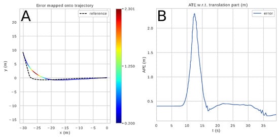
Figure 13. Reference and real path of the bus generated for the bus approach to the charging station. The point (0, 0) is the charger location (A). The Absolute Trajectory Error between the reference and real trajectory over time (B). Plots present the results for sequence 42.

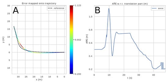
Figure 14. Reference and real path of the bus, generated for the bus approach to the charging station. The point (0, 0) is the charger location (A). The Absolute Trajectory Error between the reference and real trajectory over time (B). Plots present the results for sequence 12.

6.3. Accuracy of the Docking Manoeuvres

The goal of the docking is to successfully connect and charge the battery of the electric bus. In Poznan, the EC Ride & Charge setup (https://ec-e.pl/produkty/ride-and-charge/, accessed on 8 April 2023) is used. Based on the documentation [55], the system can properly dock when the pantograph positioning error does not exceed the lateral error of 0.45 m and longitudinal error of 0.75 m with respect to a perfect charging location. The errors obtained for our docking scenarios are presented in Table 5. Among the 50 experiments, all of them resulted in a final position that had a lower error compared to the requirements put by the charging system indicating that all of them could be used to successfully charge the battery. However, as it is a mechanical guidance system, it might wear if the docking error is relatively large compared to the desired position. The maximum lateral error for our docking scenario did not exceed 0.185 m, which is roughly 41% of the maximal error accepted by the charging station. All of these docking attempts were successful with the lateral position margin wide enough for the used electric charger technology. Moreover, the obtained errors would still allow for a successful docking with other chargers having lower docking tolerances, e.g., Shunk chargers used in [3], making the proposed solution viable for a wide range of charger–pantograph choices.

Table 5. Errors of bus position under the charger, at the end of the docking manoeuvre: ${\mathrm{x}}_{\mathrm{err}}$ denotes the longitudinal error, along the length of a bus, while ${\mathrm{y}}_{\mathrm{err}}$ denotes the lateral error spanning the width of a bus body.

Seq.	${\mathbf{x}}_{\mathbf{err}}$	${\mathbf{y}}_{\mathbf{err}}$
1	0.039 m	0.053 m
2	−0.009 m	−0.028 m
3	−0.373 m	0.178 m
4	0.043 m	0.042 m
5	−0.403 m	−0.042 m
6	0.369 m	0.028 m
7	0.262 m	0.095 m
8	0.154 m	0.161 m
9	−0.099 m	−0.053 m
10	−0.146 m	−0.035 m
11	0.476 m	0.060 m
12	−0.013 m	0.031 m
13	0.116 m	−0.038 m
14	0.390 m	−0.024 m
15	0.026 m	−0.063 m
16	0.150 m	−0.073 m
17	0.412 m	0.021 m
18	−0.223 m	−0.091 m
19	0.189 m	0.077 m
20	0.051 m	−0.028 m
21	0.167 m	−0.017 m
22	0.120 m	0.000 m
23	0.021 m	−0.003 m
24	0.180 m	0.000 m
25	0.056 m	−0.087 m
26	0.356 m	0.011 m
27	0.335 m	0.014 m
28	−0.051 m	−0.119 m
29	0.176 m	−0.038 m
30	0.429 m	0.028 m
31	−0.051 m	−0.119 m
32	0.013 m	−0.080 m
33	0.086 m	−0.112 m
34	0.167 m	0.179 m
35	−0.335 m	−0.063 m
36	−0.124 m	−0.039 m
37	0.064 m	−0.059 m
38	−0.013 m	0.031 m
39	0.163 m	0.042 m
40	0.322 m	0.046 m
41	0.077 m	−0.091 m
42	0.017 m	−0.042 m
43	0.468 m	0.081 m
44	−0.189 m	0.070 m
45	0.017 m	0.007 m
46	−0.210 m	−0.025 m
47	−0.322 m	0.052 m
48	−0.236 m	−0.060 m
49	−0.004 m	−0.185 m
50	0.056 m	0.109 m

The errors for all of the docking runs are reported in Table 5 with statistical means presented in Table 6.

Table 6. The mean and standard deviation values of a localisation error of a bus position under the charger at the end of the docking manoeuvre. The values were calculated based on the data from Table 5.

${\mathbf{x}}_{\mathbf{mean}}$	${\mathbf{x}}_{\mathbf{std}}$	${\mathbf{y}}_{\mathbf{mean}}$	${\mathbf{y}}_{\mathbf{std}}$
0.063 m	0.219 m	−0.004 m	0.077 m

Figure 15 presents the relationship between the trajectory error and the distance from the charger. As can be noted, the peak value of the error occurs for the distance between 25 and 30 m from the charging station. Based on this plot, it can be concluded that the drivers performed the manoeuvre in a slightly different way than planned by our system at that distance. The reason for this might be that the proposed path was less convenient or required a change in the driver’s habits.

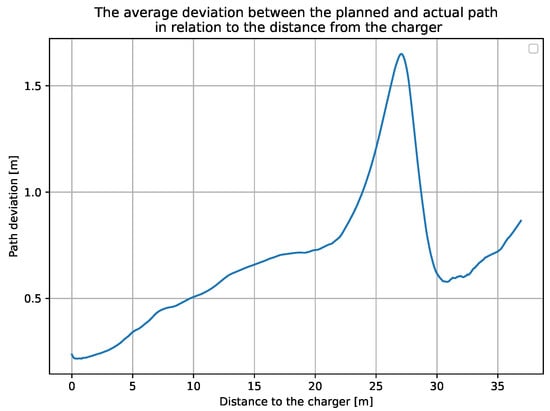
Figure 15. The average deviation between the planned and actual path in relation to the distance from the charger. The average value was calculated based on all 50 sequences.

6.4. Failure Modes

The system evaluation results in the previous section were presented for the 50 charging attempts, which were selected from the attempts made by the bus drivers during the period of data acquisition in December 2022. The bus depot area contained three chargers located in close vicinity to each other (Figure 7). Since the end-user, for safety reasons, requested a fully automated procedure to support docking to the chargers, without the driver having to interfere with the ADAS system, e.g., by selecting options via buttons, a scenario was assumed whereby the bus drivers should use charger number one, which is located closest to the open space of the bus depot. However, in practice, the drivers also used the other two, for example, if charger number one was just occupied by another bus. Although the resolution of the RTK GNSS localisation system makes it possible to distinguish these three chargers by their location, it is impossible to tell which charger the driver wants to dock to when he/she starts the manoeuvre, as in fact, the initial parts of the trajectories are almost the same for all these chargers located close to each other and in one line. In addition, the driver can change his/her decision about which charger he/she wants to dock during the manoeuvre if an unexpected obstacle arises, such as a person passing through the depot area. Whereas it would be possible to ask the drivers to select the charger they want to dock to using the HMI, e.g., with a touchscreen, a dynamic selection of the charging station was concluded too confusing to the drivers due to a rapid change in the recommended driving cues. Therefore, we had to consider all attempts to dock to another charger than the one selected in the scenario as failures of the ADAS solution. An example of a case when the driver was approaching a different charger than our system planned is presented in Figure 16. This demonstrates a major drawback of the presented approach, as a completely passive system is not able to tell if the driver wants to approach the left or right charging station if they are mounted on the same pylon.

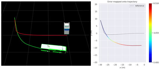
Figure 16. The visualisation of the docking manoeuvre trajectory for the case when the driver approaches a different charger than assumed by our system.

As can be noted, regardless of the charger selected by the driver, the beginning of the trajectory starts approximately at the same position. Unfortunately, this makes it impossible for our system to reliably predict which charging station the driver is going to approach.

7. Conclusions

This paper presented the results of a long-term study of an ADAS system designed to assist drivers of electric city buses in the task of docking to charging stations at bus stops or depots. The system we proposed is an extension of our earlier work on the problems of ADAS for city buses but is a cost-accessible version optimised for use in any bus, not just newly manufactured ones. The actual system has been proven in the operational environment, which corresponds to Technology Readiness Level 9 (TRL 9).

The presented results indicate that the localisation solution with two GNSS receivers and RTK correction from a service publicly available via the Internet is sufficiently precise for the considered task. Positioning errors of the bus with the pantograph raised (during charging) were minor, and failed manoeuvres to reach the charger were caused in all recorded cases by the driver’s failure to follow the ADAS suggestions. Therefore, we conclude that the RTK-GNSS technology is mature and reliable enough to support precise manoeuvres of electric buses as long as the considered scenario prevents the bus from operating in degraded GNSS signal zones, such as the vicinity of high-rise buildings or dense tree canopies. Whereas the interference of the satellite signals with the environment has to be considered as a potential cause of degraded accuracy, the distribution of RTCM corrections using the commonly available GSM network and LTE technology was reliable regardless of the environmental characteristics and weather. This observation suggests that resources available via the Internet, such as OpenStreetMap, can be used to support urban transportation in real time, increasing the autonomy of vehicles and decreasing the costs of deployment.

In the near future, the development of the proposed ADAS for docking manoeuvres of electric buses should focus on an improved user interface integrating the HMI within the driver’s dashboard. This is, however, out of the scope of the project aimed at retrofitting the ADAS to the existing fleet of buses, as it requires changes to the bus design being made at the production stage. Further development can include the integration of affordable LiDAR sensors for environment monitoring and re-planning of the trajectories while approaching the charging station in response to emerging obstacles, including dynamic ones.

References

- Vilppo, O.; Markkula, J. Feasibility of Electric Buses in Public Transport. World Electr. Veh. J. 2015, 7, 357–365. [Google Scholar] [CrossRef]
- Correa, G.; Muñoz, P.; Rodriguez, C. A comparative energy and environmental analysis of a diesel, hybrid, hydrogen and electric urban bus. Energy 2019, 187, 115906. [Google Scholar] [CrossRef]
- Michalek, M.M.; Gawron, T.; Nowicki, M.; Skrzypczynski, P. Precise Docking at Charging Stations for Large-Capacity Vehicles: An Advanced Driver-Assistance System for Drivers of Electric Urban Buses. IEEE Veh. Technol. Mag. 2021, 16, 57–65. [Google Scholar] [CrossRef]
- Shuttleworth, J. SAE Standards News: J3016 Automated-Driving Graphic Update. Available online: https://www.sae.org/news/2019/01/sae-updates-j3016-automated-driving-graphic (accessed on 4 April 2023).
- Nowak, T.; Nowicki, M.R.; Skrzypczyński, P. Vision-based positioning of electric buses for assisted docking to charging stations. Int. J. Appl. Math. Comput. Sci. 2022, 32, 583–599. [Google Scholar]
- Jiang, L.; Diao, X.; Zhang, Y.; Zhang, J.; Li, T. Review of the Charging Safety and Charging Safety Protection of Electric Vehicles. World Electr. Veh. J. 2021, 12, 184. [Google Scholar] [CrossRef]
- Deng, R.; Liu, Y.; Chen, W.; Liang, H. A Survey on Electric Buses: Energy Storage, Power Management, and Charging Scheduling. IEEE Trans. Intell. Transp. Syst. 2021, 22, 9–22. [Google Scholar] [CrossRef]
- Ma, T.Y.; Fang, Y. Survey of charging management and infrastructure planning for electrified demand-responsive transport systems: Methodologies and recent developments. Eur. Transp. Res. Rev. 2022, 14, 1866–8887. [Google Scholar] [CrossRef]
- Iclodean, C.; Cordos, N.; Varga, B.O. Autonomous Shuttle Bus for Public Transportation: A Review. Energies 2020, 13, 2917. [Google Scholar] [CrossRef]
- Bengler, K.; Dietmayer, K.; Farber, B.; Maurer, M.; Stiller, C.; Winner, H. Three Decades of Driver Assistance Systems: Review and Future Perspectives. IEEE Intell. Transp. Syst. Mag. 2014, 6, 6–22. [Google Scholar] [CrossRef]
- Ye, W.; Xu, Y.; Zhou, F.; Shi, X.; Ye, Z. Investigation of Bus Drivers’ Reaction to ADAS Warning System: Application of the Gaussian Mixed Model. Sustainability 2021, 13, 8759. [Google Scholar] [CrossRef]
- Chada, S.K.; Thomas, J.M.; Görges, D.; Ebert, A.; Teutsch, R. Ecological Adaptive Cruise Control for City Buses based on Hybrid Model Predictive Control using PnG and Traffic Light Information. In Proceedings of the IEEE Vehicle Power and Propulsion Conference (VPPC), Gijon, Spain, 25–28 October 2021; pp. 1–7. [Google Scholar]
- Yang, D.; Seo, S.W. Traffic Light Detection using Attention-Guided Continuous Conditional Random Fields. In Proceedings of the International Conference on Electronics, Information, and Communication (ICEIC), Jeju, Republic of Korea, 6–9 February 2022; pp. 1–3. [Google Scholar]
- Roszyk, K.; Nowicki, M.R.; Skrzypczyński, P. Adopting the YOLOv4 Architecture for Low-Latency Multispectral Pedestrian Detection in Autonomous Driving. Sensors 2022, 22, 1082. [Google Scholar] [CrossRef]
- Pérez, J.; Nashashibi, F.; Lefaudeux, B.; Resende, P.; Pollard, E. Autonomous Docking Based on Infrared System for Electric Vehicle Charging in Urban Areas. Sensors 2013, 13, 2645–2663. [Google Scholar] [CrossRef] [PubMed]
- Al-Saadi, M.; Mathes, M.; Käsgen, J.; Robert, K.; Mayrock, M.; Mierlo, J.V.; Berecibar, M. Optimization and Analysis of Electric Vehicle Operation with Fast-Charging Technologies. World Electr. Veh. J. 2022, 13, 20. [Google Scholar] [CrossRef]
- Petrov, P.; Boussard, C.; Ammoun, S.; Nashashibi, F. A hybrid control for automatic docking of electric vehicles for recharging. In Proceedings of the IEEE International Conference on Robotics and Automation, Saint Paul, MN, USA, 14–18 May 2012; pp. 2966–2971. [Google Scholar]
- Miseikis, J.; Ruther, M.; Walzel, B.; Hirz, M.; Brunner, H. 3D Vision Guided Robotic Charging Station for Electric and Plug-in Hybrid Vehicles. arXiv 2017, arXiv:1703.05381. [Google Scholar]
- Gu, Y.; Hsu, L.T.; Kamijo, S. Towards lane-level traffic monitoring in urban environment using precise probe vehicle data derived from three-dimensional map aided differential GNSS. IATSS Res. 2018, 42, 248–258. [Google Scholar] [CrossRef]
- Lee, W.; Cho, H.; Hyeong, S.; Chung, W. Practical Modeling of GNSS for Autonomous Vehicles in Urban Environments. Sensors 2019, 19, 4236. [Google Scholar] [CrossRef] [PubMed]
- Viandier, N.; Marais, J.; De Verdalle, E.; Prestail, A. Positioning urban buses: GNSS performances. In Proceedings of the 8th International Conference on ITS Telecommunications, Phuket, Thailand, 24–24 October 2008; pp. 51–55. [Google Scholar] [CrossRef]
- Yang, Y.; Yan, J.; Guo, J.; Kuang, Y.; Yin, M.; Wang, S.; Ma, C. Driving Behavior Analysis of City Buses Based on Real-Time GNSS Traces and Road Information. Sensors 2021, 21, 687. [Google Scholar] [CrossRef]
- Swaminathan, H.B.; Sommer, A.; Becker, A.; Atzmueller, M. Performance Evaluation of GNSS Position Augmentation Methods for Autonomous Vehicles in Urban Environments. Sensors 2022, 22, 8419. [Google Scholar] [CrossRef]
- Kuutti, S.; Fallah, S.; Katsaros, K.; Dianati, M.; Mccullough, F.; Mouzakitis, A. A Survey of the State-of-the-Art Localization Techniques and Their Potentials for Autonomous Vehicle Applications. IEEE Internet Things J. 2018, 5, 829–846. [Google Scholar] [CrossRef]
- Zhu, N.; Marais, J.; Bétaille, D.; Berbineau, M. GNSS Position Integrity in Urban Environments: A Review of Literature. IEEE Trans. Intell. Transp. Syst. 2018, 19, 2762–2778. [Google Scholar] [CrossRef]
- Marais, J.; Meurie, C.; Attia, D.; Ruichek, Y.; Flancquart, A. Toward accurate localization in guided transport: Combining GNSS data and imaging information. Transp. Res. Part C Emerg. Technol. 2014, 43, 188–197. [Google Scholar] [CrossRef]
- Viandier, N.; Nahimana, D.F.; Marais, J.; Duflos, E. GNSS Performance Enhancement in Urban Environment Based on Pseudo-Range Error Model. In Proceedings of the Location and Navigation Symposium (PLANS), Monterey, CA, USA, 5–8 May 2008; pp. 377–382. [Google Scholar] [CrossRef]
- Joerger, M.; Pervan, B. Autonomous Ground Vehicle Navigation Using Integrated GPS and Laser-scanner Measurements. In Proceedings of the IEEE/ION Position, Location, and Navigation Symposium, San Diego, CA, USA, 25–27 April 2006; pp. 988–997. [Google Scholar]
- Wen, W.; Pfeifer, T.; Bai, X.; Hsu, L.T. It is time for Factor Graph Optimization for GNSS/INS Integration: Comparison between FGO and EKF. arXiv 2020, arXiv:2004.10572. [Google Scholar]
- Liu, J.; Gao, W.; Hu, Z. Optimization-Based Visual-Inertial SLAM Tightly Coupled with Raw GNSS Measurements. In Proceedings of the IEEE International Conference on Robotics and Automation (ICRA), Xi’an, China, 30 May–5 June 2021; pp. 11612–11618. [Google Scholar]
- Ćwian, K.; Nowicki, M.R.; Skrzypczyński, P. GNSS-Augmented LiDAR SLAM for Accurate Vehicle Localization in Large Scale Urban Environments. In Proceedings of the 17th International Conference on Control, Automation, Robotics and Vision (ICARCV), Singapore, 11–13 December 2022; pp. 701–708. [Google Scholar] [CrossRef]
- Ng, K.M.; Johari, J.; Abdullah, S.A.C.; Ahmad, A.; Laja, B.N. Performance Evaluation of the RTK-GNSS Navigating under Different Landscape. In Proceedings of the 18th International Conference on Control, Automation and Systems (ICCAS), Pyeongchang, Republic of Korea, 17–20 October 2018; pp. 1424–1428. [Google Scholar]
- Michałek, M.; Kiełczewski, M. The concept of passive control assistance for docking maneuvers with n-trailer vehicles. IEEE/ASME Trans. Mechatron. 2015, 20, 2075–2084. [Google Scholar] [CrossRef]
- Gawron, T.; Mydlarz, M.; Michalek, M.M. Algorithmization of constrained monotonic maneuvers for an advanced driver assistant system in the intelligent urban buses. In Proceedings of the IEEE Intelligent Vehicles Symposium, Paris, France, 9–12 June 2019; pp. 232–238. [Google Scholar]
- Michałek, M.M.; Patkowski, B.; Gawron, T. Modular Kinematic Modelling of Articulated Buses. IEEE Trans. Veh. Technol. 2020, 69, 8381–8394. [Google Scholar] [CrossRef]
- Michałek, M.; Gawron, T. VFO Path following Control with Guarantees of Positionally Constrained Transients for Unicycle-Like Robots with Constrained Control Input. J. Intell. Robot. Syst. 2018, 89, 191–210. [Google Scholar] [CrossRef]
- Gawron, T.; Michałek, M.M. VFO Path Following Control Strategy for Constrained Motion of Car-Like Robots with Invariant Funnels Computed Using the SOS Optimization. In Proceedings of the 2018 IEEE Conference on Control Technology and Applications (CCTA), Copenhagen, Denmark, 21–24 August 2018; pp. 94–100. [Google Scholar]
- Gao, L.; Xiong, L.; Xia, X.; Lu, Y.; Yu, Z.; Khajepour, A. Improved Vehicle Localization Using On-Board Sensors and Vehicle Lateral Velocity. IEEE Sens. J. 2022, 22, 6818–6831. [Google Scholar] [CrossRef]
- Liu, W.; Xia, X.; Xiong, L.; Lu, Y.; Gao, L.; Yu, Z. Automated Vehicle Sideslip Angle Estimation Considering Signal Measurement Characteristic. IEEE Sens. J. 2021, 21, 21675–21687. [Google Scholar] [CrossRef]
- Xia, X.; Hashemi, E.; Xiong, L.; Khajepour, A. Autonomous Vehicle Kinematics and Dynamics Synthesis for Sideslip Angle Estimation Based on Consensus Kalman Filter. IEEE Trans. Control. Syst. Technol. 2023, 31, 179–192. [Google Scholar] [CrossRef]
- Lee, H.G.; Kang, D.H.; Kim, D.H. Human–Machine Interaction in Driving Assistant Systems for Semi-Autonomous Driving Vehicles. Electronics 2021, 10, 2405. [Google Scholar] [CrossRef]
- Biondi, F.N.; Getty, D.; McCarty, M.M.; Goethe, R.M.; Cooper, J.M.; Strayer, D.L. The Challenge of Advanced Driver Assistance Systems Assessment: A Scale for the Assessment of the Human–Machine Interface of Advanced Driver Assistance Technology. Transp. Res. Rec. 2018, 2672, 113–122. [Google Scholar] [CrossRef]
- Lilis, Y.; Zidianakis, E.; Partarakis, N.; Ntoa, S.; Stephanidis, C. A Framework for Personalised HMI Interaction in ADAS Systems. In Proceedings of the 5th International Conference on Vehicle Technology and Intelligent Transport Systems—Volume 1: VEHITS, Heraklion, Crete, Greece, 3–5 May 2019; pp. 586–593. [Google Scholar] [CrossRef]
- Masola, A.; Gabbi, C.; Castellano, A.; Capodieci, N.; Burgio, P. Graphic Interfaces in ADAS: From Requirements to Implementation. In Proceedings of the 6th EAI International Conference on Smart Objects and Technologies for Social Good, Antwerp, Belgium, 14–16 September 2020; pp. 193–198. [Google Scholar] [CrossRef]
- Bedkowski, J.; Nowak, H.; Kubiak, B.; Studzinski, W.; Janeczek, M.; Karas, S.; Kopaczewski, A.; Makosiej, P.; Koszuk, J.; Pec, M.; et al. A Novel Approach to Global Positioning System Accuracy Assessment, Verified on LiDAR Alignment of One Million Kilometers at a Continent Scale, as a Foundation for Autonomous DRIVING Safety Analysis. Sensors 2021, 21, 5691. [Google Scholar] [CrossRef]
- Janos, D.; Kuras, P.; Ortyl, L. Evaluation of low-cost RTK GNSS receiver in motion under demanding conditions. Measurement 2022, 201, 111647. [Google Scholar] [CrossRef]
- u-Blox. ZED-F9P, u-Blox F9P High Precision GNSS Module. 2023. Available online: https://content.u-blox.com/sites/default/files/documents/ZED-F9P-01B_DataSheet_UBX-17051259.pdf (accessed on 12 April 2023).
- Ho, V.; Rauf, K.; Passchier, I.; Rijks, F.; Witsenboer, T. Accuracy Assessment of RTK GNSS based Positioning Systems for Automated Driving. In Proceedings of the 15th Workshop on Positioning, Navigation and Communications (WPNC), Bremen, German, 25–26 October 2018; pp. 1–6. [Google Scholar]
- Nowicki, M.R. A data-driven and application-aware approach to sensory system calibration in an autonomous vehicle. Measurement 2022, 194, 111002. [Google Scholar] [CrossRef]
- Rietdorf, A.; Daub, C.; Loef, P. Precise positioning in real-time using navigation satellites and telecommunication. In Proceedings of the 3rd Workshop on Positioning, Navigation and Communication (WPNC), Hannover, Germany, 16 March 2006; pp. 209–218. [Google Scholar]
- Michałek, M.; Kozłowski, K. Feedback control framework for car-like robots using the unicycle controllers. Robotica 2012, 30, 517–535. [Google Scholar] [CrossRef]
- Pivtoraiko, M.; Knepper, R.A.; Kelly, A. Differentially Constrained Mobile Robot Motion Planning in State Lattices. J. Field Robot. 2009, 26, 308–333. [Google Scholar] [CrossRef]
- Andersson, J.A.E.; Gillis, J.; Horn, G.; Rawlings, J.B.; Diehl, M. CasADi—A software framework for nonlinear optimization and optimal control. Math. Program. Comput. 2019, 11, 1–36. [Google Scholar] [CrossRef]
- Wächter, A.; Biegler, L. On the Implementation of an Interior-Point Filter Line-Search Algorithm for Large-Scale Nonlinear Programming. Math. Program. 2006, 106, 25–57. [Google Scholar] [CrossRef]
- EC Engineering. Current Collection System for Charging of Electric Buses 2023. Available online: https://ec-e.pl/wp-content/uploads/2022/01/ec_eng_A3_v7_EN_1.pdf (accessed on 12 April 2023).
Disclaimer/Publisher’s Note: The statements, opinions and data contained in all publications are solely those of the individual author(s) and contributor(s) and not of MDPI and/or the editor(s). MDPI and/or the editor(s) disclaim responsibility for any injury to people or property resulting from any ideas, methods, instructions or products referred to in the content. |
© 2023 by the authors. Licensee MDPI, Basel, Switzerland. This article is an open access article distributed under the terms and conditions of the Creative Commons Attribution (CC BY) license (https://creativecommons.org/licenses/by/4.0/).