Article

A Comprehensive Evaluation of Three Global Surface Longwave Radiation Products

1
State Key Laboratory of Remote Sensing Science, Jointly Sponsored by Beijing Normal University and Aerospace Information Research Institute of Chinese Academy of Sciences, Beijing 100875, China
2
Institute of Remote Sensing Science and Engineering, Faculty of Geographical Science, Beijing Normal University, Beijing 100875, China
*
Author to whom correspondence should be addressed.
Remote Sens. 2023, 15(12), 2955; https://doi.org/10.3390/rs15122955
Submission received: 3 May 2023 / Revised: 27 May 2023 / Accepted: 2 June 2023 / Published: 6 June 2023

Abstract

:
Surface longwave radiation is sensitive to climate change on Earth. This study first comprehensively evaluates the accuracies of surface longwave upward radiation (SLUR) and surface longwave downward radiation (SLDR) among the mainstream surface longwave (LW) radiation products (GLASS, CERES SYN and ERA5); then, the global annual mean values of surface LW radiation as well as its temporal variations from 2003 to 2020 are quantified. The ERA5 SLUR and SLDR show the best accuracies by direct validation, with biases/Stds/RMSEs of −1.05/18.34/18.37 W/m2 and −9.41/24.15/25.92 W/m2, respectively. The GLASS SLUR has the best accuracy under clear-sky conditions with a bias/Std/RMSE of −6.73/14.21/15.72 W/m2. The accuracy of the GLASS SLDR is comparable to CERES SYN. The merit of the GLASS LW radiation is that it can provide rich spatial details due to its high spatial resolution. The global annual mean SLUR is 399.77/398.92/398.19 W/m2, and that of the SLDR is 342.64/347.98/340.47 W/m2 for GLASS, CERES SYN and ERA5, respectively. The interannual variation trends for the three products produce substantially growing long-term trends for the global mean SLUR and SDLR over the globe and land, while there are almost no trends over the ocean. The long-term trends of the seasonal mean SLUR and SDLR in the Northern and Southern Hemispheres are asymmetrical. Our comprehensive evaluation and trend analysis of the mainstream surface LW radiation products can aid in understanding the global energy balance and climate change.

1. Introduction

The surface energy balance (SRB), consisting of surface longwave (LW) radiation and shortwave (SW) radiation, is a fundamental determinant of the Earth’s climate and its changes in the past, present and future [1,2]. Significant efforts have been made to estimate surface LW and SW radiation from various satellite observations [3]. Usually, surface LW radiation consists of three parts: surface longwave upward radiation (SLUR), surface longwave downward radiation (SLDR), and surface longwave net radiation (SLNR).
SLUR and SLDR dominate SRB at nighttime and most times of the year in the high altitude and polar regions. Over the years, a great deal of progress has been made in the estimation of SLUR and SLDR from remote sensing and this has led to three classic surface LW radiation products: the International Satellite Cloud Climatology Project-Flux Data (ISCCP-FD) (approximately 280 km) [4,5], the Global Energy and Water Cycle Experiment Surface Radiation Budget (GEWEX-SRB) (approximately 100 km) [6,7] and NASA’s Clouds and the Earth’s Radiant Energy System (CERES) synoptic (SYN) satellite product (CERES-SYN) (approximately 100 km) [8,9]. Additionally, the latest ERA5 (approximately 25 km) from the European Centre for Medium-Range Weather Forecasts (ECMWF) atmospheric reanalysis provides a global surface LW radiation product [10]. The ISCCP-FD and GEWEX-SRB datasets furnish a 24.5-year continuous record of global LW radiation fluxes from July 1983 to December 2007 [11], while the CERES SYN 1deg (from May 2000 and July 2002 onward for Terra and Aqua) and ERA5 (from 1979 onward) produce and archive long time series records of global LW radiation fluxes. They all share the feature of a coarse spatial resolution, which typically limits their use in studying global SRB changes [12,13]. The Global Land Surface Satellite (GLASS) Surface Longwave Radiation Product is the first high-spatial-resolution (1 km) product that was generated from MODIS data from 2000 through 2020 [14], and freely released to the public in 2018.
Although many studies have been conducted to evaluate these surface LW radiation products [15,16,17,18,19,20,21], a consistent conclusion regarding the accuracy of these products is difficult to make due to the differences in the site measurements used, evaluation method and product version. It is essential to collect as many site measurements as possible to comprehensively evaluate the abovementioned surface LW radiation products and draw a clear conclusion on the overall accuracy of these products to facilitate their usage.
Attempts have been made to quantify the global mean magnitudes of the surface radiation budget. Disagreements in published SRB estimates have persisted, resulting in widely disparate magnitudes of available SRB components of up to 15 W/m2 on a global mean basis, which has serious implications for the global water cycle at the surface, as the SRB is the primary driver of evaporation [2,22]. Earlier, the Earth Radiation Budget Experiment (ERBF) first provided the chance for quantification of the global energy balance in the Sun–Earth–Space system, but large discrepancies existed in the global mean surface SLDR, reaching 10~20 W/m2 [23,24], which was also reflected in the fifth phase of the Coupled Model Intercomparison Project (CMIP5) [25]. Then, with the advent of satellite programs such as ISCCP-FC, GEWEX-SRB and CERES and reanalysis products from the European Centre for Medium Range Weather Prediction (e.g., ERA Interim and ERA-40), many efforts were made to estimate the global mean surface SLUR and SLDR [26,27]. Nevertheless, inconsistencies typically arise in analyses by different groups. For example, the global mean SLDR estimated by Stephens et al. [22] is 13 W/m2 higher than that reported by Trenberth et al. [2], but 5 W/m2 higher than that reported by L’Ecuyer et al. [28]. Climate models have also been applied in the study of the global surface mean SLUR and SLDR [25]. The latest estimate of the global surface energy balance is by Wild [29]: a global surface mean SLUR and SLDR of 399.9 W/m2 and 343.8 W/m2, respectively. Although estimates of the global mean SLUR and SLDR have large disparities, a consensus has been reached that the global mean SLUR and SLDR are below 400 W/m2 and slightly above 340 W/m2, respectively [30]. This can be used as a criterion for evaluating other newly developed surface LW radiation products or climate model outputs.
A full representation of the global radiation and energy budget is a necessary, but insufficient step toward a comprehensive understanding of the Earth’s SRB, and a detailed spatially and temporally resolved budget analysis is also needed [30]. However, the spatial resolution of the existing long time series satellite products or reanalysis radiation products is relatively coarse and larger than ~25 km, except for the GLASS surface LW radiation products that provide the potential to achieve a finely detailed spatial analysis of the global surface energy balance. According to the literature, the periods of the publicly available global energy balance datasets are inconsistent and typically only up to 2010, but in the period 2011~2020, the frequently extreme climate causes surface energy imbalance [22]. Thus, it is necessary to re-quantify the components of the surface energy balance using the data covering 2010–2020.
The purpose of this study is twofold. The first is to comprehensively evaluate the accuracy of the high-resolution GLASS surface LW radiation product, the widely used satellite SRB radiation product CERES, and the recently released reanalysis SRB radiation product ERA5. The second is to obtain global annual mean values of surface LW radiation, and the temporal variation in the annual mean surface LW radiation globally, over land and ocean, and on a seasonal scale in the Southern and Northern Hemispheres over the period 2003–2020. The article is structured as follows: Section 2 describes the GLASS surface LW radiation, CERES SYN and ERA5 surface LW radiation products, as well as the ground measurements in this study. Section 3 describes the data processing, quality control, and validation indices. Section 4 focuses on the validation and comparison of the three surface LW radiation products and the uncertainty in calculating the global annual mean surface LW radiation. Section 5 summarizes the main findings of this study.

2. Data

2.1. Ground Measurements

Most of the ground-measured surface LW radiation was from 141 previously collected globally distributed flux sites, including 10 sites from the Asian network of flux stations (AsiaFlux) [31], 30 sites from AmeriFlux [31], 31 sites from the Baseline Surface Radiation Network (BSRN) [32], 40 sites from the Coordinated Energy and Water Cycle Observation Project (CEOP), 11 sites from the Third Tibetan Plateau Atmospheric Scientific Experiment (TIPEX-III) [33] and 19 sites from the Multiscale Observation Experiment on Evapotranspiration over heterogeneous land surfaces in the middle reaches of the Heihe River Basin (HiWATER-MUSOEXE) [34]. Details on the site information and measuring instruments can be found in Zeng, Cheng and Dong [20] and Zeng and Cheng [35]. To collect as many sites as possible, 40 additional sites were collected in this study, especially in the polar regions, i.e., latitudes above 65°N and 65°S, and the period of the collected site measurements was as long as possible to compensate for the scarcity of the number of sites. The additional sites include 7 sites from Surface Radiation Budget Monitoring (SURFRAD), 11 sites from AmeriFlux, 4 sites from BSRN, 4 sites from CEOP, 2 sites from the European Fluxes Database Cluster (EFDC), 2 sites from FluxNet and 14 sites from the Programme for Monitoring of the Greenland Ice Sheet (PROMICE). Finally, a total of 181 surface LW radiation sites were used in this study. Table 1 shows the number and time resolution of flux sites from 10 flux networks. Figure 1 shows the spatial distribution of the 181 collected flux sites.
Quality control was applied to the data before use to evaluate the surface LW radiation products as follows: (1) the entire record of data with invalid values and bad quality flags was removed, and (2) unreasonable values (SLUR > 800 or SLUR < 0, SLDR > 500 or SLDR < 0) were removed by manual inspection.

2.2. CERES SYN 1deg Edition 4A

The CERES-SYN 1deg Ed4A product combines CERES and MODIS observations from the Terra and Aqua satellites and 3-hourly geostationary (GEO) data to provide global observations of radiant fluxes for the TOA and surface, and fluxes at four atmospheric pressure levels (70, 200, 500 and 850 hPa) [9,36], computed hourly in approximate equal-area grid boxes using the Langley Fu-Liou radiative transfer code [36,37]. CERES SYN 1deg Ed4A data are available at five different temporal resolutions (1-hourly, 3-hourly, daily, etc.) on a 1° × 1° latitude by longitude grid globally, which is currently available from March 2000 to April 2022. CERES SYN 1deg Ed4A are improved from the SYN 1deg Ed3A product, which is explained in the associated documentation at the project website. The SLUR and SLDR from the Edition 4A CERES SYN 1deg_1Hour and SYN1deg_1Month datasets from 2003 to 2020 were used in this study. They were used in Section 4.1 and Section 4.2, respectively.

2.3. ERA5 Reanalysis

ERA5 data are produced using four-dimensional variational (4D-Var) data assimilation and model forecasts in CY41R2 of the ECMWF Integrated Forecast System (IFS). The ERA5 has hourly output with a spatial resolution of 0.25° and is the fifth and newest generation reanalysis product for the global climate and weather from ECMWF. Currently, these data can record the global atmosphere, land surface and ocean waves in detail from 1950 onward [10]. The ERA5 reanalysis dataset contains more output parameters, such as the 100 m wind product, radiation and temperature, which benefit from a decade of model physics, core dynamics, and data assimilation advances. ERA5 replaces the ERA-Interim reanalysis (spanning 1979 onward). Compared with the ERA-Interim, many aspects of the ERA5 datasets have been improved, including the radiation scheme, the calculation of the surface LW radiation using McRad [38], and the replacement of the previous surface LW radiation parametrization proposed by Morcrette [39]. In this study, we downloaded the ERA5 SLDR and SLNR datasets with the time resolution of one hour from 2003 to 2020, and the SLUR was obtained by subtracting the SLNR from SLDR.

2.4. GLASS Surface Longwave Radiation Product

The GLASS surface LW radiation product is the newest long-term high-spatial-resolution surface LW radiation dataset [14]. It was produced from 2000 through 2020 using MODIS observations on Terra and Aqua satellites, which are polar-orbiting satellites that pass over a given location twice per day for a total of four daily observations. It is an instantaneous product with a spatial resolution of 1 km. The GLASS surface LW radiation product provides the SLUR, SLDR and SLNR, quality control, latitude and longitude datasets. The clear-sky SLUR and SLDR were derived from the developed hybrid methods of Cheng and Liang [40] and Cheng et al. [41], respectively. The cloudy-sky SLUR was derived using the Stefan–Boltzmann equation with the broadband emissivity (BBE) from the GLASS BBE product [42,43] and the reanalysis surface temperature from MOD06/MYD06. The cloudy-sky SLDR was derived using the single-layer cloud method [44]. The algorithms and production details for the GLASS surface LW radiation product have been described in detail by Zeng, Cheng and Dong [20].

3. Methods

3.1. Data Processing

To better evaluate the surface LW radiation products with the ground measurements, spatial–temporal matching was first conducted. For temporal matching, the recording time of all sites was set to UTC format. The nearest-neighbor method was used to obtain the matched ground measurements using the overpass time of the surface longwave radiation product as a reference. For instance, the difference between the site observation time and satellite overpass time was required to be less than 15 min if the temporal resolution of the site measurements was 30 min. For spatial matching, the spherical distances between the site geographical locations and the coordinates of the GLASS, CERES SYN and ERA5 pixels or grids were calculated. For CERES SYN and ERA5 surface LW radiation products, since they are stored in the form of a global latitude and longitude grid, the grid with the shortest distance was selected to match the in situ sites, whereas for the GLASS surface LW radiation product, which is stored as a 1354 × 2030 swath unit, each site was matched up with the GLASS pixel with a spherical distance of less than 1 km.
In addition, the GLASS surface LW radiation products were upscaled to 25 km × 25 km and 100 km × 100 km by arithmetic averaging to evaluate the CERES SYN and ERA5 LW surface radiation products. Taking the site location as the window center, the pixels falling within the window of different spatial resolutions were averaged as the final radiation value to implement the subsequent evaluation, subject to 95% of the pixels being effective within the window.
The quality control of cloud masks for the three products is different. The following quality control criteria are applied to the three surface LW radiation products: the cloud mask of the GLASS surface LW radiation products come from MOD/MYD 35_L2 and have four cloud conditions, including confidently clear-sky (QC = 3), possibly clear-sky (QC = 2), uncertain condition (QC = 1) and cloudy sky (QC = 0). During the validation, a QC of 3 or 2 denotes clear-sky conditions, and a QC of 0 denotes cloudy conditions. The all-sky condition includes the four QC types.
ERA5 provides a cloud amount dataset with a range of 0~1. When the cloud amount is greater than or equal to 0.05, the grid cell is clear-sky; otherwise, the grid cell is considered cloudy-sky. CERES SYN does not provide cloud information, so the clear or cloud grids were identified by the cloud amount of ERA5. The all-sky condition does not consider the cloud amount.
In this study, the daily GLASS surface LW radiation values were first calculated at a 5 km spatial resolution from the instantaneous GLASS surface LW radiation provided, with four values per day. The monthly GLASS surface LW radiation values were then calculated using the daily GLASS surface LW radiation that had at least 25 valid values. Both CERES SYN and ERA5 provide monthly data that we used directly. Finally, the monthly dataset was averaged to derive the annual surface LW radiation for the GLASS, CERES SYN and ERA5 datasets.

3.2. Evaluation Metrics

The bias, standard deviation (Std) and root-mean-square error (RMSE) were used to evaluate the three surface LW radiation products. The bias was derived from the differences between the three surface LW radiation products and ground-measured values. The positive biases may be offset by negative biases, Std was calculated to measure the dispersion degree of bias, and a larger value of Std implies a worse performance of the surface LW radiation products [45]. Hence, the Std was applied to reflect the ability and stability of surface LW radiation products to match the ground measurements. RMSE was calculated to measure the deviation between the retrieved value and true value, which is a good measure of precision for the surface LW radiation product.

3.3. Mann–Kendall Trend Test

The Mann–Kendall (M-K) nonparametric test was used for the spatiotemporal analysis of the three surface LW radiation datasets at each grid. By computing the M-K statistic S, the statistical significance of the trends (5% significance level) was examined in this study, and each grid value was compared with all subsequent data values (S). The generated trends describe the total 18-year variation (from 2003 to 2020) at each grid across the research domain by both the size and sign of the resultant trend coefficients (slopes). The detailed formulae are as follows [46]:
S = i = 1 n 1 j = n + 1 n sgn ( X j X i )
sgn ( X j X i ) = + 1 ,   i f   ( X j X i ) > 0 0 ,   i f   ( X j X i ) = 0 1 ,   i f   ( X j X i ) < 0
V a r ( S ) = n ( n 1 ) ( 2 n + 5 ) p = 1 q t p ( t p 1 ) ( 2 t p + 5 ) 18
Z = S 1 V a r ( S ) ,   i f   S > 0 0 ,   i f   S = 0 S + 1 V a r ( S ) ,   i f   S < 0
where X is the length of the record at a given grid cell, V a r ( S ) is the variance, Z is the standardized test statistic, and when n > 10 , the presence of a statistically significant trend was tested using the M-K statistic Z [47]. We employed the M-K trend test in this work to assess the trend of each grid of surface LW radiation products over the entire 18-year period at the spatial scale. If the Z values are positive, it indicates that the LW value of this grid is a growing trend over the period 2003–2020; otherwise, it shows the reverse trend.

4. Results and Discussion

4.1. Validation with Ground Measurements

4.1.1. Direct Validation

The validation results of GLASS surface LW radiation under both clear and cloudy conditions are shown in Figure 2. Figure 2a,b show that the GLASS SLUR is underestimated under clear- and cloudy-sky conditions, with a bias of −6.73 and −7.01 W/m2, respectively, and the corresponding Std/RMSE values are 14.21/15.72 and 19.56/20.78 W/m2. In Figure 2c,d, the GLASS SLDR performs better under the clear-sky condition than that under cloudy-sky conditions. The bias/Std/RMSE for clear-sky GLASS SLDR is 2.42/27.97/28.08 W/m2, while the cloudy-sky GLASS SLDR is seriously underestimated with a bias of −15.86 W/m2, and the corresponding Std/RMSE of 36.18/39.5 W/m2.
Under the possibly clear-sky condition (QC = 2), the bias/Std/RMSE of the GLASS SLUR and SLDR are −5.84/15.53/16.59 and −4.38/25.15/25.53 W/m2, respectively. Under uncertain conditions (QC = 1), the bias/Std/RMSE of the GLASS SLUR and SLDR are −3.73/20/20.34 and 30.99/46.12/55.57 W/m2, respectively. The results show that the accuracies of GLASS SLUR under possibly clear-sky conditions are close to those under clear-sky conditions. Hence, we took the possibly clear-sky condition (QC = 2) as the clear-sky condition in this study. On the contrary, the SLDR is more susceptible to cloud conditions. Clouds introduce significant uncertainty into the SLDR estimate. On the one hand, the cloud mask flag of uncertain conditions contributes uncertainties to the GLASS SLDR [35]; on the other, the employment of cloud top temperature instead of cloud base temperature in the single-layer cloud model also contributes uncertainties to the GLASS SLDR.
We also validated the global accuracies of ERA5 and CERES SYN under clear- and cloudy-sky conditions, and the detailed results are shown in Table A1. For the SLUR, the bias/Std/RMSE for ERA5 and CERES SYN are −4.17/20.52/20.94 and −2.85/23.28/23.46 W/m2 under clear-sky conditions, and −0.48/17.85/17.86 and −3.24/25.47/25.68 W/m2 under cloudy-sky conditions, respectively. GLASS SLUR performs best under clear-sky conditions and ERA5 SLUR performs best under cloudy-sky conditions. CERES SYN SLUR is the worst. Regarding SLDR, the bias/Std/RMSE of the ERA5 and CERES SYN SLDR are −9.16/21.39/23.26 and 5.29/33.07/33.49 under clear-sky conditions and −9.45/24.59/26.35 and −7.42/34.26/34.86 W/m2 under cloudy-sky conditions, respectively. ERA5 SLDR performs best under both clear-sky and cloudy-sky conditions, and the accuracy of the GLASS SLDR and CERES SYN SLDR is comparable.
Figure 3 shows the global accuracies of the GLASS (1 km), CERES SYN (1°) and ERA5 (0.25°) SLUR and SLDR products. The scattered points for the SLUR are slightly gathered near the 1:1 line. The GLASS SLUR product (Figure 3a) has bias/Std/RMSE values of −7.63/19.5/20.94 W/m2. The corresponding error indicators for the CERES SYN (Figure 3c) and ERA5 SLUR (Figure 3e) are −3.18/25.15/25.35 and −1.05/18.34/18.37 W/m2, respectively. The results show that the ERA5 SLUR performs the best, followed by the GLASS and CERES SYN SLUR.
For the SLDR, the scattered points are also gathered near the 1:1 line. The bias/Std/RMSE for GLASS (Figure 3b) is −8.22/36.71/37.62 W/m2. The corresponding error indicators for the CERES-SYN (Figure 3d) and ERA5 SDLR (Figure 3f) are −5.57/34.22/34.67 and −9.41/24.15/25.92 W/m2, respectively. The results show that the three SLDR products are obviously underestimated. SLDR is more susceptible to the atmosphere and cloud conditions. For GLASS and CERES SYN SLDR, the overall poor accuracy was mainly caused by the poor accuracy of the cloudy-sky SLDR estimate, as shown in Table A1. GLASS SLDR was calculated by the employment of the cloud top temperature instead of the cloud base temperature. We have developed the method for estimating the cloud base temperature [48] and will update the SLDR estimate. CERES SYN SLDR was calculated by the fixed cloud thickness for low, middle and high clouds [49], which inevitably led to the error in calculating the cloud contribution. The underestimation of ERA5 SLDR may be caused by the error or lack of the measured data in the process of 4D-Var data assimilation. The accuracy of ERA5 is superior to that of GLASS and CERES-SYN. This result is consistent with the results of Tang et al. [17], which indicates that the ERA5 SLDR product is more accurate than the CERES SYN SLDR product based on the RMSE indicator.

4.1.2. Spatial Representativeness of the Direct Validation Results

Compared with the CERES SYN and ERA5 surface LW radiation products, the GLASS surface LW radiation product has unparalleled advantages in describing the heterogeneity of surface LW radiation in detail due to its high spatial resolution. This makes the GLASS surface LW radiation product more suitable for regional agricultural and hydrological research. We illustrated its advantage by comparing the differences between the GLASS and ERA5 SLDR and the ground truth under different cloud conditions, which are divided into three cases, i.e., clear sky, partly cloudy sky, and cloudy sky. As GLASS and ERA5 provide inconsistent cloud information, the cloud condition was made consistent to explain the heterogeneity within the ERA5 SLDR grid by setting three cases, as shown in Table 2.
The DRA site with the desert land type in the SURFRAD network was chosen to explain the spatial heterogeneity of SDLR. Figure 4 shows the differences between the GLASS and ERA5 SLDRs under three types of cloud amounts. After spatially matching the ERA5 SLDR with the GLASS SLDR, difference maps were created by subtracting the matched ERA5 SLDR from the GLASS SLDR pixels (25 × 25 GLASS pixels in one ERA5 grid).
Under Case 1, the site-measured SLDR is 349.1 W/m2, and the ERA5 SDLR and the averaged GLASS SLDR within the ERA5 grid are 318.68 W/m2 and 319.91 W/m2, indicating that the SLDRs of both products are underestimated by ~29 W/m2. As shown in Figure 4a, the differences between the GLASS SLDR and ERA5 SLDR are spatially distributed and vary on each 1 km grid; the differences are approximately −10~10 W/m2, as shown in Figure 4d.
The same regularity persists in Cases 2 and 3, but the spatial differences between the GLASS SDLR and ERA5 SDLR are more pronounced, as shown in Figure 4b,c. Under Case 2, the site-measured SLDR is 282.0 W/m2, and the ERA5 SDLR and the averaged GLASS SLDR within the ERA5 grid are 318.68 W/m2 and 319.91 W/m2, indicating that the SLDRs of both products are underestimated by ~29.0 W/m2. However, the SLDR differences can reach 125 W/m2 for certain GLASS SLDR pixels (Figure 4e), even though the average difference within the EAR5 grid is ~37.0 W/m2.
Under Case 3, the site-measured SLDR is 280.3 W/m2, and the ERA5 SLDR and the averaged GLASS SLDR within the ERA5 grid are 245.45 W/m2 and 272.98 W/m2, respectively. However, the SLDR differences can reach 130 W/m2 for certain GLASS SLDR pixels (Figure 4f), even though the average difference within the EAR5 grid is ~28.0 W/m2.
The difference between the averaged GLASS SLDR within the EAR5 SLDR is the largest under partly cloudy-sky conditions. There are probably two reasons: one is that the accuracy of the cloudy-sky SLDR estimate algorithm is poorer than that of the clear-sky algorithm; the other is that the cloud mask may not be good and misclassification may exist. Clearly, there is strong heterogeneity in the coarse resolution SLDR product, and 1 km GLASS SLDR can exhibit stronger spatial details in the SLDR.
As a result, the direct validation of the coarse resolution surface LW radiation product with flux measurements is not appropriate. The validation results lack representativeness.

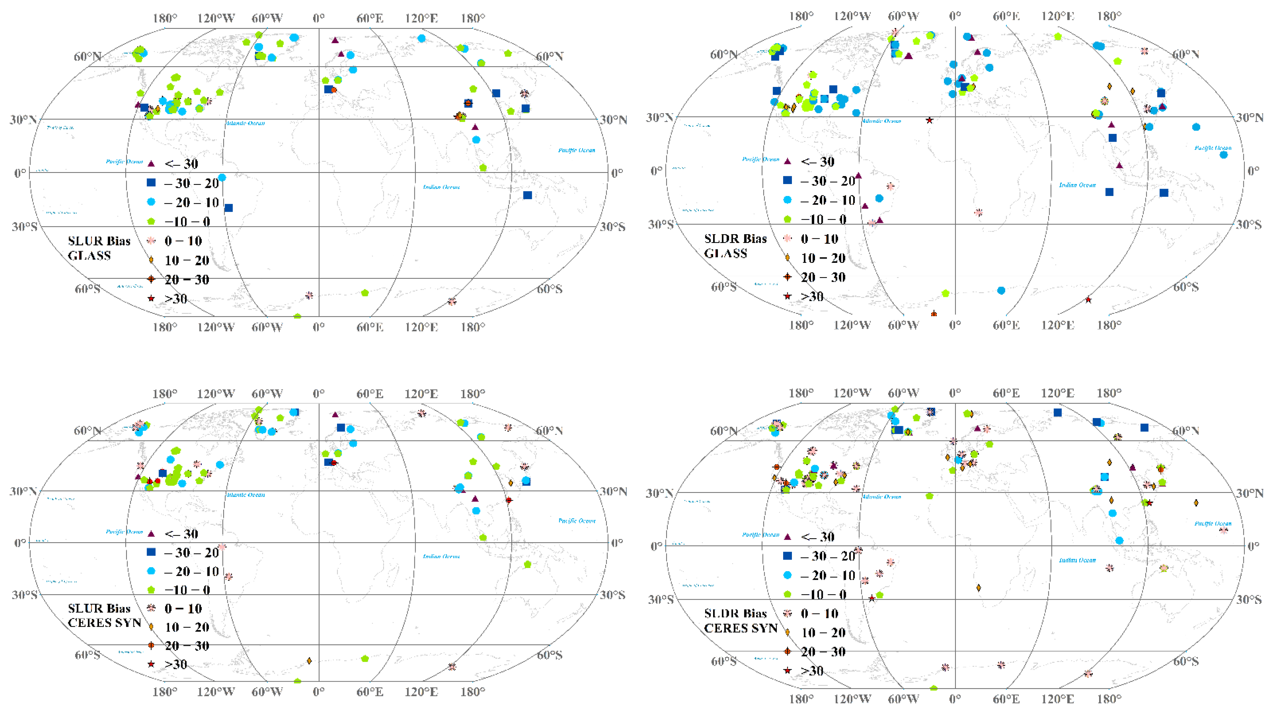
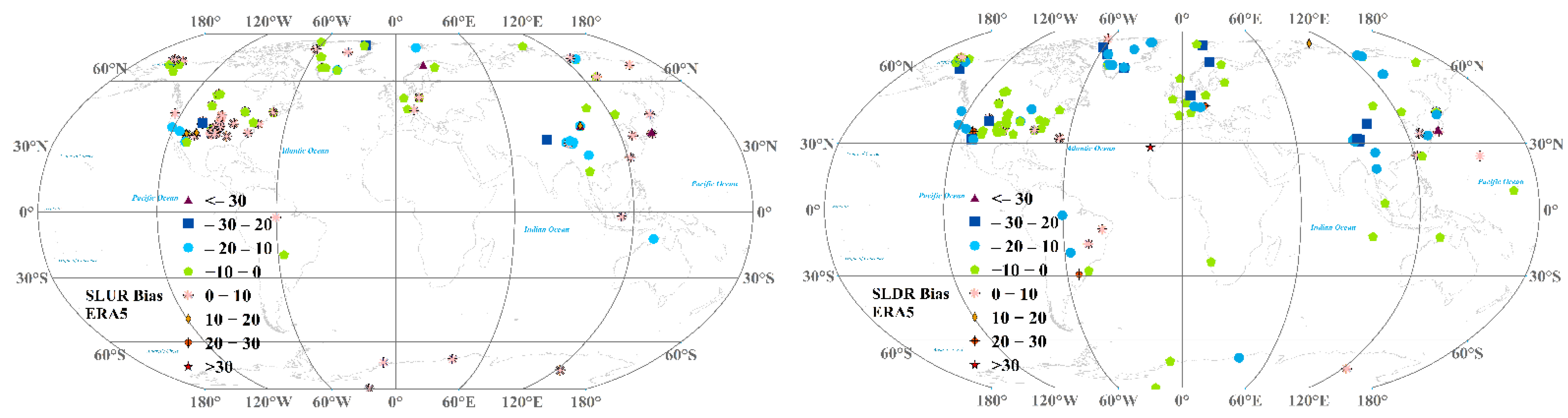
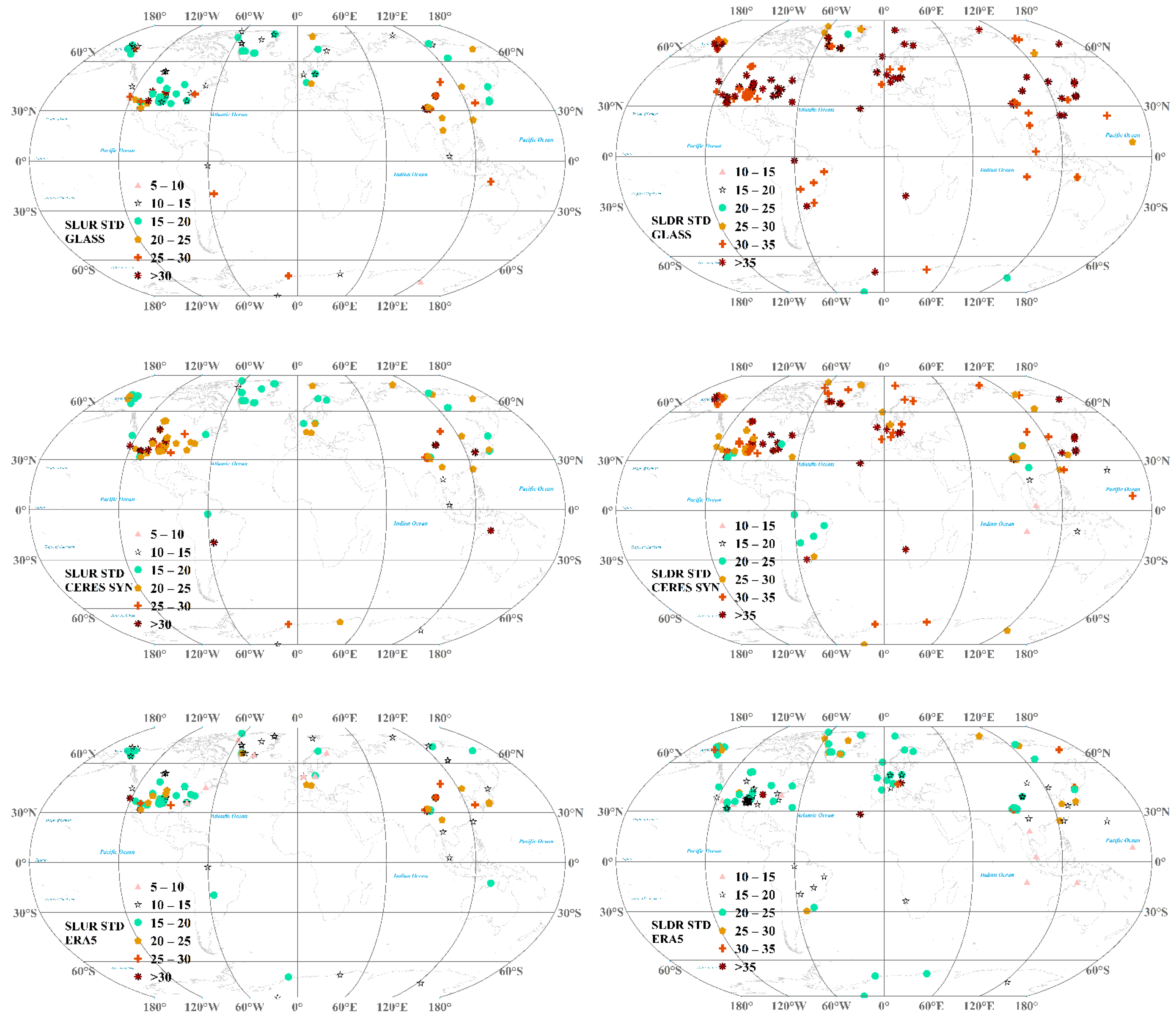
4.1.3. Spatial Distribution of the Validation Results

To further explore the spatial variability of the accuracy of the three surface LW radiation products, the global spatial distributions of the bias, Std and RMSE at each site were determined. The detailed results in North America, Asia, Europe, South America, Antarctica and the Arctic are shown in Appendix Table A1.
Figure 5 shows the spatial distributions of the bias of the SLUR and SLDR for the three surface LW radiation products. As a whole, most sites have negative biases, suggesting that three SLUR products are underestimated. For GLASS and CERES SYN, there are almost always negative biases (−20~0 W/m2). Additionally, there are at least 10 sites located in North America, Asia, the Arctic and Europe with negative biases smaller than −20 W/m2 for GLASS SLUR and positive biases greater than 20 W/m2 for CERES SYN SLUR. For ERA5, positive biases (0~10 W/m2) are mainly widespread in North America, Antarctica and Asia, while negative biases (−10~0 W/m2) are mostly found in North America, the Arctic, Europe and North America, especially the negative biases of six sites that are more than 30 W/m2.
Regarding SLDR, the biases for the three LW radiation products are mainly negative and show a large spatial variation. The biases are −8.22, −9.41 and −5.57 W/m2 for GLASS, ERA5 and CERES SYN SLDR under all-sky conditions, respectively. For GLASS, the negative biases (−30~−10 W/m2) are mainly widespread in North America, Europe, Asia, and the Arctic. The biases in South America are smaller than −30 W/m2, while those in Antarctica are mainly larger than −20 W/m2. For CERES SYN, most sites have positive biases (0~10 W/m2) in the above four subregions. The biases in South America primarily range from −10~10 W/m2, while those in Antarctica are mainly smaller than 10 W/m2. For ERA5, negative biases smaller than −10 W/m2 are prevalent in North America, Europe, Asia and Antarctica. The biases in the Arctic are smaller than −20 W/m2. The biases in South America are mainly in the range of −20~10 W/m2. These results show that the GLASS and ERA5 SLDR tend to be seriously underestimated, which is consistent with the results shown in Table A1.
Figure 6 shows the spatial distribution of the Std of the SLUR and SLDR. The three SLUR products perform better in the Arctic, Antarctica and Europe and worse in Asia. The Stds for the ERA5 SLDR are all smaller than those for GLASS and CERES SYN SLDR. The Stds of GLASS and ERA5 SLUR are lower than those of CERES SYN SLUR. GLASS and ERA5 have a lower Std (10~20 W/m2), mainly in North America, the Arctic, Antarctica, South America and Europe, and are ~10 W/m2 for some sites in North America, the Arctic and Europe, and 20~30 W/m2 in North America and Asia; the corresponding overall Stds are 20.98/19.87, 18.11/16.98, 13.01/12.03, 18.59/14.09, 17.56/15.7 and 26/23.06 W/m2, respectively, as shown in Table A1. The Stds of CERES SYN SLUR mainly range from 15~30 W/m2 in the above regions, and the corresponding overall Stds are mainly more than 23 W/m2, except for Antarctica, which is 16.2 W/m2. The spatial distributions of the Stds for GLASS and CERES SYN have larger spatial heterogeneity than those of ERA5. There are four sites where the Stds for GLASS and CERES SYN exceed 30 W/m2, but only one for ERA5. Overall, the GLASS and ERA5 SLUR products perform better than the CERES SYN product.
Regarding SLDR, ERA5 has the lowest Stds compared to GLASS and CERES SYN. The Stds of ERA5 SLDR range from 10~20 W/m2 in Asia and South America, 15~25 W/m2 in North America, Europe and Antarctica, and 20~30 W/m2 in the Arctic. For CERES SYN, although just a few sites in North America, Asia, and Europe have Stds between 15 and 25 W/m2, the majority of Stds are larger than 30 W/m2 globally. For GLASS, practically all of the Stds are greater than 30 W/m2. As indicated in Table A1, the Stds for GLASS and CERES SYN nearly surpass 30 W/m2 in six subregions, whereas the ERA5 Stds are approximately 25 W/m2. This demonstrates that the spatial distribution of the Stds for the three products is in accordance with the overall Stds in the six subregions shown in Table A1. Taken together, the results indicate that the ERA5 SLDR product performs the best among three SLDR products based on the Std.
Figure 7 shows the spatial distribution of the RMSE of the SLUR and SLDR at each site. The overall trends are similar to those of the Std for SLUR and SLDR. For SLUR, the RMSEs for GLASS and ERA5 are mainly in the range of 10~25 W/m2 and 5~25 W/m2, respectively, while those for CERES SYN are distributed in the range of 15~25 W/m2. The RMSEs for ERA5 in Asia are smaller than those for GLASS and CERES SYN, with values of approximately 30 W/m2. The RMSEs for ERA5 and GLASS are less than 20 W/m2 in Antarctica, but those for CERES SYN are less than 30 W/m2. The corresponding overall RMSEs for ERA5 and GLASS are 21.84/19.87, 20.46/17.23, 13.94/12.53, 23.91/14.1, 20.69/16.48 and 26.5/23.07 W/m2 in North America, the Arctic, Antarctica, South America, Europe and Asia, respectively, whereas those for CERES SYN are approximately 25 W/m2, except that for Antarctica, which is 16.48 W/m2. These results show that the ERA5 and GLASS SLUR products perform better than the CERES SYN SLUR product. The RMSEs for the three SLUR products exhibit a large spatial variability.
As far as SDLR is concerned, the RMSEs for ERA5 are mainly in the range of 15~30 W/m2, and ERA5 performs worse in the Arctic, with all RMSEs greater than 25 W/m2. The RMSEs are mainly greater than 30 W/m2 for GLASS and CERES SYN. Particularly for GLASS, the RMSEs reach 40 W/m2, as shown in Table A1, mainly due to the poor estimation of SLDR under cloudy-sky conditions because the SLDR retrieval is particularly sensitive to errors in certain cloud parameters and atmospheric states [50], especially the cloud phase, cloud base temperature, screen-level temperature and humidity. The SLDR is more susceptible to cloud properties than atmospheric states if cloudiness persists, and satellite-derived SLDR is still inhomogeneous [51], which can also be seen in Figure 6. In addition, the inability of MODIS measurement to see through clouds can also lead to uncertainties in the SLDR [44]. Together, these results demonstrate that the ERA5 SLDR product performs better than the GLASS and CERES SYN SLDR products. A common characteristic of the three SLDR products is that their RMSEs perform poorly in the Arctic.
According to the evaluation results mentioned above, the ERA5 reanalysis product outperforms the GLASS and CERES SYN products. The accuracy of the GLASS SLUR has the best performance under clear-sky conditions. Furthermore, the high spatial resolution GLASS LW radiation product can provide the rich spatial information than cannot be obtained from the coarse resolution ERA5 and CERES SYN surface LW radiation products.

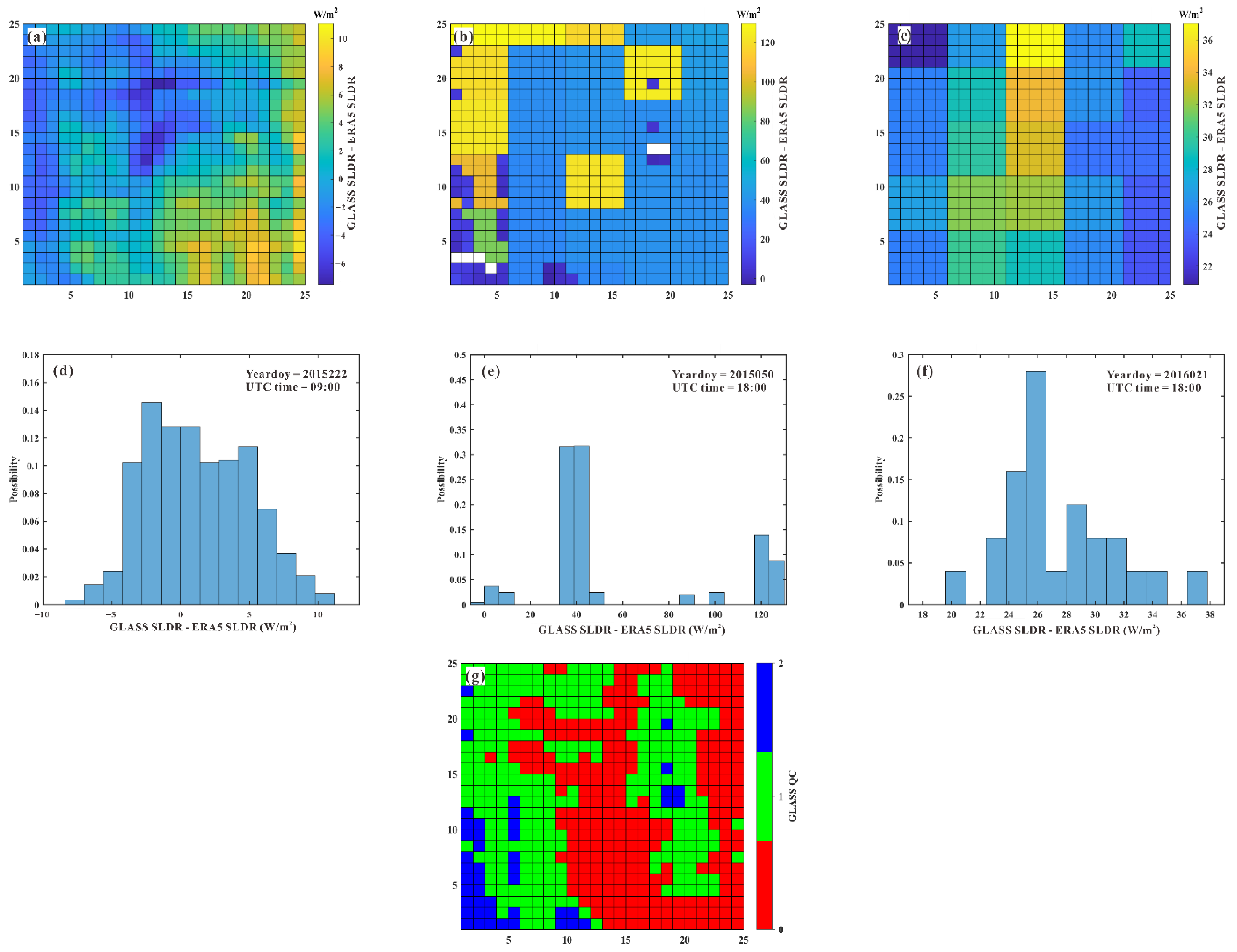
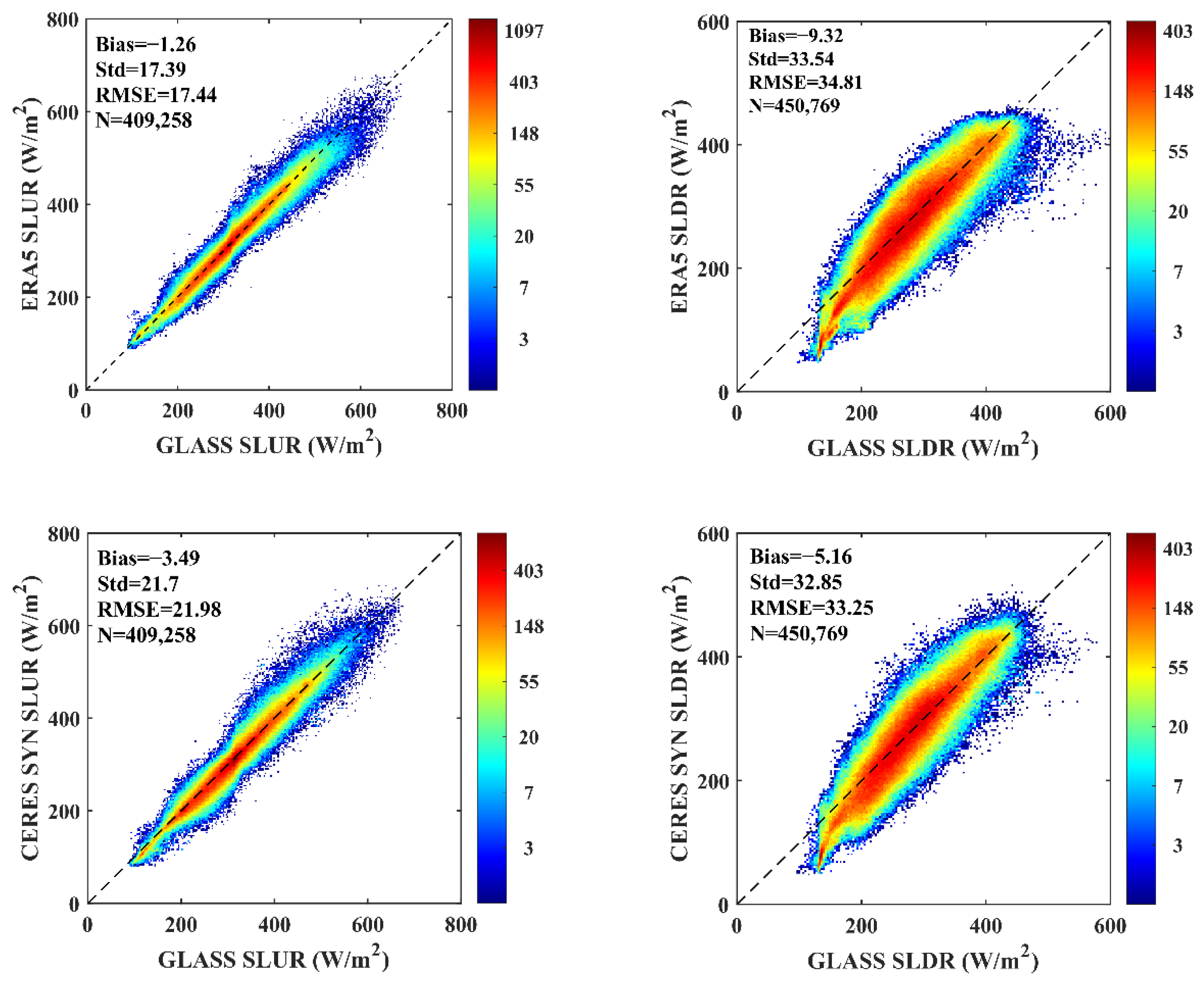
4.2. Cross-Evaluation with the GLASS Surface LW Radiation Product

As shown in Figure 4, SLDR has a strong heterogeneity in 1 km spatial scale, let alone the ERA5 SLDR and CERES SYN SLDR. Usually, flux towers measure SLDR and SLUR with a footprint ranging from tens to hundreds of meters [52]. For example, the BSRN, Ameriflux, Asia, and FLUXNET networks use towers with variable heights that are determined by the height of the trees. The effective heights of most towers are approximately 2~40 m, and the projected FOV on the surface is approximately 18~505 m. As a result, the representativeness of the flux measurements is not sufficient, and the spatial mismatch between the site measurements and satellite pixel or reanalysis grid may cause potential errors in the direct validation, especially for heterogeneous landscapes.
Follow the study of Liang et al. [53], we used the GLASS surface LW radiation product as a bridge to evaluate the CERES SYN and ERA5 surface LW radiation products. The bias of the GLASS surface LW radiation product was first removed using the validation results in Section 4.1.1. For example, if the bias in the GLASS SLUR was positive, we subtracted the positive bias value from the GLASS SLUR and named it the bias-corrected GLASS SLUR, and vice versa. Then, the bias-corrected GLASS surface LW radiation product was aggregated to 0.25° and 1° to evaluate the ERA5 and CERES SYN LW radiation products, respectively. The evaluation results are shown in Figure 8.
The bias, Std and RMSE of ERA5 SLUR are 1.26, 17.39 and 17.44 W/m2, and the values are −3.18, 25.15 and 25.35 W/m2 for CERES SYN SLUR. Compared to the direct valuation results, the bias and Std change very little, whereas the RMSEs decrease by 0.93–3.37 W/m2. The bias, Std and RMSE of ERA5 SLDR are −9.32, 33.54 and 34.81 W/m2, and the values are −5.16, 32.86 and 33.25 W/m2 for CERES SYN SLDR. The absolute values of bias are slightly decreased and the RMSE of ERA5 SLDR increases by 8.79 W/m2, while the RMSE of CERES SYN SLDR decreases by 1.44 W/m2.
As a whole, the evaluation results were not significantly improved using the bias-corrected GLASS surface LW radiation product. We should continue to improve the accuracy of the GLASS surface LW radiation product such as incorporating the topographic effects [54]. In addition, it is also urgent to develop an effective upscaling method suitable for handling large differences in scale.

4.3. Global Annual Mean of Surface LW Radiation

In this section, the global annual mean of surface LW radiation fluxes in the period 2003~2020 were computed using Equation (5) for GLASS, CERES SYN, and ERA5. The M-K test technique was used to compare the spatiotemporal variation in three surface LW radiation products over 18 years.
To characterize the variation in global surface LW radiation, the latitude-weighted average method was used to calculate the global mean surface LW radiation value:
L W ¯ = L W cos ( θ i ) cos ( θ i )
where L W ¯ is the latitude-weighted average, L W i is the grid value of the surface longwave radiation and θ i is the latitude of each grid value. This method does not consider the effect of the area or grid size [55] and can minimize the effect of differences in the actual area among product grids at different latitudes [56].

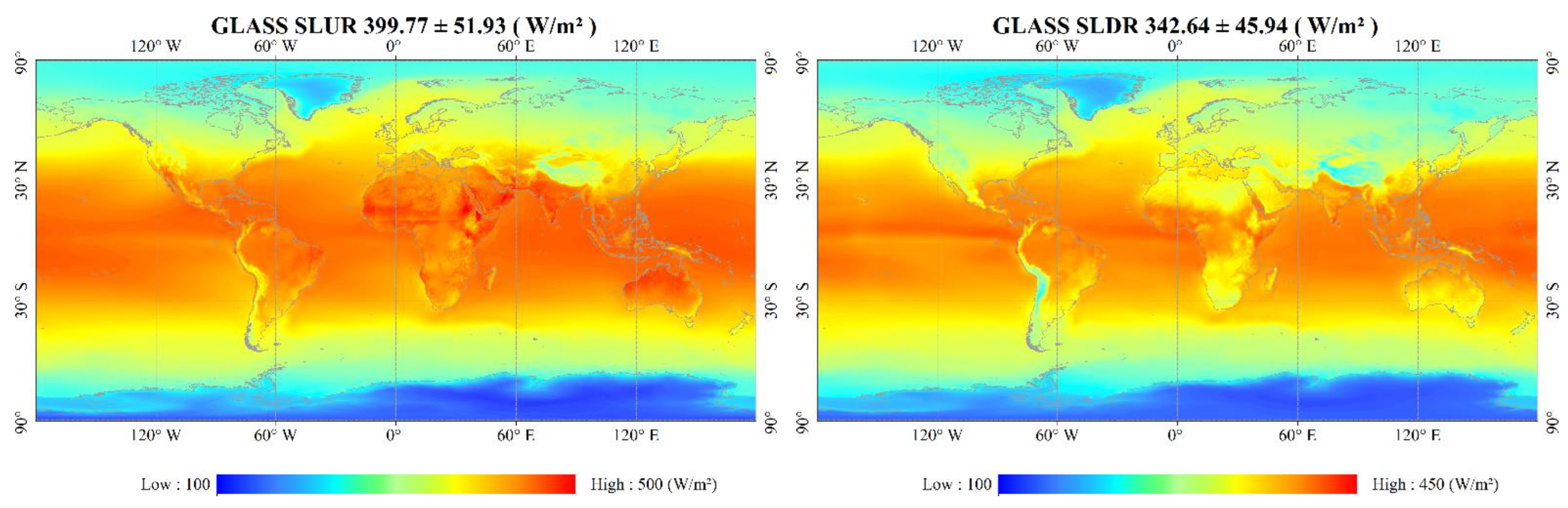
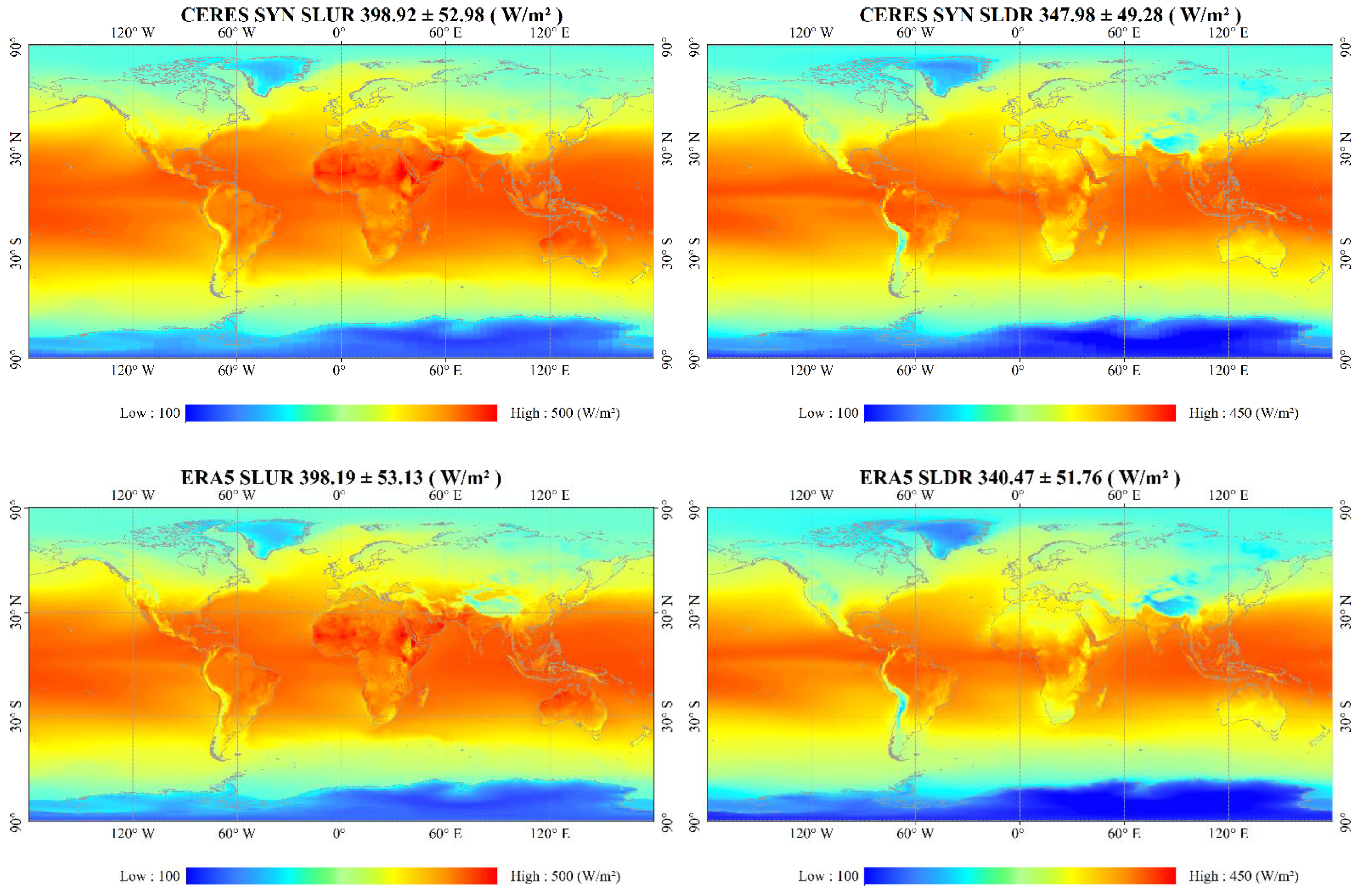
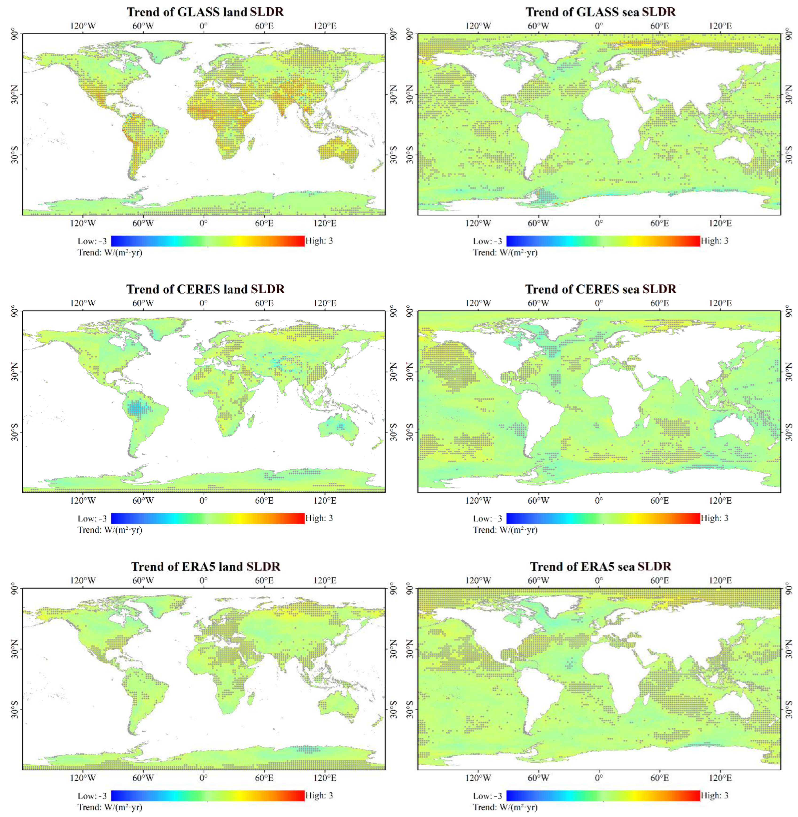
4.3.1. Spatial Distribution of the Global Annual Mean Surface LW Radiation

Figure 9 shows the geographical distribution of the global annual mean SLUR and SLDR over the period 2003~2020. The spatial patterns are consistent and agree in magnitude. The surface LW radiation values steadily decrease from the middle and low latitudes toward the north and south poles. The annual mean SLUR and SLDR at the North Pole are usually greater than those in Antarctica, which indicates that Antarctica is colder than the Arctic, as reflected in the differences in surface temperature. Greenland is also colder than the other Arctic regions. At the boundary of Antarctica, the annual mean SLUR and SLDR begin to increase slowly along the ocean and are consistent with those of the North Pole. Note that the SLUR and SLDR values of the Qinghai–Tibet Plateau (TP) are relatively lower than those of its surrounding regions due to its complex climatic conditions and terrain, even though the TP is located in the middle latitudes. It is worth noting that the annual mean values of ERA5 SLDR distributed in the western TP are lower than those of the GLASS and CERES SLDR. In addition, the SLUR is larger in the Sahara, Kalahari, Australian and Arabian Deserts at mid- and low latitudes (15~35°N and 15~35°S), while it is relatively lower in the Taklimakan and Turkestan Deserts. However, for the above deserts, the SLDR is larger near the equator. The desert in the former is warmer because of the climate, and that in the latter is colder because of the terrain. The same cause is at work in the Andes mountains, where the SLUR and SLDR are evidently lower than those in the surrounding geographical areas.
The global mean statistics of the surface LW radiation are listed in Table 3. The global mean GLASS, CERES SYN and ERA5 SLUR are 399.77, 398.92 and 398.19 W/m2, respectively. The values are close to those reported by previous studies [22,26,28,29]. The differences among these global mean SLURs are less than 1~2 W/m2 worldwide.
The land mean SLUR for GLASS, CERES SYN and ERA5 are 378.98, 380 and 375.20 W/m2, within a range of 5 W/m2 or less. The land mean SLUR here is approximately 3~9 W/m2 larger than that of ERA-Interim (370.6), ERA-40 (371.0), JRA-25 (372) and NRA2 (369.1) calculated by Berrisford, Kållberg, Kobayashi, Dee, Uppala, Simmons, Poli and Sato [26]. The ocean mean SLUR for GLASS, CERES SYN and ERA5 are 408, 409.26 and 408.38 W/m2, respectively, which are consistent within 1.5 W/m2. The ocean mean SLUR for four different reanalysis products are 408.6, 408.5, 409.7 and 407.9 W/m2 by Berrisford, Kållberg, Kobayashi, Dee, Uppala, Simmons, Poli and Sato [26]; the ocean mean SLUR for CMIP5 climate models (2000–2005) is 409 W/m2 by Wild, Folini, Hakuba, Schär, Seneviratne, Kato, Rutan, Ammann, Wood and König-Langlo [25]. Here, the ocean mean SLUR for GLASS, CERES SYN and ERA5 over the period 2003–2020 match well with those in previous studies, which indicates that the ocean SLUR remains unchanged from then to now, whereas the land mean SLUR shows a slight increasing tendency.
There are large differences in the calculation of the global mean SLDR by different researchers. The global mean GLASS, CERES SYN and ERA5 SLUR SLDR are 342.64, 347.98 and 340.47 W/m2, respectively. The difference is as high as 7.51 W/m2. The global mean SLDR difference is 12.6 W/m2 from the previous studies in Table 3. If we did not consider the value from Trenberth et al. [2] that calculates the global mean values with two years’ data, the difference is within 4.6 W/m2. The changing trend of the global mean SLDR from CERES is reasonable, i.e., increasing from 333 W/m2 to 347.97 W/m2, in the context of global warming.
The land mean SLDR of GLASS, CERES SYN and ERA5 are 311.34, 322.38 and 308.39 W/m2, the corresponding values are 355.86, 361.96 and 354.95 W/m2 over ocean, respectively. The differences are relatively larger than those at the global level. The SLDRs of GLASS and ERA5 are close to the estimate of 307 ± 3 W/m2 over land and 356 ± 3 W/m2 over the ocean in Wang and Dickinson [57].
Table 3. Comparison of the global mean surface LW radiation calculated from different data sources.
ProductsSLUR (W/m2)SLDR (W/m2)TimeReference
CERES early396333March 2002–May 2004Trenberth, Fasullo and Kiehl [2]
ERA-Interim397.7341.21989–2008Berrisford, Kållberg, Kobayashi, Dee, Uppala, Simmons, Poli and Sato [26]
CERES398345.62000–2010Stephens, Li, Wild, Clayson, Loeb, Kato, L’Ecuyer, Stackhouse, Lebsock and Andrews [22]
CERES EBAF398344March 2000–February 2010Kato, et al. [58]
CERES, ISCCP-FD, 2B-FLXHR-lidar and C3M3993412000–2009L’Ecuyer, Beaudoing, Rodell, Olson, Lin, Kato, Clayson, Wood, Sheffield and Adler [28]
43 CMIP5 climate models, ERA399.9343.82000–2014Wild [29]
GLASS399.77/378.98/408.54342.64/311.34/355.862003–2020This study
CERES SYN398.92/380/409.26347.98/322.38/361.962003–2020This study
ERA5398.19/375.38/408.38340.47/308.39/354.952003–2020This study
Note: The global mean SLUR and SLDR for GLASS, CERES SYN and ERA5 represent the globe, land and ocean from left to right.
In short, the global annual means of the GLASS, CERES SYN and ERA5 SLUR are less than 400 W/m2, and those of the SLDR are slightly above 340 W/m2, which is consistent with recent findings.

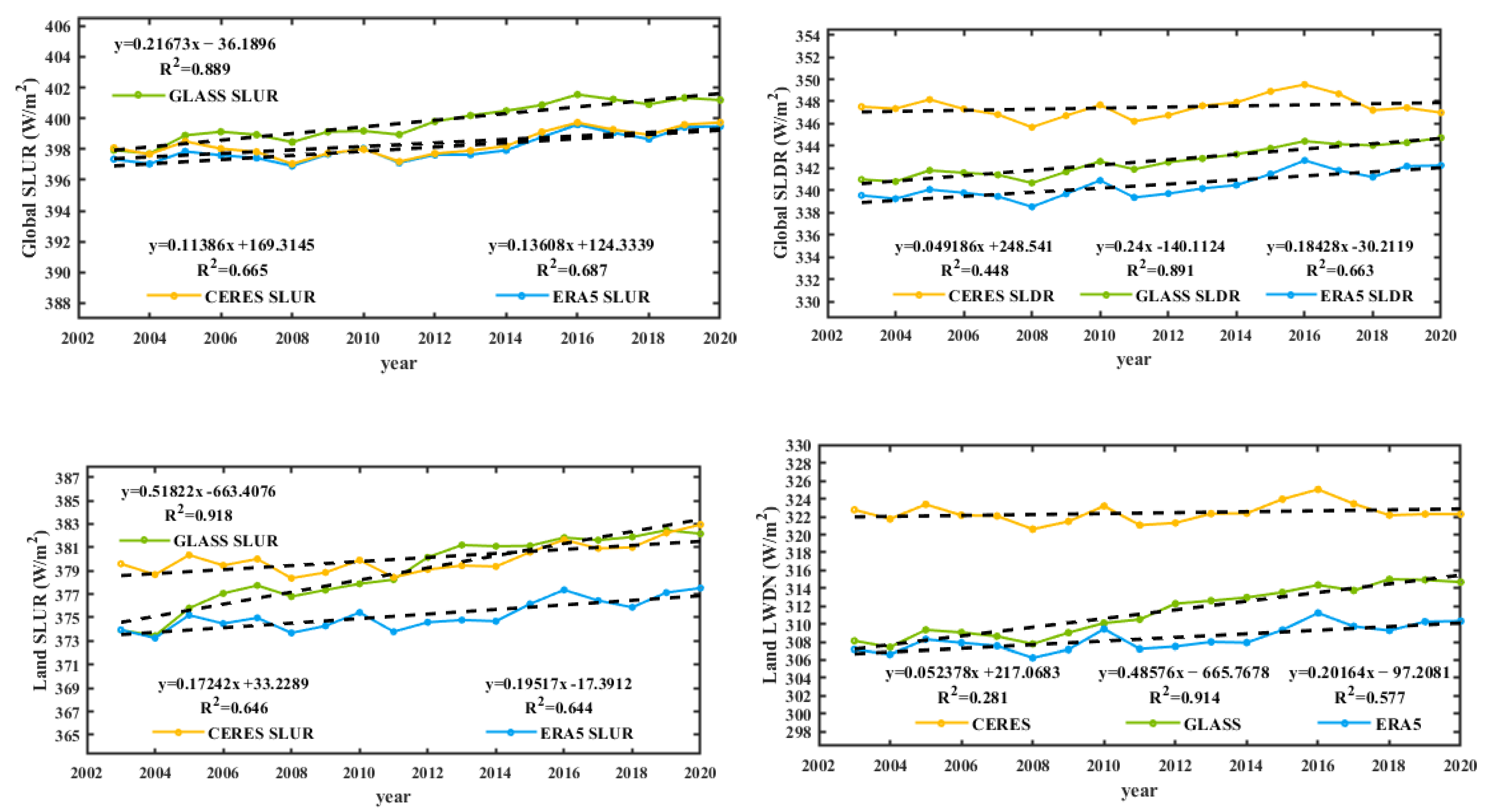
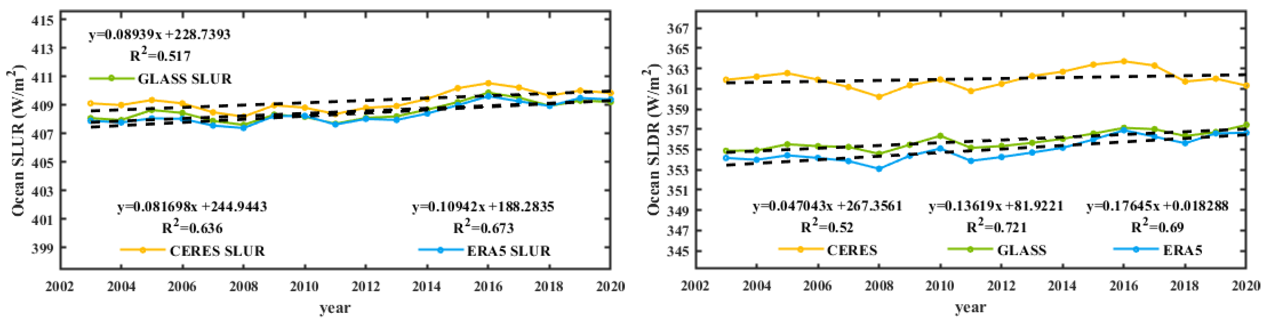
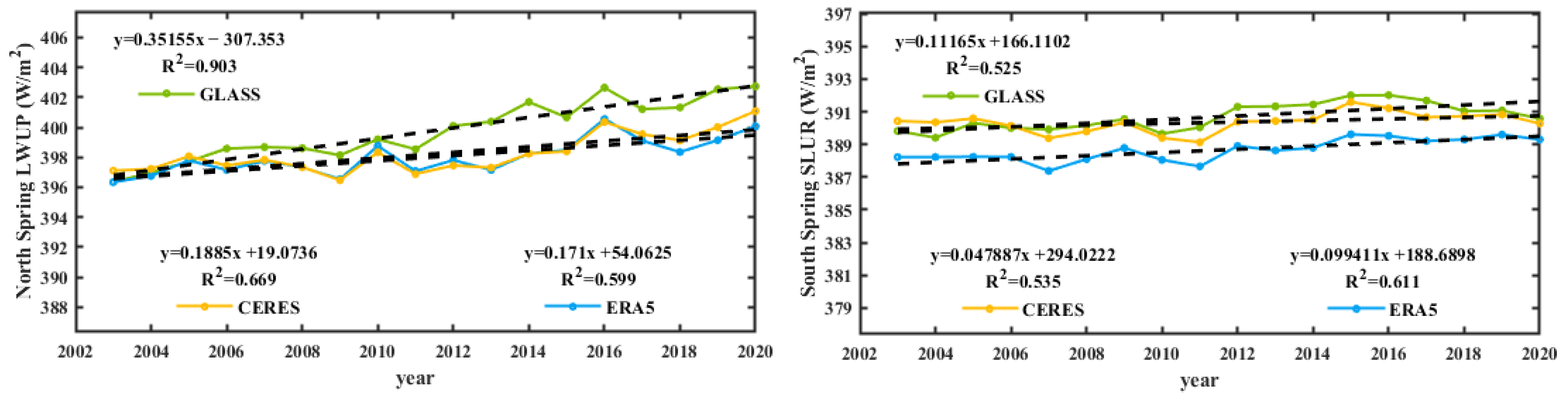
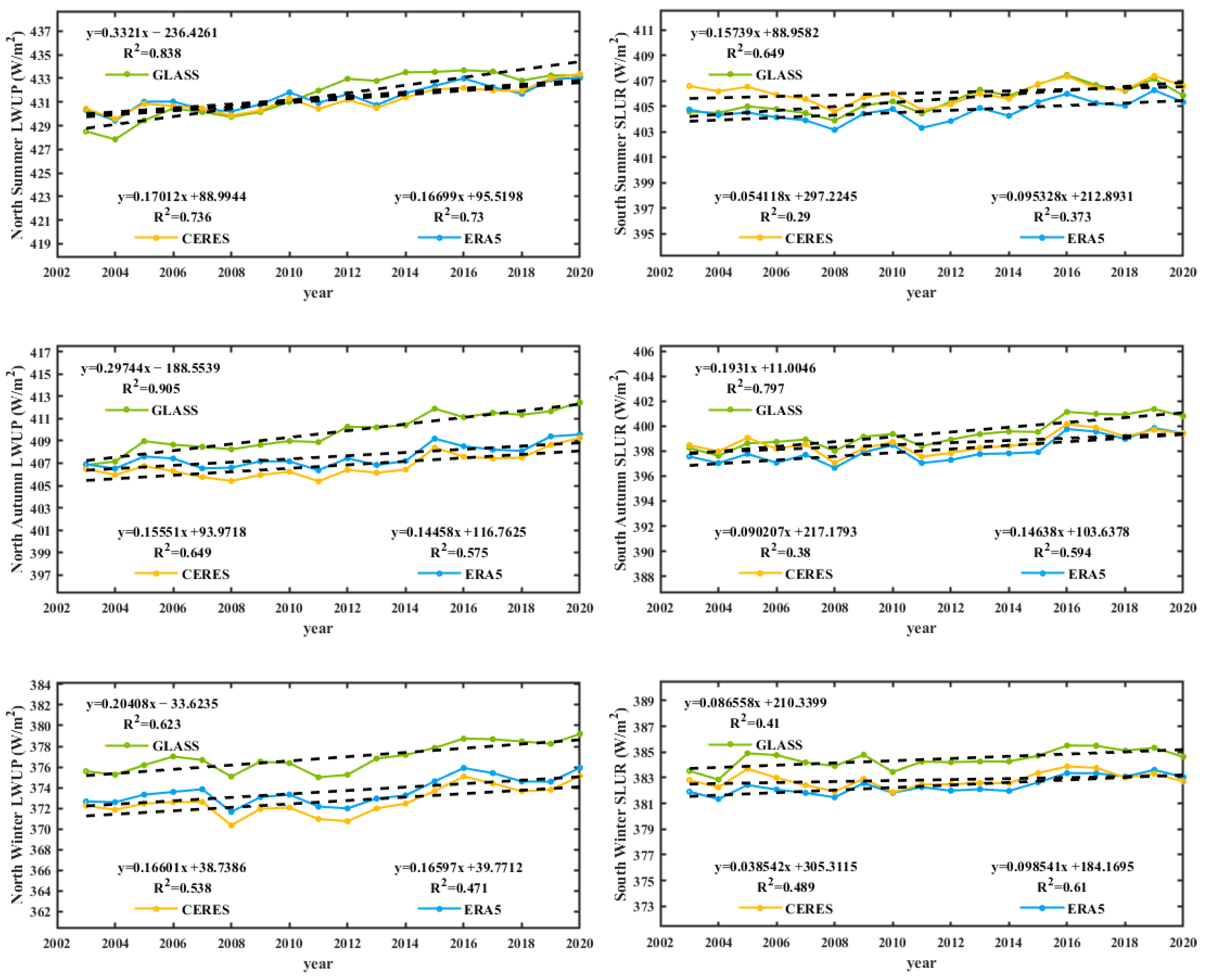
4.3.2. Temporal Variation in the Annual Mean Surface LW Radiation

We calculated the temporal change trend (i.e., annual change rate) of the surface SLDR at each grid by the M-K test method, and the results for SLDR are shown in Figure 10. On land, the annual change rate of the GLASS SLDR clearly increased in some regions located in low- and mid-latitude land areas. There is a growth of 2~3 W/m2 per year in Africa, South and East Asia, and North and South America, and about 1 W/m2 per year in Eastern Europe and North Asia. Almost 90% of significant trends are positive trends in Australia and South America. The annual change rate of the CERES SYN SLDR slightly increased in Eastern Europe and North Asia, similar to that of GLASS SLDR. There is apparently a decline of 1~2 W/m2 per year in South America and Australia, contrary to that of the GLASS SLDR. The annual change rate of the ERA5 SLDR also slightly increased in Eastern Europe and North Asia, similar to that of the GLASS and CERES SYN SLDR. In other regions, there is a slightly increased and sporadic distribution. The ERA5 SLDR shows no obvious annual change rate compared to the GLASS and CERES SYN SLDR.
For the ocean, the annual change rate of the GLASS SLDR clearly increased in the Arctic Ocean, especially in the areas above Eastern Europe and North Asia, with growth of 1~2 W/m2 per year. There is an increase of 0.5~1 W/m2 per year in the North Pacific, North Atlantic, Indian and North Atlantic Ocean, and a clear decrease amount of about 1 W/m2 per year in the Weddell Sea. The annual change rate of CERES SYN SLDR has a growth of about 1 W/m2 per year in the Arctic Ocean above Eastern Europe and North Asia, the North Pacific and South Pacific Ocean close to North and South America, and the Indian Ocean, while there is a decline of 1 W/m2 per year in the North Atlantic Ocean close to Greenland and the Pacific Ocean near the Australia coast. The annual change rate of ERA5 SLDR slightly increased by 1 W/m2 per year in the Arctic Ocean, North Pacific Ocean, North Atlantic, and South Pacific Ocean close to the Australia coast.
Generally, the GLASS SLDR shows clear increasing trends in the majority of areas where the global warming effect is exacerbated year after year. The CERES SYN SLDR indicates a decrease in Australia and South America. By contrast, the annual change rate of ERA5 SLDR has no obvious decrease or increase. There may be two reasons for this: (1) the M-K test is more accurate at fine spatial scales and can better describe surface types or variables with trends over time [59], and (2) there are significant uncertainties in the surface LW radiation information offered by different datasets, as demonstrated in Section 4.1, which have not been addressed [22]. The spatial distributions of SLUR variation rates for the three products are similar to those of SLDR variation rates, and are not analyzed in this paper.
Figure 11 displays the temporal variations in the global annual mean surface LW radiation. For the annual mean SLUR, the linear trends for CERES SYN are similar to those of ERA5 for the globe and land, 0.11/0.13 W/m2 globally and 0.17/0.19 W/m2 on land, respectively. GLASS shows an obvious increasing trend globally and on land, particularly on land, with a trend of 0.51 W/m2 per year. For the ocean, the temporal fluctuations and values of the three SLUR products, particularly GLASS, practically overlap.
For the annual mean SLDR, the linear trends are 0.05/0.18/0.24 W/m2 globally, 0.05/0.20/0.48 W/m2 on land and 0.05/0.18/0.14 W/m2 in the ocean for the CERES SYN, ERA5 and GLASS SLDR, respectively. GLASS has an apparent growing tendency both globally and on land compared with ERA5; GLASS shows a trend of 0.49 W/m2 per year on the land, and the difference in the annual mean of both increases with time. For the ocean, the linear trends in GLASS and ERA5 are consistent, and the curves nearly overlap. The CERES SYN has almost no linear trend over the globe, land and ocean.
The seasonal properties of the SRB also fundamentally influence the regional climate and its variability. Figure 12 depicts the seasonal fluctuations in the annual mean SLUR in the Southern Hemisphere (SH) and Northern Hemisphere (NH). In contrast to those in the SH, the annual mean SLUR during four seasons in the NH displays rising linear trends. From spring to winter in the NH, the linear trends of GLASS vary from 0.35 to 0.2 W/m2 per year, while those of CERES SYN are 0.19, 0.17, 0.16 and 0.17 W/m2 by season and those of ERA5 are 0.17, 0.16, 0.14 and 0.17 W/m2, which indicates that the linear trends in CERES SYN are comparable to those in ERA5 throughout the four seasons in the NH. In the SH, the linear trends of GLASS are 0.19, 0.09, 0.11 and 0.16 W/m2 and those of the ERA5 are 0.15, 0.1, 0.1, and 0.1 W/m2 in autumn, winter, spring and summer, respectively. The linear trends of GLASS are larger than those for ERA5 in the SH. CERES SYN has no obvious linear trends and are less than 0.09 W/m2. Compared with the NH, the linear trends for the three products in the SH are relatively lower. The above results show that the SLUR is very asymmetrical during the four seasons in the Northern and Southern Hemispheres.
Figure 13 shows the seasonal variations in the annual mean SLDR of the Southern and Northern Hemispheres. The annual mean SLDR of CERES SYN throughout the four seasons remains almost unchanged in the NH and SH. From spring to winter in the NH, the varying linear trends of GLASS from 0.35, 0.35, 0.33 and 0.23 show growing tendencies compared with those of ERA5, which are 0.21, 0.23, 0.23 and 0.21 W/m2 by season. Only in winter does the linear trend of GLASS coincide with that of ERA5. A similar situation also occurs during the four seasons in the SH, but the linear trends in GLASS and ERA5 are slightly weaker than those in the NH. This demonstrates that the linear trends in SLDR are also very asymmetrical during the four seasons in the Northern and Southern Hemispheres.
In summary, the three LW radiation products produce substantially different long-term trends in the annual mean SLUR and SDLR. The linear trends in the global and land mean CERES SYN SLUR are similar to those of ERA5. The linear trends of the ocean mean that GLASS SLUR and SLDR are in agreement with those of ERA5. The long-term trends of the seasonal mean SLUR and SDLR in the NH and SH are asymmetrical. This is a result of the asymmetrical atmospheric heat transport across the equator [60]. Evidently, the seasonal increase tendency of the SLUR and SDLR in the NH is greater than that in the SH.

5. Conclusions

Accurate estimates of surface LW radiation and its temporal changes are important for determining global energy and hydrological cycles and understanding climate sensitivity. This study quantifies (1) the accuracies of surface LW radiation from GLASS, CERES SYN and ERA5 products with 181 sites collected from 10 different flux networks and (2) global annual mean values and its temporal variation from 2003–2020.
According to the direct validation, the global accuracies of the ERA5 SLUR and SLDR are the best, with bias/Std/RMSE values of −1.05/18.34/18.37 W/m2 for SLUR and −9.41/24.15/25.92 W/m2 for SLDR, respectively. The performance of the GLASS SLUR is better than that of the ERA5 SLUR under clear-sky conditions, with a bias/Std/RMSE of −6.75/14.18/15.17 W/m2. The CERES SYN SLUR has a bias/Std/RMSE of −3.18/25.15/25.35 W/m2. The accuracy of two satellite SLDRs (GLASS and CERES SYN SLDR) is comparable, but poorer than that of the ERA5 SLDR, with bias/Std/RMSE values of −8.22/36.71/37.62 W/m2 and −5.57/34.22/34.67 W/m2, respectively. The bias/Std/RMSE of ERA SLDR are −9.41/24.14/25.92 W/m2. Compared to coarse resolution surface LW radiation product, GLASS LW radiation can provide rich spatial details due to its high spatial resolution. In addition, we are updating the production of the cloudy-sky SLUR using our newly developed cloudy-sky land surface temperature retrieval algorithms and products [61,62,63,64,65,66], and updating the cloudy-sky SLDR production using the cloud base temperature [48,67]. The accuracy of the GLASS cloudy-sky SLUR and SLDR could be improved.
When the bias-corrected GLASS surface LW radiation products were used to evaluate the coarse resolution CERES SYN and ERA5 surface LW radiation products, the evaluation results were not significantly improved compared to the direct validation. Both the algorithms for producing the GLASS surface LW radiation product and the upscaling method for generate coarse resolution surface LW radiation product should be improved in the future.
The spatial distributions of the global annual mean for the GLASS, CERES SYN and ERA5 SLUR and SLDR are consistent in spatial pattern and agree in magnitude. The global annual mean SLUR for GLASS, CERES SYN and ERA5 are 399.77, 398.92 and 398.19 W/m2, and SLDR are 342.64, 347.98 and 340.47 W/m2, respectively, which are in line with the previous findings.
Varying degrees of long-term increasing trends appeared in the global mean SLUR and SDLR of the three LW radiation products. The linear trends in the global and land mean GLASS SLUR and SLDR show obvious growing tendencies, followed by ERA5 and CERES SYN. The long-term trends of the seasonal mean SLUR and SDLR in the Northern and Southern Hemispheres are very asymmetrical. The seasonal increasing tendency of the SLUR and SDLR in the Northern Hemisphere is greater than that in the Southern Hemisphere.

Author Contributions

Conceptualization, J.C.; methodology, Q.Z.; validation, Q.Z.; formal analysis, Q.Z.; investigation, Q.Z.; resources, J.C.; data curation, Q.Z. and M.G; writing—original draft preparation, Q.Z.; writing—review and editing, J.C.; visualization, Q.Z. and M.G.; supervision, J.C.; project administration, J.C.; funding acquisition, J.C. All authors have read and agreed to the published version of the manuscript.

Funding

This research was funded by the National Natural Science Foundation of China under Grants 42192581 and 42071308.

Data Availability Statement

The GLASS products can be downloaded from http://www.glass.umd.edu, accessed on 5 June 2023 or http://www.geodata.cn/thematicView/GLASS.html, accessed on 5 June 2023. The ERA5 reanalysis datasets can be downloaded from https://cds.climate.copernicus.eu/cdsapp#!/dataset/reanalysis-era5-singlelevels?tab=form, accessed on 5 June 2023. The CERES_SYN products used in this work were downloaded from https://ceres-tool.larc.nasa.gov/ord-tool/jsp/SYN1degEd41Selection.jsp, accessed on 5 June 2023. We are very grateful to these organizations for providing the data we used in this study.

Conflicts of Interest

The authors declare no conflict of interest.

Appendix A

Table A1. Accuracies of the GLASS, ERA5 and CERES SYN SLUR and SLDR in regional and continental scales.
RegionProductSky ConditionsSLUR (W/m2)SLDR (W/m2)
BiasStd_BiasRMSEBiasStd_BiasRMSE
North AmericaGLASSAll-sky−6.0720.9821.84−7.0436.1936.87
Clear-sky−5.0614.6115.46−5.2124.6325.17
Cloud-sky−4.8221.5122.05−14.3638.1840.79
ERA5All-sky0.219.8719.87−621.6222.44
Clear-sky−3.4421.8222.09−4.0818.819.24
Cloud-sky1.3819.0419.09−6.6122.4223.38
CERES SYNAll-sky1.8829.1729.232.134.9535.01
Clear-sky−1.4626.4726.519.3633.7235
Cloud-sky2.9729.9230.07−0.2335.0235.02
AsiaGLASSAll-sky−5.132626.5−11.739.5941.29
Clear-sky−7.8919.721.22−8.2624.8626.19
Cloud-sky−3.3626.4326.64−16.6841.0744.33
ERA5All-sky−0.5223.0623.07−13.9224.928.53
Clear-sky−4.0424.9925.32−13.7121.5625.55
Cloud-sky−0.1122.7922.79−13.9425.2328.82
CERES SYNAll-sky−0.6327.2427.24−7.233.0333.81
Clear-sky−6.3722.923.774.5434.2634.56
Cloud-sky0.0527.6327.63−8.4432.6633.73
EuropeGLASSAll-sky−10.9317.5620.69−15.7735.5438.88
Clear-sky−9.4313.116.15−4.9419.3619.98
Cloud-sky−9.6316.1218.78−22.7634.5341.36
ERA5All-sky−5.0115.716.48−9.0621.0322.9
Clear-sky−5.6419.4820.28−4.6513.1713.96
Cloud-sky−4.9615.3516.13−9.3921.4723.43
CERES SYNAll-sky−7.3621.5622.78−5.6632.9633.44
Clear-sky−3.1923.824.013.3431.2231.39
Cloud-sky−7.6921.3422.68−6.3332.9833.59
South AmericaGLASSAll-sky−15.0518.5923.91−7.7435.6736.5
Clear-sky−11.88.9214.791.8622.9723.05
Cloud-sky−12.4117.6721.59−15.6435.3638.66
ERA5All-sky0.3314.0914.1−4.4325.0325.42
Clear-sky−8.3712.515.043.5623.4523.72
Cloud-sky0.4314.0814.09−5.0625.0525.55
CERES SYNAll-sky3.8523.8824.191.6831.3731.42
Clear-sky−3.7620.4520.7916.193034.09
Cloud-sky3.9323.924.230.5531.231.2
AntarcticaGLASSAll-sky−513.0113.9412.235.2237.27
Clear-sky−1.748.718.8837.416.5940.91
Cloud-sky−7.114.616.23−8.7131.7532.93
ERA5All-sky3.4912.0312.53−8.6424.8326.29
Clear-sky−1.5813.1313.22−13.9321.5925.69
Cloud-sky4.3111.6412.41−7.7825.2126.39
CERES SYNAll-sky−3.0516.216.48−4.5631.631.93
Clear-sky0.0212.3912.395.9627.6628.29
Cloud-sky−3.5416.6817.05−6.2631.8732.48
ArcticGLASSAll-sky−9.5218.1120.46−13.234.6937.12
Clear-sky−10.6713.6917.35−3.292626.2
Cloud-sky−8.3817.7819.66−16.6734.9838.75
ERA5All-sky−2.9316.9817.23−12.2525.9128.66
Clear-sky−6.218.2519.28−19.1323.6730.44
Cloud-sky−2.5916.8117.01−11.5426.0228.47
CERES SYNAll-sky−7.0722.423.49−12.0134.2136.26
Clear-sky−5.9218.0619.01−4.0132.5832.82
Cloud-sky−7.1922.823.91−12.8434.2736.6
GlobeGLASSAll-sky−7.6319.520.94−8.2236.7137.62
Clear-sky−6.7514.1815.72.6128.0228.14
Cloud-sky−7.0115.9620.78−15.8636.1839.5
ERA5All-sky−1.0518.3418.37−9.4124.1425.92
Clear-sky−4.1720.5220.94−9.1621.3923.26
Cloud-sky−0.4817.8517.86−9.4524.5926.35
CERES SYNAll-sky−3.1825.1525.35−5.5734.2234.67
Clear-sky−2.8523.2823.465.2933.0733.49
Cloud-sky−3.2425.4725.68−7.4234.0634.86

References

  1. Stephens, G.L.; L’Ecuyer, T. The Earth’s energy balance. Atmos. Res. 2015, 166, 195–203. [Google Scholar] [CrossRef]
  2. Trenberth, K.E.; Fasullo, J.T.; Kiehl, J. Earth’s Global Energy Budget. Bull. Amer. Meteorol. Soc. 2009, 90, 311–323. [Google Scholar] [CrossRef] [Green Version]
  3. Liang, S.; Wang, D.; He, T.; Yu, Y. Remote sensing of Earth’s energy budget: Synthesis and review. Int. J. Digit. Earth 2019, 12, 737–780. [Google Scholar] [CrossRef] [Green Version]
  4. Zhang, Y.C.; Rossow, W.; Lacis, A. Calculation of surface and top of atmosphere radiative fluxes from physical quantities based on ISCCP data sets: 1. Method and sensitivity to input data uncertainties. J. Geophys. Res. Atmos. 1995, 100, 1149–1165. [Google Scholar] [CrossRef]
  5. Zhang, Y.C.; Rossow, W.B.; Lacis, A.A.; Oinas, V.; Mishchenko, M.I. Calculation of radiative fluxes from the surface to top of atmosphere based on ISCCP and other global data sets: Refinements of the radiative transfer model and the input data. J. Geophys. Res. Atmos. 2004, 109, 1–27. [Google Scholar] [CrossRef] [Green Version]
  6. Fu, Q.; Liou, K.N. Parameterization of the radiative properties of cirrus clouds. J. Atmos. Sci. 1993, 50, 2008–2025. [Google Scholar] [CrossRef]
  7. Pinker, R.T.; Tarpley, J.D.; Laszlo, I.; Mitchell, K.E.; Houser, P.R.; Wood, E.F.; Schaake, J.C.; Robock, A.; Lohmann, D.; Cosgrove, B.A.; et al. Surface radiation budgets in support of the GEWEX Continental-Scale International Project (GCIP) and the GEWEX Americas Prediction Project (GAPP), including the North American Land Data Assimilation System (NLDAS) Project. J. Geophys. Res. Atmos. 2003, 108, 1–18. [Google Scholar] [CrossRef]
  8. Doelling, D.R.; Loeb, N.G.; Keyes, D.F.; Nordeen, M.L.; Morstad, D.; Nguyen, C.; Wielicki, B.A.; Young, D.F.; Sun, M. Geostationary enhanced temporal interpolation for CERES flux products. J. Atmos. Ocean. Technol. 2013, 30, 1072–1090. [Google Scholar] [CrossRef]
  9. Doelling, D.R.; Sun, M.; Nguyen, L.T.; Nordeen, M.L.; Haney, C.O.; Keyes, D.F.; Mlynczak, P.E. Advances in geostationary-derived longwave fluxes for the CERES synoptic (SYN1deg) product. J. Atmos. Ocean. Technol. 2016, 33, 503–521. [Google Scholar] [CrossRef]
  10. Hersbach, H.; Bell, B.; Berrisford, P.; Hirahara, S.; Horányi, A.; Muñoz-Sabater, J.; Nicolas, J.; Peubey, C.; Radu, R.; Schepers, D.; et al. The ERA5 global reanalysis. Q. J. R. Meteorolog. Soc. 2020, 146, 1999–2049. [Google Scholar] [CrossRef]
  11. Stackhouse, P.W., Jr.; Gupta, S.K.; Cox, S.J.; Zhang, T.; Mikovitz, J.C.; Hinkelman, L.M. The NASA/GEWEX surface radiation budget release 3.0: 24.5-year dataset. Gewex News 2011, 21, 10–12. [Google Scholar]
  12. Draper, C.S.; Reichle, R.H.; Koster, R.D. Assessment of MERRA-2 land surface energy flux estimates. J. Clim. 2018, 31, 671–691. [Google Scholar] [CrossRef]
  13. Von Schuckmann, K.; Palmer, M.; Trenberth, K.E.; Cazenave, A.; Chambers, D.; Champollion, N.; Hansen, J.; Josey, S.; Loeb, N.; Mathieu, P.-P. An imperative to monitor Earth’s energy imbalance. Nat. Clim. Chang. 2016, 6, 138–144. [Google Scholar] [CrossRef] [Green Version]
  14. Liang, S.; Cheng, J.; Jia, K.; Jiang, B.; Liu, Q.; Xiao, Z.; Yao, Y.; Yuan, W.; Zhang, X.; Zhao, X. The global Land surface satellite (GLASS) product suite. Bull. Amer. Meteorol. Soc. 2021, 102, E323–E337. [Google Scholar] [CrossRef]
  15. Gui, S.; Liang, S.; Li, L. Evaluation of satellite-estimated surface longwave radiation using ground-based observations. J. Geophys. Res. 2010, 115, 1–16. [Google Scholar] [CrossRef] [Green Version]
  16. Kratz, D.P.; Gupta, S.K.; Wilber, A.C.; Sothcott, V.E. Validation of the CERES Edition-4A Surface-Only Flux Algorithms. J. Appl. Meteorol. Climatol. 2020, 59, 281–295. [Google Scholar] [CrossRef]
  17. Tang, W.; Qin, J.; Yang, K.; Zhu, F.; Zhou, X. Does ERA5 outperform satellite products in estimating atmospheric downward longwave radiation at the surface? Atmos. Res. 2021, 252, 105453. [Google Scholar] [CrossRef]
  18. Wang, G.; Wang, T.; Xue, H. Validation and comparison of surface shortwave and longwave radiation products over the three poles. Int. J. Appl. Earth Obs. Geoinf. 2021, 104, 102538. [Google Scholar] [CrossRef]
  19. Yan, H.; Huang, J.; Minnis, P.; Wang, T.; Bi, J. Comparison of CERES surface radiation fluxes with surface observations over Loess Plateau. Remote Sens. Environ. 2011, 115, 1489–1500. [Google Scholar] [CrossRef] [Green Version]
  20. Zeng, Q.; Cheng, J.; Dong, L. Assessment of the Long-Term High-Spatial-Resolution Global LAnd Surface Satellite (GLASS) Surface Longwave Radiation Product Using Ground Measurements. IEEE J. Sel. Top. Appl. Earth Observ. Remote Sens. 2020, 13, 2032–2055. [Google Scholar] [CrossRef]
  21. Zhang, T.; Stackhouse, P.W.; Gupta, S.K.; Cox, S.J.; Mikovitz, J.C. The validation of the GEWEX SRB surface longwave flux data products using BSRN measurements. J. Quant. Spectrosc. Radiat. Transf. 2015, 150, 134–147. [Google Scholar] [CrossRef]
  22. Stephens, G.L.; Li, J.; Wild, M.; Clayson, C.A.; Loeb, N.; Kato, S.; L’Ecuyer, T.; Stackhouse, P.W.; Lebsock, M.; Andrews, T. An update on Earth’s energy balance in light of the latest global observations. Nat. Geosci. 2012, 5, 691–696. [Google Scholar] [CrossRef]
  23. Kiehl, J.T.; Trenberth, K.E. Earth’s annual global mean energy budget. Bull. Amer. Meteorol. Soc. 1997, 78, 197–208. [Google Scholar] [CrossRef]
  24. Ohmura, A.; Gilgen, H. Re-evaluation of the global energy balance. Wash. DC Am. Geophys. Union Geophys. Monogr. Ser. 1993, 75, 93–110. [Google Scholar]
  25. Wild, M.; Folini, D.; Hakuba, M.Z.; Schär, C.; Seneviratne, S.I.; Kato, S.; Rutan, D.; Ammann, C.; Wood, E.F.; König-Langlo, G. The energy balance over land and oceans: An assessment based on direct observations and CMIP5 climate models. Clim. Dyn. 2015, 44, 3393–3429. [Google Scholar] [CrossRef] [Green Version]
  26. Berrisford, P.; Kållberg, P.; Kobayashi, S.; Dee, D.; Uppala, S.; Simmons, A.J.; Poli, P.; Sato, H. Atmospheric conservation properties in ERA-Interim. Q. J. R. Meteorolog. Soc. 2011, 137, 1381–1399. [Google Scholar] [CrossRef]
  27. Bosilovich, M.G.; Robertson, F.R.; Chen, J. Global energy and water budgets in MERRA. J. Clim. 2011, 24, 5721–5739. [Google Scholar] [CrossRef]
  28. L’Ecuyer, T.S.; Beaudoing, H.K.; Rodell, M.; Olson, W.; Lin, B.; Kato, S.; Clayson, C.; Wood, E.; Sheffield, J.; Adler, R. The observed state of the energy budget in the early twenty-first century. J. Clim. 2015, 28, 8319–8346. [Google Scholar] [CrossRef] [Green Version]
  29. Wild, M. The global energy balance as represented in CMIP6 climate models. Clim. Dyn. 2020, 55, 553–577. [Google Scholar] [CrossRef]
  30. Wild, M. Progress and challenges in the estimation of the global energy balance. In Proceedings of the AIP Conference Proceedings, Auckland, New Zealand, 16–22 April 2017; p. 020004. [Google Scholar]
  31. Baldocchi, D.; Falge, E.; Gu, L.; Olson, R.; Hollinger, D.; Running, S.; Anthoni, P.; Bernhofer, C.; Davis, K.; Evans, R. FLUXNET: A new tool to study the temporal and spatial variability of ecosystem-scale carbon dioxide, water vapor, and energy flux densities. Bull. Amer. Meteorol. Soc. 2001, 82, 2415–2434. [Google Scholar] [CrossRef]
  32. Ohmura, A.; Dutton, E.G.; Forgan, B.; Fröhlich, C.; Gilgen, H.; Hegner, H.; Heimo, A.; König-Langlo, G.; McArthur, B.; Müller, G.; et al. Baseline Surface Radiation Network (BSRN/WCRP): New Precision Radiometry for Climate Research. Bull. Am. Meteorol. Soc. 1998, 79, 2115–2136. [Google Scholar] [CrossRef]
  33. Zhao, P.; Xu, X.; Chen, F.; Guo, X.; Zheng, X.; Liu, L.; Hong, Y.; Li, Y.; La, Z.; Peng, H. The Third Atmospheric Scientific Experiment for understanding the earth–atmosphere coupled system over the Tibetan Plateau and its effects. Bull. Am. Meteorol. Soc. 2018, 99, 757–776. [Google Scholar] [CrossRef]
  34. Liu, S.; Xu, Z.; Song, L.; Zhao, Q.; Yong, G.; Xu, T.; Ma, Y.; Zhu, Z.; Jia, Z.; Zhang, F. Upscaling evapotranspiration measurements from multi-site to the satellite pixel scale over heterogeneous land surfaces. Agric. For. Meteorol. 2016, 230, 97–113. [Google Scholar] [CrossRef]
  35. Zeng, Q.; Cheng, J. Estimating high-spatial resolution surface daily longwave radiation from the instantaneous Global LAnd Surface Satellite (GLASS) longwave radiation product. Int. J. Digit. Earth 2021, 14, 1674–1704. [Google Scholar] [CrossRef]
  36. Rutan, D.A.; Kato, S.; Doelling, D.R.; Rose, F.G.; Nguyen, L.T.; Caldwell, T.E.; Loeb, N.G. CERES Synoptic Product: Methodology and Validation of Surface Radiant Flux. J. Atmos. Ocean. Technol. 2015, 32, 1121–1143. [Google Scholar] [CrossRef]
  37. Kato, S.; Rose, F.G.; Charlock, T.P. Computation of domain-averaged irradiance using satellite-derived cloud properties. J. Atmos. Ocean. Technol. 2005, 22, 146–164. [Google Scholar] [CrossRef] [Green Version]
  38. Morcrette, J.; Barker, H.W.; Cole, J.; Iacono, M.J.; Pincus, R. Impact of a new radiation package, McRad, in the ECMWF Integrated Forecasting System. Mon. Weather Rev. 2008, 136, 4773–4798. [Google Scholar] [CrossRef]
  39. Morcrette, J.J. Radiation and cloud radiative properties in the European Centre for Medium Range Weather Forecasts forecasting system. J. Geophys. Res. Atmos. 1991, 96, 9121–9132. [Google Scholar] [CrossRef]
  40. Cheng, J.; Liang, S. Global Estimates for High-Spatial-Resolution Clear-Sky Land Surface Upwelling Longwave Radiation from MODIS Data. IEEE Trans. Geosci. Remote Sens. 2016, 54, 4115–4129. [Google Scholar] [CrossRef]
  41. Cheng, J.; Liang, S.; Wang, W.; Guo, Y. An efficient hybrid method for estimating clear-sky surface downward longwave radiation from MODIS data. J. Geophys. Res. Atmos. 2017, 122, 2616–2630. [Google Scholar] [CrossRef]
  42. Cheng, J.; Liang, S. Estimating the broadband longwave emissivity of global bare soil from the MODIS shortwave albedo product. J. Geophys. Res. Atmos. 2014, 119, 614–634. [Google Scholar] [CrossRef]
  43. Cheng, J.; Liang, S.; Verhoef, W.; Shi, L.; Liu, Q. Estimating the hemispherical broadband longwave emissivity of global vegetated surfaces using a radiative transfer model. IEEE Trans. Geosci. Remote Sens. 2016, 54, 905–917. [Google Scholar] [CrossRef]
  44. Forman, B.A.; Margulis, S.A. Estimates of total downwelling surface radiation using a high-resolution GOES-based cloud product along with MODIS and AIRS products. Am. Geophys. Union 2007, 52, Abstract H31A-0134. [Google Scholar]
  45. Ma, Q.; Wang, K.; Wild, M. Impact of geolocations of validation data on the evaluation of surface incident shortwave radiation from Earth System Models. J. Geophys. Res. Atmos. 2015, 120, 6825–6844. [Google Scholar] [CrossRef] [Green Version]
  46. Wehbe, Y.; Temimi, M. A remote sensing-based assessment of water resources in the Arabian Peninsula. Remote Sens. 2021, 13, 247. [Google Scholar] [CrossRef]
  47. Machiwal, D.; Gupta, A.; Jha, M.K.; Kamble, T. Analysis of trend in temperature and rainfall time series of an Indian arid region: Comparative evaluation of salient techniques. Theor. Appl. Climatol. 2019, 136, 301–320. [Google Scholar] [CrossRef]
  48. Yang, F.; Cheng, J. A framework for estimating cloudy sky surface downward longwave radiation from the derived active and passive cloud property parameters. Remote Sens. Environ. 2020, 248, 111972. [Google Scholar] [CrossRef]
  49. Gupta, S.K. A Parameterization for Longwave Surface Radiation from Sun-Synchronous Satellite Data. J. Clim. 1989, 2, 305–320. [Google Scholar] [CrossRef]
  50. Key, J.R.; Schweiger, A.J.; Stone, R.S. Expected uncertainty in satellite-derived estimates of the surface radiation budget at high latitudes. J. Geophys. Res. Oceans 1997, 102, 15837–15847. [Google Scholar] [CrossRef]
  51. Riihelä, A.; Key, J.R.; Meirink, J.F.; Kuipers Munneke, P.; Palo, T.; Karlsson, K.G. An intercomparison and validation of satellite-based surface radiative energy flux estimates over the Arctic. J. Geophys. Res. 2017, 122, 4829–4848. [Google Scholar] [CrossRef]
  52. Zhou, S.; Cheng, J. An improved temperature and emissivity separation algorithm for the advanced Himawari imager. IEEE Trans. Geosci. Remote Sens. 2020, 58, 7105–7124. [Google Scholar] [CrossRef]
  53. Liang, S.; Fang, H.; Chen, M.; Shuey, C.J.; Walthall, C.; Daughtry, C.; Morisette, J.; Schaaf, C.; Strahler, A. Validating MODIS land surface reflectance and albedo products: Methods and preliminary results. Remote Sens. Environ. 2002, 83, 149–162. [Google Scholar] [CrossRef]
  54. Yan, G.; Wang, T.; Jiao, Z.; Mu, X.; Zhao, J.; Chen, L. Topographic radiation modeling and spatial scaling of clear-sky land surface longwave radiation over rugged terrain. Remote Sens. Environ. 2016, 172, 15–27. [Google Scholar] [CrossRef]
  55. Zhang, X.; Liang, S.; Wang, K.; Li, L.; Gui, S. Analysis of Global Land Surface Shortwave Broadband Albedo from Multiple Data Sources. IEEE J. Sel. Top. Appl. Earth Observ. Remote Sens. 2010, 3, 296–305. [Google Scholar] [CrossRef]
  56. Jia, A.; Liang, S.; Jiang, B.; Zhang, X.; Wang, G. Comprehensive Assessment of Global Surface Net Radiation Products and Uncertainty Analysis. J. Geophys. Res. Atmos. 2018, 123, 1970–1989. [Google Scholar] [CrossRef]
  57. Wang, K.; Dickinson, R.E. Global atmospheric downward longwave radiation at the surface from ground-based observations, satellite retrievals, and reanalyses. Rev. Geophys. 2013, 51, 150–185. [Google Scholar] [CrossRef]
  58. Kato, S.; Loeb, N.G.; Rose, F.G.; Doelling, D.R.; Rutan, D.A.; Caldwell, T.E.; Yu, L.; Weller, R.A. Surface irradiances consistent with CERES-derived top-of-atmosphere shortwave and longwave irradiances. J. Clim. 2013, 26, 2719–2740. [Google Scholar] [CrossRef]
  59. Xue, P.; Liu, H.; Zhang, M.; Gong, H.; Cao, L. Nonlinear Characteristics of NPP Based on Ensemble Empirical Mode Decomposition from 1982 to 2015—A Case Study of Six Coastal Provinces in Southeast China. Remote Sens. 2021, 14, 15. [Google Scholar] [CrossRef]
  60. Donohoe, A.; Marshall, J.; Ferreira, D.; Mcgee, D. The relationship between ITCZ location and cross-equatorial atmospheric heat transport: From the seasonal cycle to the Last Glacial Maximum. J. Clim. 2013, 26, 3597–3618. [Google Scholar] [CrossRef]
  61. Zhou, S.; Cheng, J.; Shi, J. A physical-based framework for estimating the hourly all-weather land surface temperature by synchronizing geostationary satellite observations and land surface model simulations. IEEE Trans. Geosci. Remote Sens. 2022, 60, 1–22. [Google Scholar] [CrossRef]
  62. Dong, S.; Cheng, J.; Shi, J.; Shi, C.; Sun, S.; Liu, W. A Data Fusion Method for Generating Hourly Seamless Land Surface Temperature from Himawari-8 AHI Data. Remote Sens. 2022, 14, 5170. [Google Scholar] [CrossRef]
  63. Xu, S.; Cheng, J. A new land surface temperature fusion strategy based on cumulative distribution function matching and multiresolution Kalman filtering. Remote Sens. Environ. 2021, 254, 112256. [Google Scholar] [CrossRef]
  64. Liu, W.; Cheng, J.; Wang, Q. Estimating Hourly All-weather Land Surface Temperature from FY-4A/AGRI imagery using the Surface Energy Balance Theory. IEEE Trans. Geosci. Remote Sens. 2023, 61, 1–18. [Google Scholar] [CrossRef]
  65. Shi, J.; Cheng, J.; Dong, S. 1 km seamless land surface temperature dataset of China (2002–2020). Remote Sens. Environ. 2021, 254, 112256. [Google Scholar] [CrossRef]
  66. Cheng, J.; Dong, S.; Shi, J. 0.02° seamless hourly land surface temperature dataset over East Asia (2016–2021). Remote Sens. 2022, 14, 51. [Google Scholar] [CrossRef]
  67. Yang, F.; Cheng, J.; Zeng, Q. Validation of a Cloud-Base Temperature-Based Single-Layer Cloud Model for Estimating Surface Longwave Downward Radiation. IEEE Geosci. Remote Sens. Lett. 2021, 19, 1–5. [Google Scholar] [CrossRef]
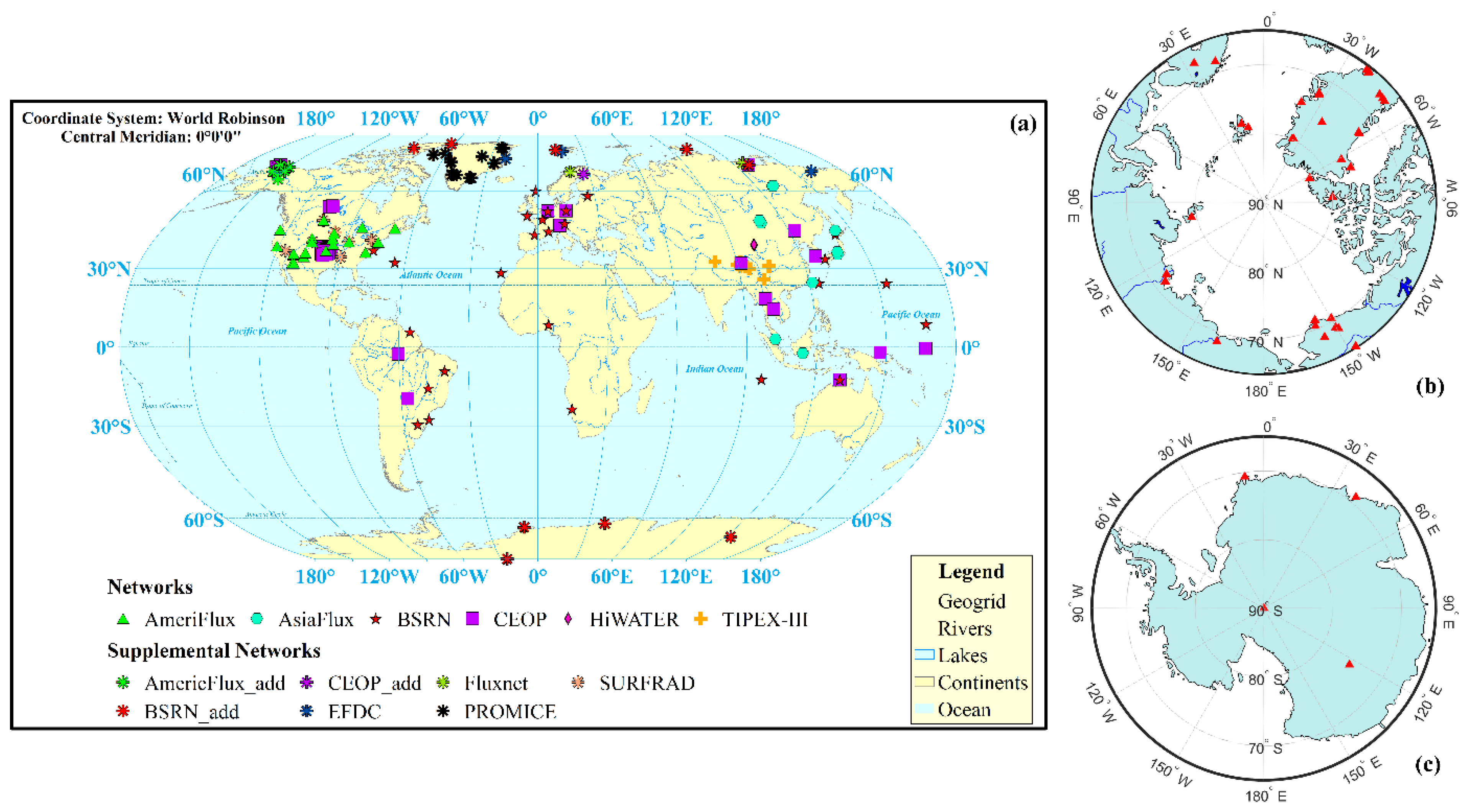
Figure 1. Spatial distribution of the employed flux sites. (a) Site map of observations of surface longwave radiation. (b) Distribution map of observation sites at the North Pole (latitude above 65°N) and (c) the distribution of observation sites at the South Pole (latitude above 65°S).
Remotesensing 15 02955 g001
Figure 2. Validation results for GLASS surface LW radiation under clear-sky and cloudy-sky conditions. (a,b) for GLASS SLUR, (c,d) for GLASS SLDR.
Remotesensing 15 02955 g002
Figure 3. Overall accuracies of the GLASS, CERES-SYN and ERA5 surface LW radiation under all-sky conditions, respectively. (a,b) for the GLASS, (c,d) for the CERES-SYN, and (e,f) for the ERA5.
Remotesensing 15 02955 g003
Figure 4. Differences between the GLASS and ERA5 SLDR at the DRA site in the SURFRAD network. (a): Differences between the GLASS and ERA5 SLDR for Case 1. (b): Similar to (a), but for Case 2. (c): Similar to (a), but for Case 3. (df): Corresponding frequency histograms for (ac), respectively. Unit: W/m2. (g): Information on the GLASS QCs for Case 2.
Remotesensing 15 02955 g004
Figure 5. Biases of the SLUR and SLDR for GLASS (1 km), CERES SYN (0.25°) and ERA5 (1°) at each site. Unit: W/m2.
Remotesensing 15 02955 g005aRemotesensing 15 02955 g005b
Figure 6. Stds of the SLUR and SLDR for GLASS (1 km), CERES SYN (0.25°) and ERA5 (1°) at each site. Unit: W/m2.
Remotesensing 15 02955 g006
Figure 7. RMSEs of the SLUR and SLDR for GLASS (1 km), CERES SYN (0.25°) and ERA5 (1°) at each site. Unit: W/m2.
Remotesensing 15 02955 g007aRemotesensing 15 02955 g007b
Figure 8. Evaluation results of the ERA5 and CERES SYN LW radiation products using the bias-corrected GLASS surface LW radiation product.
Remotesensing 15 02955 g008
Figure 9. Spatial distribution of the global annual mean SLUR and SLDR calculated from GLASS (5 km), CERES SYN (1°) and ERA5 (0.25°) from 2003 to 2020.
Remotesensing 15 02955 g009aRemotesensing 15 02955 g009b
Figure 10. Annual change rate of the GLASS (5 km), CERES SYN (25 km) and ERA5 (100 km) land and ocean SLDR from 2003 to 2020. The pixels marked with a dot indicate their statistical significance (p-values < 0.05) based on the M-K test.
Remotesensing 15 02955 g010
Figure 11. Temporal variation in the annual mean surface LW radiation over the globe, land and ocean.
Remotesensing 15 02955 g011aRemotesensing 15 02955 g011b
Figure 12. Seasonal variation in annual mean SLUR of the Southern and Northern Hemispheres.
Remotesensing 15 02955 g012aRemotesensing 15 02955 g012b
Figure 13. Seasonal variation in the annual mean SLDR in the Southern and Northern Hemispheres.
Remotesensing 15 02955 g013
Table 1. Selected flux sites from 10 flux networks.
No.NetworkNo. of SitesTime Resolution (min)URL
1AsiaFlux1030http://asiaflux.net/, accessed on 1 June 2023
2AmeriFlux4030https://ameriflux.lbl.gov/, accessed on 1 June 2023
3BSRN351https://bsrn.awi.de/, accessed on 1 June 2023
4CEOP4130https://www.eol.ucar.edu/field_projects/ceop, accessed on 1 June 2023
5EFDC260http://www.europe-fluxdata.eu/, accessed on 1 June 2023
6FluxNet230https://fluxnet. fluxdata.org/, accessed on 1 June 2023
7HiWATER-MUSOEXE1910https://data.tpdc.ac.cn/zh-hans/, accessed on 1 June 2023
8PROMICE1460http://www.promice.org/, accessed on 1 June 2023
9SURFRAD71https://gml.noaa.gov/grad/surfrad/index.html, accessed on 1 June 2023
10TIPEX-III1110http://123.56.215.19/tipex, accessed on 1 June 2023
Table 2. Case descriptions and spatial details for GLASS and ERA5.
CaseDescription
Case 1 (clear sky)The cloud QCs of all GLASS SLDR pixels in 25 km are equal to 3, and the cloud amount of the ERA5 grid is 0
Case 2 (partly cloudy sky)Broken clouds in ERA5 with the cloud amount between 0.05~1, and the corresponding GLASS QCs may be equal to 0, 1, 2 and 3 in 25 km
Case 3 (cloud sky)The cloud QCs of all GLASS SLDR pixels in 25 km are controlled to 0, and the cloud amount of ERA5 is 1
Disclaimer/Publisher’s Note: The statements, opinions and data contained in all publications are solely those of the individual author(s) and contributor(s) and not of MDPI and/or the editor(s). MDPI and/or the editor(s) disclaim responsibility for any injury to people or property resulting from any ideas, methods, instructions or products referred to in the content.

