Article

3D Point Cloud Object Detection Algorithm Based on Temporal Information Fusion and Uncertainty Estimation

1
College of Electrical and Control Engineering, North China University of Technology, Beijing 100144, China
2
College of Information, North China University of Technology, Beijing 100144, China
*
Author to whom correspondence should be addressed.
Remote Sens. 2023, 15(12), 2986; https://doi.org/10.3390/rs15122986
Submission received: 21 March 2023 / Revised: 25 May 2023 / Accepted: 6 June 2023 / Published: 8 June 2023
(This article belongs to the Special Issue Signal Processing and Machine Learning for Autonomous Vehicles)

Abstract

:
In autonomous driving, LiDAR (light detection and ranging) data are acquired over time. Most existing 3D object detection algorithms propose the object bounding box by processing each frame of data independently, which ignores the temporal sequence information. However, the temporal sequence information is usually helpful to detect the object with missing shape information due to long distance or occlusion. To address this problem, we propose a temporal sequence information fusion 3D point cloud object detection algorithm based on the Ada-GRU (adaptive gated recurrent unit). In this method, the feature of each frame for the LiDAR point cloud is extracted through the backbone network and is fed to the Ada-GRU together with the hidden features of the previous frames. Compared to the traditional GRU, the Ada-GRU can adjust the gating mechanism adaptively during the training process by introducing the adaptive activation function. The Ada-GRU outputs the temporal sequence fusion features to predict the 3D object in the current frame and transmits the hidden features of the current frame to the next frame. At the same time, the label uncertainty of the distant and occluded objects affects the training effect of the model. For this problem, this paper proposes a probability distribution model of 3D bounding box coordinates based on the Gaussian distribution function and designs the corresponding bounding box loss function to enable the model to learn and estimate the uncertainty of the positioning of the bounding box coordinates, so as to remove the bounding box with large positioning uncertainty in the post-processing stage to reduce the false positive rate. Finally, the experiments show that the methods proposed in this paper improve the accuracy of the object detection without significantly increasing the complexity of the algorithm.

1. Introduction

In the field of autonomous driving, 3D point cloud object detection has garnered significant attention due to its potential to enhance the safety and efficiency of autonomous vehicles by effectively detecting traffic objects in complex environments. Although the data captured by the LiDAR sensors are continuous in time, and a publicly available LiDAR multi-frame sequence dataset [1,2] exists, most 3D object detection algorithms only consider frame-by-frame detection. Compared with only processing single-frame 3D point cloud data, the temporal 3D point cloud object detection algorithm can obtain more complete object structure and location information by using the motion state and historical trajectory of the object to detect the object more accurately.
To better leverage the temporal information of multi-frame point clouds and improve the performance of the 3D point cloud object detector, this paper proposes an algorithm that fuses temporal information through the GRU [3] (gated recurrent unit), as shown in Figure 1. The GRU is designed to fuse the object feature information extracted from the previous frames, with the fusion feature helping to improve object detection in the current frame. The temporal point cloud is taken as the input, and the GRU is used to combine the features of the current frame point cloud with the hidden features of the previous frames. This process enables object detection of the current frame while updating the hidden features of the next frame. In addition, the point cloud data in automatic driving scenarios typically exhibit complex geometric structures and temporal characteristics. In order to enhance the model’s adaptability to the point cloud data, this paper proposes an adaptive GRU model called the Ada-GRU. By introducing an adaptive activation function [4], the Ada-GRU can automatically adjust its gating mechanism to better capture the temporal and geometric information of the point cloud data. The experiments show that this approach can improve detection accuracy. Since we only transfer the high-scoring hidden features to the next frame (red in Figure 1), compared with the method of directly stitching the original point cloud to the adjacent frames [5,6], the proposed method in this paper can also achieve better memory efficiency.
LiDAR point cloud object detection datasets are typically labeled using manual or semi-automatic annotation, which includes information such as the object location and category. Due to the negligence of the annotators, the inaccuracy of semi-automated annotation tools, and other reasons, the point cloud datasets have fuzzy and inaccurate labels. As an example, consider the nuScenes [2] dataset, in which the labels of the two adjacent frames do not match (as shown in Figure 2a). Due to the complexity of the autonomous driving environment, the inherent properties of the LiDAR sensors may cause the acquired point cloud data to be unable to reflect the complete information of the object. When different people make labels, they need to estimate the shape and position of the object subjectively. However, incomplete LiDAR observations may have potential ground-truth bounding boxes of different sizes, shapes, and orientations (as shown in Figure 2b). As a result, label uncertainty is often present in the labels of the LIDAR point cloud datasets, particularly for distant and severely occluded labels. This uncertainty significantly affects the learning process of the 3D point cloud object detection model.
A large number of studies in the field of natural language processing and computer vision demonstrated a positive correlation between the quality of the labels and the robustness of the models [7,8,9]. At present, the state-of-the-art 3D object detectors are usually researched on the premise of a deterministic model, which ignores the impact of label uncertainty. To enhance the accuracy of detecting long-distance and heavily occluded objects, this paper proposes an algorithm that accounts for the uncertainty of bounding box localization by incorporating ideas from uncertainty in deep learning [10,11,12]. Firstly, assuming that the bounding box coordinates follow a Gaussian distribution, the Gaussian distribution function is used to establish the bounding box localization model, where the variance of the Gaussian distribution represents the uncertainty of the corresponding bounding box localization. The larger the Gaussian distribution variance of the coordinates, the higher the uncertainty of the corresponding coordinates, and the lower the confidence. Then, we design a bounding box loss function that enables the network to learn more discriminative features. A new comprehensive scoring rule is designed to remove the bounding box with relatively high localization uncertainty and make the detection results more accurate. Finally, the experimental results show that the detection accuracy of the model is improved under the premise of not significantly increasing the amount of calculations and network parameters.

2. Related Work

2.1. 3D Point Cloud Object Detection

At present, 3D point cloud object detection methods are mainly divided into two categories, point-based and voxel-based. The point-based method takes the original point cloud as the input of the detector, which can better retain the geometric and topological information in the point cloud. By iteratively sampling and grouping, the feature set of the point cloud is extracted, and object detection is then performed [13,14]. The main limitation of the representative point-based method is the grouping operation [15], where the nearest neighbor search operation following the farthest point sampling [16] greatly restricts the inference efficiency of these methods. Voxel-based methods divide the point cloud into a uniform grid for voxelization, and then the 3D convolutional neural network is used for feature extraction to achieve object detection [17]. The advanced voxel-based methods [18,19] use sparse 3D convolution instead of 3D convolution to solve the problem of memory consumption, and a large amount of computation is caused by empty voxels. However, voxelization inevitably leads to information loss and affects detection accuracy. In general, the point-based methods can better retain geometric and topological information, but the calculation speed is slow. Although the voxel-based methods ignore some details, their calculation speed is generally faster. Considering the requirement of real-time performance in practical applications, this paper selects the voxel-based PointPillars [20] object detection algorithm as the baseline.

2.2. Temporal 3D Point Cloud Information Fusion

The temporal 3D point cloud object detection algorithm refers to detecting and recognizing objects in a series of continuous 3D point cloud data. The temporal sequence information fusion is the key to temporal sequence 3D point cloud object detection. WYSIWYG [5] directly splices the original point cloud data of continuous frames and aligns them with point cloud registration methods such as Bayesian filtering to enhance the information of the current frame. MeteorNet [6] proposes direct grouping and chain grouping to aggregate the neighborhood information of each point in the temporal sequence and uses MLP (multi-layer perceptron) to learn the features of each point in the neighborhood. Starnet [21] divides the region of interest in the current frame by using the detection result of the previous frame as prior knowledge, and improves the detection of the current frame by using the selective context aggregation mechanism. FaF [22] proposed a late fusion method, which uses temporal 3D ConvNet (convolution network) for the fusion of point cloud sequences and reduces the sampling of features in the time domain. The above methods ignore the complex spatio-temporal dependence between the different frames of the automatic driving scenarios, which cannot process long-term sequences with multi-frame labels as it lacks the ability to capture complex time features. Additionally, the fusion mode is easily affected by environmental conditions, sensor noise, and other factors. RNNs (recurrent neural networks) and their variants (e.g., LSTM (long short-term memory), GRU, and GatedRNN) have shown good performance in 3D video object detection by leveraging recurrent structures [23,24,25] to acquire temporal features. At present, some studies use RNNs to process the temporal sequence information of point clouds and fuse feature levels. PointRNN [26] employs 3D CNN (convolutional neural network) to extract the local features of each point and send them into LSTM, which processes the multi-frame point cloud features and predicts the scene flow. PillarFlow [27] utilizes LSTM to model the trajectory of the object, predicts its position in the current frame based on the object position information of the previous several frames, and utilizes the motion information of the object to improve the detection performance.

2.3. Uncertainty Estimation

The traditional object detection methods usually assume that the labels are definite, which means that the labels in the training set are all correct. However, in practical applications, the labels are often uncertain due to the error of human labeling, noise in the dataset, and other factors. The uncertainty labels affect the model’s learning and may lead to the object detection algorithm giving the wrong bounding box coordinates. To solve this problem, some researchers try to introduce uncertainty estimation into deep learning for object detection algorithms. The common modeling methods of uncertainty estimation include Bayesian deep learning [28], the Gaussian process [29], and so on. Feng et al. [12] used the Monte Carlo dropout technique to obtain an a posteriori distribution of the model output by sampling the model multiple times and were able to capture the uncertainty of the model. Timm et al. [30] introduced heteroscedastic aleatoric uncertainties to optimize the mean and variance of the network during training so that the model could adapt to different scenarios. The above methods can obtain the estimated value of the uncertainty by modeling so as to improve the accuracy and robustness of the object detection model. Meanwhile, the uncertainty estimation results can also be applied to conduct sample screening, model selection, and other operations, so as to improve the performance of the object detection model.

3. Approach

In this work, the 3D point cloud object detection algorithm that utilizes temporal information fusion and uncertainty estimation is proposed. The overall framework of the algorithm is introduced in Section 3.1. To improve the detection accuracy, the algorithm uses a temporal sequence information fusion method based on the Ada-GRU, as explained in Section 3.2. We also propose a probability distribution model that considers the uncertainty of the bounding box coordinate positioning, which is described in Section 3.3. Additionally, Section 3.4 introduces the corresponding object composite score, and Section 3.5 introduces a new loss function.

3.1. Framework

The framework of the method is shown in Figure 3. Firstly, the backbone extracts the feature of the current frame point cloud data x t , which are represented by x t . Then, the current frame’s feature x t and the previous frames’ hidden feature h t 1 are jointly voxelized [31] to compensate for the inter-frame ego-motion. This means that the hidden feature h t 1 of the previous frames is converted to the coordinate system of the current frame and is denoted as h t 1 . Both h t 1 and x t are input into the Ada-GRU for inter-frame feature screening and processing, and the hidden feature h t of the current frame is output. The hidden feature is input into the object detection head to generate the 3D object proposal of the current frame. At the same time, the uncertainty of the bounding box coordinate position is estimated. The Gaussian distribution function is used to establish a probability distribution model of the bounding box coordinates. The model predicts the Gaussian distribution mean and variance of each coordinate component of the bounding box. The mean represents the predicted value of the coordinate component, while the variance represents the localization uncertainty of each coordinate component. Finally, a new method for computing the object’s comprehensive score is proposed. The corresponding loss function is designed to optimize both the location uncertainty and the predicted value of the bounding box localization at the same time so as to improve the accuracy of the algorithm’s prediction of the bounding box localization.

3.2. Temporal Information Fusion

The GRU is an improvement on LSTM and is one of the variants of the RNN (recurrent neural network). The RNN is a type of neural network that can handle sequential data. In the traditional RNN model, the current input and the previous time step’s state are combined through a recurrent unit to generate a new state. However, this structure is prone to the issues of vanishing and exploding gradients, which limits the long-term dependency capability of RNNs. LSTM, on the other hand, addresses these problems by introducing memory cells and gate mechanisms, enabling a better handling of long sequential data. In comparison to the LSTM model, the GRU removes one gate unit, resulting in fewer model parameters and a lighter model overall. This makes the GRU more practical in certain application scenarios, such as autonomous driving. The main idea of the GRU is the introduction of the gating mechanism, which controls the flow of information and selectively forgets past information while updating the information at the current time. The GRU model includes two key parts, which are the reset gate and the update gate. The reset gate controls the degree of influence for the information in the past to the present moment. Additionally, the update gate controls the degree of update for the new information in the present moment and the information in the past moment. In addition, the GRU also introduces a hidden state to save information from previous moments, which can be reused in future moments. The traditional GRU typically uses the sigmoid and tanh functions as the activation functions for the gating mechanism, and their parameters are fixed. However, when dealing with point cloud data with complex distributions, these fixed-parameter activation functions may not fully adapt to the data’s characteristics. To address this issue, this article proposes the Ada-GRU. In the Ada-GRU, the activation function’s parameters are learned through training, enabling the model to adaptively adjust the gating mechanism based on the input data’s characteristics. This adaptability allows the model to better capture the temporal and geometric information within the point cloud data.
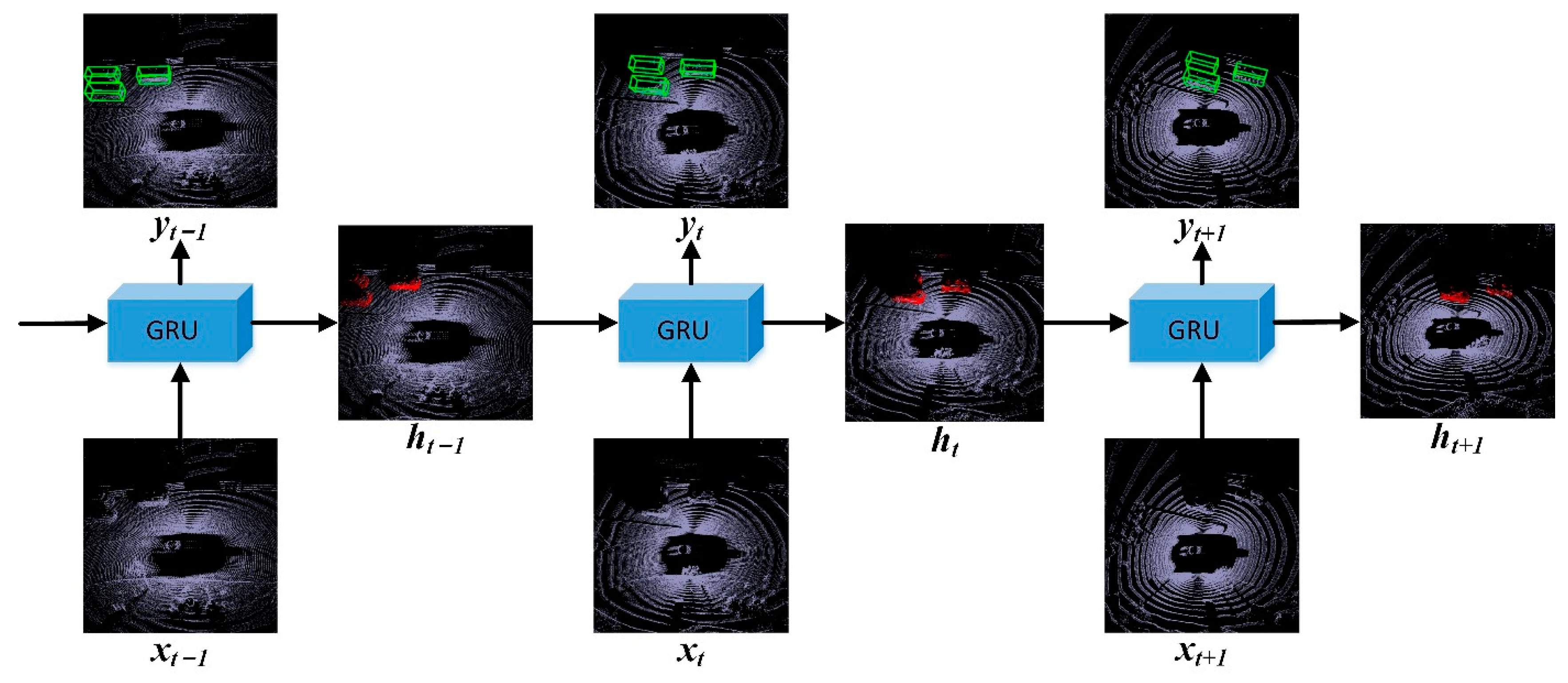
Ada-GRU: The Ada-GRU model is used to fuse the characteristics of the temporal sequence of the LiDAR point cloud frames, and the model structure and basic notation are shown in Figure 4. In the figure, h t 1 represents the hidden features of the previous frames, accumulating the historical information over the temporal sequence. By utilizing the historical information, h t 1 can provide a more comprehensive understanding of the point cloud frame at the current moment, enabling the model to better capture the dynamic changes and motion characteristics of the object. r t is the parameter of the reset gate, which has a value in the range of ( 0 ,   1 ) and serves as a scaling factor that controls how much information is retained by the hidden feature h t 1 of the previous frames. The calculation method is as follows:
r t = σ ( W r [ h t 1 , x t ] + b r )
where W r represents the weight matrix of the reset gate, [ h t 1 , x t ] represents the concatenation of the hidden feature h t 1 of the previous frames and the feature x t of the current frame based on the feature dimension, “ ” represents the matrix multiplication operation, and b r represents the bias vector of the reset gate. σ represents the following adaptive sigmoid function:
σ ( x ) = 1 1 + e α x
which restricts the reset gate parameter r t within the range of ( 0 ,   1 ) . In comparison to the traditional sigmoid function, the adaptive sigmoid function introduces a trainable parameter α , which can learn to adjust the slope of the sigmoid function. Figure 5 (left) shows the variations in the slope when different values of α are used. When α is larger, the sigmoid function exhibits a steeper change curve, making the gating unit easier to “open” or “close”. Conversely, when α is small, the change curve of the sigmoid function becomes gentler, resulting in smoother responses of the gated units to the sequence features. By introducing the adaptive sigmoid function, the model can automatically adjust the gating mechanism according to the characteristics of the data, thereby enhancing the fusion performance of the temporal sequence information in the point cloud data. After obtaining the reset gate parameter r t , it is multiplied with the previous frames’ hidden feature h t 1 to retain the relevant information for the current frame. Then, it is concatenated with x t based on the feature dimension, and the candidate hidden feature h is calculated as follows:
h = t h ( W h [ r t h t 1 , x t ] + b h )
where W h is the weight matrix of the candidate hidden feature, “ ” represents the element-wise multiplication operation, b h represents the bias vector, and t h represents the following adaptive hyperbolic tangent function:
t h ( x ) = e β x e β x e β x + e β x
of which its effect is to perform a nonlinear transformation and restrict the candidate hidden feature h within the range of ( 1 ,   1 ) . Similar to the adaptive sigmoid function, the slope of the hyperbolic tangent function is adjusted by introducing the trainable parameter β . Figure 5 (right) shows the variations in the slope when different values of β are used. The main purpose of the hidden feature h is to incorporate both the feature x t of the current frame and the hidden feature h t 1 of the previous frames into the current frame. The candidate hidden feature h can be seen as a way to remember the “state” of the point cloud feature in the current frame.
Finally, during the “update memory” phase of the Ada-GRU, the update gate parameter z t is calculated as follows:
z t = σ ( W z [ h t 1 , x t ] + b z )
where W z represents the weight matrix of the update gate, and b z represents the bias vector. The update gate parameter z t is used to control the influence of the previous frames’ hiding feature h t 1 and the current frame’s candidate hidden feature h on the current frame’s hidden feature h t . The hidden feature h t of the current frame is the output of the Ada-GRU model, and its calculation method is as follows:
h t = ( 1 z t ) h t 1 + z t h
where ( 1 z t ) h t 1 represents the influence of the previous frames’ hidden features on the current frame, and z t h represents the influence of the current frame’s candidate hidden features on the current frame. By using the update gate parameter z t to control the weighted sum of the previous frames’ hidden features and the current frame’s hidden features, the Ada-GRU model can flexibly regulate the influence of the previous frames’ hidden features on the current frame. This enables the model to effectively capture the temporal feature information of the point cloud.

3.3. Localization Uncertainty

After fusing the temporal features of the point cloud, the detection head is used to generate 3D object proposals for the current frame. The SSD detection head [20] is commonly used, which can predict the center location ( i . e . ,   b x ,   b y ,   and   b z ) , the size ( i . e . ,   b w ,   b l ,   and   b h ) , the orientation b θ , the category score ( i . e . ,   P 1 ,   P 2 P C ) , and the direction scores ( i . e . ,   d i r 1   and   d i r 2 ) for the bounding box (shown in Figure 6a). However, the SSD detection head does not provide the prediction for the scores of the bounding box coordinates, so the uncertainty for the bounding box coordinates’ localization cannot be obtained.
In order to obtain the uncertainty of the 3D bounding box coordinates’ localization, it is necessary for the detection head to predict both the bounding box coordinates and the probability distribution of those coordinates. In this paper, the Gaussian distribution function is used to re-model the bounding box coordinates, where each bounding box coordinate predicted by the detection head is modeled as the mean and variance, the mean value represents the predicted bounding box coordinates, and the variance represents the uncertainty of the coordinate positioning. As shown in Figure 6b, the output of the detection head consists of seven coordinate components (i.e., b x ,   b y ,   b z ,   b w ,   b l ,   b h , and b θ ) of the bounding box and the corresponding localization uncertainty scores (i.e.,   σ ^ b x 2 ,   σ ^ b y 2 ,   σ ^ b z 2 ,   σ ^ b w 2 ,   σ ^ b l 2 ,   σ ^ b h 2 , and σ ^ b θ 2 ), where b x , b y , and b z represent the coordinates of the center point of the 3D bounding box; b w ,   b l , and b h represent the size of the bounding box; and b θ represents the orientation of the bounding box. According to the structure of the SSD detection head’s output layer, the bounding box coordinates and the corresponding localization uncertainty score are transformed as follows:
μ b x = sigmoid ( b x ) ,   μ b y = sigmoid ( b y ) , μ b z = sigmoid ( b z ) , μ b θ = sigmoid ( b θ )
μ b w = b w , μ b l = b l , μ b h = b h
σ b x 2 = sigmoid ( σ ^ b x 2 ) , σ b y 2 = sigmoid ( σ ^ b y 2 ) , σ b z 2 = sigmoid ( σ ^ b z 2 ) , σ b θ 2 = sigmoid ( σ ^ b θ 2 )
σ b w 2 = e σ ^ b w 2 , σ b l 2 = e σ ^ b l 2 , σ b h 2 = e σ ^ b h 2
The purpose of using the sigmoid function in Formula (7) is normalization, which maps the center point and orientation to the range of ( 0 ,   1 ) . This ensures a consistent scale and enables the adaptation to the Gaussian distribution modeling. Meanwhile, in Formula (9), the variances of the center point and orientation are also mapped to the range of (0, 1). Since the size of the predicted bounding box can be any value between ( , + ) , in order to retain the flexibility of the size prediction of the bounding box, it is not normalized in Formula (8). Meanwhile, in Formula (10), the uncertainty score of the bounding box size is mapped to the range of ( 0 , + ) using a natural exponential function to ensure that the uncertainty score is positive.
The Gaussian probability density function for predicting the bounding box coordinates is as follows:
P ( α μ , σ 2 ) = 1 2 π σ 2 e ( α μ ) 2 2 σ 2
where μ is the mean value, σ 2 is the variance, and α is the possible value of each coordinate component of the bounding box. The seven coordinate components (i.e., μ b x ,   μ b y ,   μ b z ,   μ b w ,   μ b l ,   μ b h , and μ b θ ) of the transformed coordinates and the corresponding variances of the Gaussian distribution (i.e., σ b x 2 ,   σ b y 2 ,   σ b z 2 ,   σ b w 2 ,   σ b l 2 ,   σ b h 2 , and σ b θ 2 ) are substituted into the above formula, respectively, to obtain the probability distribution of the seven coordinate components. Figure 7 illustrates an example of the model’s prediction for the bounding box coordinate component. The horizontal axis represents the value of the coordinate component, and the vertical axis represents the probability density. L1 and L2 are the two Gaussian probability density function curves predicted by the detection head. Each curve represents the probability density when the coordinate component takes any value of α . When α is equal to the predicted value μ (L3) of the coordinate component, the probability density reaches its maximum. In addition, when α is ground-truth, its probability density value can reflect the prediction error. For example, the predicted values of L1 and L2 are both 0.3, while the variance of the L1 prediction is relatively large, and the uncertainty of the L1 prediction coordinates is relatively large. When the ground-truth value is 0.4 (L4), there is a significant difference with the predicted value, indicating a higher level of uncertainty, and it is evident that the prediction error of L1 should be smaller than that of L2 in the calculation. By calculating the error between the predicted value and the ground-truth (both 0.1), it is impossible to distinguish whether L1 or L2 is better. However, the probability density can distinguish between them. This property of the probability density function can be utilized in the calculation of the loss, as discussed in Section 3.5.

3.4. Object Comprehensive Score

After obtaining the Gaussian distribution variances representing the positioning uncertainty of the seven coordinate components for the prediction bounding box, the localization uncertainty U b o x of the prediction bounding box is calculated by the positioning uncertainties of each coordinate component as follows:
U b o x = σ b x 2 × σ b y 2 × σ b z 2 × σ b w 2 × σ b l 2 × σ b h 2 × σ b θ 2 δ
The bounding box localization score S b o x is calculated based on the bounding box localization uncertainty. The S b o x is negatively correlated with the U b o x as follows:
S b o x = e U b o x
In Formula (12), δ is a hyperparameter used to adjust the uncertainty of the bounding box positioning. In the experimental part, when testing the trained model, it is found that the value range of σ b x 2 × σ b y 2 × σ b z 2 × σ b w 2 × σ b l 2 × σ b h 2 × σ b θ 2 is mainly distributed in the range of ( , 10 7 ) . Therefore, we set the value of the hyperparameter δ to be 10 8 , distributing the value of the U b o x in the range of ( 0 ,   10 ) as much as possible; this can effectively avoid the exponential function overflow of Formula (13) so as to ensure the stability of the S b o x . In the post-processing stage of the point cloud object detection, the bounding box localization score S b o x and the object classification score S o b j are used to calculate the comprehensive score S of the object as follows:
S = S b o x × S o b j
In the post-processing stage of the 3D point cloud object detection, a threshold is generally set. The bounding box with scores lower than the threshold are filtered out. If the candidate boxes are only screened based on the classification score, it may lead to a false positive because some candidate boxes may have a high classification score S o b j , but their positions and sizes differ greatly from the actual object box. Therefore, the proposed bounding box localization score S b o x can reduce the comprehensive score S of objects with a high bounding box localization uncertainty, causing it to be lower than the threshold, and thus, filtered out. This helps to reduce false positives and improve the detection accuracy.

3.5. Loss-Function

Applying the Gaussian distribution function to model the bounding box coordinates requires the redesign of the bounding box loss function. This allows the model to simultaneously optimize both the predicted value of the 3D bounding box coordinates and the localization uncertainty during the training process. By substituting the ground-truth coordinate into Formula (11), the corresponding probability density value can be obtained. This value can then be used to assess the accuracy of the prediction result. The higher the probability density value, the more accurate the prediction result is considered to be. Therefore, this paper adopts the negative logarithmic likelihood loss design method [11]. The total localization loss l o c is calculated for the predicted values of the bounding box coordinate components. The calculated method is as follows:
l o c = c ( x , y , z , w , l , h , θ ) λ × ln ( tanh ( P ( g b c | μ b c , σ b c 2 ) + ε ) ) × I o b j
where g b c is the label value (ground-truth) of each coordinate component of the bounding box. Because the Gaussian probability density value may be greater than one, the hyperbolic tangent function is used to ensure a non-negative loss value for the bounding box. This helps to improve the stability of the network. ε is an error limit that is set to 10 7 to prevent infinite loss values. I o b j indicates whether the anchor box at the corresponding position is responsible for detecting the current object. It takes a value of 1 if it is responsible for detecting the current object, and a value of 0 otherwise. In order to increase the loss weight for smaller objects, the following coefficient λ is introduced:
λ = 2 g w × g l × g h
where g w , g l , and g h represent the width, length, and height, respectively, of the ground-truth bounding box after normalization with respect to the original point cloud. For the predicted discretized direction loss d i r and object classification loss, the calculation is the same as that obtained using PointPillars [20]. Therefore, the total loss is obtained by using the following equation:
= 1 N p o s ( β l o c l o c + β c l s c l s + β d i r d i r )
where N p o s is the number of positive anchors. For the hyperparameters, we follow the common settings of β l o c = 2 , β c l s = 1 , and β d i r = 0.2 of the 3D point cloud object detection algorithm [18,20].

4. Experimental Results

4.1. Datasets

The nuScenes dataset is a large-scale autonomous driving dataset designed for 3D object detection in urban scenes. It contains 1000 driving sequences, each lasting 20 s. The dataset is divided into 700 training scenarios, 150 verification scenarios, and 150 test scenarios. The nuScenes dataset consists of LiDAR point cloud data collected at a frequency of 20 Hz. The LiDAR sensor used in the dataset is a 32-channel LiDAR, which captures around 30,000 points per frame. The dataset provides annotations for 10 classes of objects, and the annotations include 3D bounding box information for each object. The main evaluation metrics of the dataset are the mAP (mean average precision) [32] and NDS (nuScenes detection score) [2]. These metrics are used to evaluate the performance of the proposed temporal sequence 3D object detection method in this paper on the nuScenes validation set. The mAP is calculated based on the AP (average precision) of the different object classes, where a match is determined by thresholding the 2D center distanced on the ground plane. The NDS is the weighted average of the mAP and other attribute measures, including location, size, orientation, velocity, and others.

4.2. Implementation Details

Baseline. PointPillars [20] efficiently processes the point cloud data by using the voxel-based vertical division and 2D convolutional neural network. This approach is well suited for real-time requirements in autonomous driving scenarios. However, the official codebase (https://github.com/nutonomy/second.pytorch, accessed on 25 November 2022) only supports the KITTI dataset, which lacks continuous frames. In order to reproduce PointPillars using the nuScenes dataset, this paper uses another codebase (https://github.com/traveller59/second.pytorch, accessed on 25 November 2022) recommended by the authors of PointPillars and adopts it as the baseline for the experiments.
Training. The training includes two stages. In the first stage, the same architecture as PointPillars is employed to jointly train the VFE (voxel feature encoding), backbone, and detection head of the single-frame detector. The detection ranges for the X-axis and the Y-axis are set to (−51.2 m, 51.2 m), while the detection range for the Z-axis is (−5 m, 3 m), and the voxel size is (0.2 m, 0.2 m, 8 m). Using the one-cycle policy [33] to train the model with 20 epochs, the maximum learning rate is set to 3 × 10⁻³. In the second stage, on the basis of the single-frame detector, the temporal sequence information fusion module is added to train the multi-frame detector. To achieve a good balance between the performance and the complexity, the number of frames for the temporal fusion is set to four. Firstly, the model is initialized with the weights obtained from the first training stage. The feature extraction backbone is then frozen, and the temporal sequence information fusion module is trained. The training process consists of 20 epochs using the one-cycle strategy, with a maximum learning rate of 1 × 10⁻³. Then, the backbone is unfrozen to fine-tune the entire network. This fine-tuning process involves training for 10 epochs with the same learning rate scheduling strategy, where the maximum learning rate is set to 1 × 10⁻⁴. The training was conducted over a span of five days using two NVIDIA Quadro RTX 6000 GPUs. The AdamW [34] optimizer was used with a batch size of eight (four frames per GPU).

4.3. Quantitative Evaluation

Ablation experiment A. The improvement of the baseline detection accuracy by the two methods proposed in this paper are shown in Table 1. In the table, the method based on the Ada-GRU for the temporal sequence information fusion is denoted by “T”, and the detection head with the localization uncertainty estimation is denoted by “U”. The last two columns of Table 1 show that both methods proposed in this paper lead to improvements in the baseline detection accuracy (both the mAP and NDS improved). In order to better understand the work in this paper, we divided the objects in the nuScenes validation set into the following three subsets based on their distances from the sensor: (<15 m), (15–30 m), and (>30 m). The accuracy assessment on the different subsets are shown in columns 4–6 of Table 1. By comparing the data in the second and third rows of Table 1, it can be seen that the temporal sequence information fusion method based on the Ada-GRU significantly improves the detection accuracy of objects within the range of (15~30 m) and (>30 m). The method achieves gains of 6.1% and 6.3%, respectively. It indicates that the temporal sequence information fusion is helpful for detecting objects at medium and long distances. The main reason is that the shape information of objects at medium and long distances is relatively blurry. The reset gate and update gate mechanisms of the Ada-GRU can effectively utilize the cumulative effect of the multi-frame point cloud data to acquire rich object motion information, thereby enhancing the object detection performance. By comparing the data in the second and fourth rows of Table 1, it can be observed that the detection accuracy of the objects in the range of (>30 m) is significantly improved when using the detection head with the localization uncertainty estimation, achieving a gain of 4.3%. This result indicates that as the distance increases, the uncertainty of the bounding box also increases, and the role of the positioning uncertainty estimation in the detection head becomes more significant. The main reason is that the detection head containing the localization uncertainty estimation can provide a probability distribution for each bounding box and provide the localization uncertainty score. By fusing the localization uncertainty score and the object classification score, the bounding boxes with greater uncertainty can be filtered out in the post-processing stage, and more accurate object detection results can be obtained. By comparing the second and fifth rows of Table 1, it can be seen that the algorithm achieves the highest detection accuracy when the two methods are used together, indicating their compatibility.
Table 2 shows the improvement in the baseline performance of the proposed method in the nuScenes dataset, including the AP for each category. The results indicate that the model proposed in this paper has a better detection effect on objects with larger sizes, such as cars and buses, for two reasons. First, objects with larger sizes usually exhibit more stable motion patterns and shape features in the time series data, whereas objects with smaller sizes experience relatively larger changes in position and shape between successive frames, which introduce additional challenges. Second, the larger the object size, the greater the uncertainty in the bounding box coordinates and dimensions, thereby amplifying the benefits of the uncertainty modeling.
Ablation experiment B. Table 3 shows the performance improvement achieved by the proposed detection head with the localization uncertainty estimation on the baseline, as well as a comparison with other commonly used single-frame detection algorithms. Among the comparison methods, the same as the baseline, SECOND [18] and CenterPoint [19] are both voxel-based single-frame detection methods that exhibit a higher detection accuracy but also a higher algorithm complexity compared to the baseline. To evaluate the performance, we measured the MACs (multiply accumulate operations) and latency of the algorithm during a single inference on a single RTX 6000 GPU, which provides an indication of the algorithm’s complexity. Compared with the baseline, the proposed method achieves an improvement of 3.1% in the mAP and 4.9% in the NDS, with an increase of approximately 2.1% in the MACs and about 4.4% in the latency. Compared with SECOND, the detection efficiency and accuracy of the proposed algorithm are higher. Compared with CenterPoint, the detection accuracy of the proposed algorithm is slightly lower, but the latency is only 0.4 times that of CenterPoint. The results show that the detection head, which includes the localization uncertainty, does not significantly increase the calculation workload of the detection time. It effectively improves the detection accuracy while maintaining computational efficiency.
Table 4 shows the performance comparison between the proposed algorithm and the state-of-the-art algorithm of the past two years. Compared with Focals Conv and VoxelNeXt, the proposed method exhibits a lower detection accuracy, but it clearly has a lower latency. When compared with CenterPoint, the detection accuracy of the proposed method is close to that of CenterPoint (with a 0.6% lower mAP and a 1.7% higher NDS), but it has a lower latency. Therefore, the advantage of the proposed algorithm is that it achieves a good balance between the detection accuracy and latency.
Ablation experiment C. Table 5 shows the performance improvement achieved by the proposed temporal sequence information fusion method based on the Ada-GRU compared to the baseline. In order to further study the effectiveness of the proposed temporal sequence fusion method, late-fusion models (LFM) in FaF [22] and ConvLSTM in CLN [35] are used for comparison. In these comparisons, the temporal fusion part is replaced, while the other parts are unchanged. Compared to the baseline, the temporal fusion method in this paper (the sixth row of Table 5) achieved an increase of 4.7% in the mAP, and an increase of 4.5% in the NDS. However, this improvement came at the cost of approximately 3% more MACs and approximately 7.1% more latency. The LFM temporal fusion method is inferior to the Ada-GRU method in terms of the accuracy gain and computational complexity. The gain in the detection accuracy of the ConvLSTM temporal fusion method is close to the proposed Ada-GRU method, but the algorithm complexity is slightly higher. Compared to the traditional GRU model, the Ada-GRU achieves higher detection accuracy gains without increasing the algorithm complexity. The experimental results show that the proposed temporal fusion method based on the Ada-GRU achieves a better balance between the algorithm complexity and detection accuracy. This is due to the efficient gating mechanism of the Ada-GRU, and the use of the adaptive activation function instead of the traditional activation function does not add additional computational overhead in the inference phase. The last row of Table 5 shows the effect of using the Ada-GRU in combination with the detection head containing the localization uncertainty estimation. The detection accuracy is the highest among all the comparison methods, and the latency is only 40.3 ms.
Table 4. Comparison with other methods on nuScenes validation split.
TypeMethodmAPNDSLatency (ms)
Single-frameBaseline52.361.334.4
Focals Conv [36]61.268.1159.0
VoxelNeXt [37]60.067.166.0
CenterPoint (voxel size = 0.1) [19]56.064.560.5
Ours55.466.237.1

4.4. Qualitative Results

The visualization result of the 3D point cloud object detection is shown in Figure 8, which shows the impact of our proposed method on the baseline. It can be seen that the 3D point cloud object detection algorithm proposed in this paper has more precise detection results, which is based on the temporal information fusion and location uncertainty estimation. The yellow circles mark the missed detection objects. Comparing our method with the baseline, it is evident that our approach has fewer missed detections. This improvement can be attributed to the utilization of the temporal sequence information fusion, which leverages the object motion state information such as the trajectory and speed to enhance the detection performance. The red circles mark the false positive objects. The main reason for the significant reduction in false positives in our method is the incorporation of the localization uncertainty estimation. This enables the removal of the surrounding boxes with a high localization uncertainty during the post-processing stage, resulting in an improved localization accuracy.

4.5. Additional Experiments

Furthermore, to verify the generalization power of the methods presented in this paper, we conducted experiments on the Waymo dataset [1] by following the default setting in the OpenPCDet (https://github.com/open-mmlab/OpenPCDet, accessed on 20 January 2023) codebase and using 20% of the training data. The performance of the proposed algorithm was comprehensively evaluated at different difficulty levels using the “AP LEVEL 1” and “AP LEVEL 2” evaluation metrics from the Waymo dataset. Table 6 shows the improvement of the baseline method’s detection performance achieved by the proposed algorithm and compares it with the state-of-the-art algorithm from the past two years. The proposed algorithm demonstrates the advantages in terms of a higher detection accuracy and a lower inference latency. Figure 9 shows the visual results, clearly showing the more accurate detection outcomes achieved by the proposed algorithm.
To further evaluate the performance of this paper’s algorithm, we tested it on the NVIDIA Jetson AGX Xavier edge computing device and deployed the model using TensorRT. In order to reduce the contingency, we started to count the performance data from frame 20 and calculated the average value. Table 7 shows the resource utilization and power consumption of the algorithm during operation, while Table 8 shows the inference delay of each module of the algorithm. According to the test results, the total inference delay of the proposed algorithm on the Jetson Xavier AGX is 73 ms. When the frame rate of the LiDAR sensor is 10 Hz, our algorithm can achieve real-time operation, which is suitable for use in autonomous driving scenarios.

5. Conclusions

Autonomous vehicles have high precision and real-time requirements for the 3D point cloud object detection algorithm. To meet these requirements, this paper studies the 3D point cloud object detection algorithm based on the temporal information fusion and uncertainty estimation. First of all, this paper proposes the Ada-GRU, an adaptive GRU model designed for the temporal information fusion. The Ada-GRU runs in a stream and controls the point cloud features of previous frames to be forgotten or retained by the adaptive gating mechanism, and the retained features assist the current frame in the object detection. The experiments show that the proposed temporal fusion method can effectively improve the model’s detection accuracy for medium- and long-distance objects. Additionally, through the deep research of the point cloud data, it is found that the label of the point cloud data has serious positioning uncertainty, and there may be multiple potential ground-truth bounding boxes for each object. Therefore, based on the uncertainty idea in deep learning, this paper proposes to establish the probability distribution model of the 3D bounding box coordinates through the Gaussian distribution function. This model can predict the coordinates of the bounding box and provide the uncertainty score of the coordinates. The corresponding object comprehensive score and the loss function are designed so that the model can learn and estimate the uncertainty of the bounding box coordinates. The experiment shows that the proposed method can remove the bounding box with large positioning uncertainty in the post-processing stage so as to reduce the false positive rate. Finally, the ablation experiments prove that the two methods proposed in this paper can improve the detection accuracy without significantly increasing the complexity of the baseline algorithm, and the real-time performance is good. In our future work, we plan to extend the temporal fusion method and the idea of positioning uncertainty proposed in this paper to other object detection algorithms so as to further improve the comprehensive performance of 3D point cloud object detection algorithms.

Author Contributions

Conceptualization, G.X. and Y.L.; methodology, G.X. and Y.L.; software, G.X.; validation, G.X. and Y.L.; formal analysis, Y.W.; investigation, H.Q.; resources, H.Q., Y.W. and Y.L.; data curation, G.X.; writing—original draft preparation, Z.L.; writing—review and editing, G.X. and Z.L.; visualization, Y.W.; supervision, H.Q.; project administration, Y.W. and G.X.; funding acquisition, Y.W. and Y.L. All authors have read and agreed to the published version of the manuscript.

Funding

This research was funded by the National Natural Science Foundation of China under grant numbers 62131001 and 61971456, by the General Project of Science and Technology Plan of Beijing Municipal Commission of Education under grant number KM202010009011, and by the Yuyou Talent Training Program under grant number 218051360020XN115/014 of the North China University of Technology.

Data Availability Statement

Not applicable.

Acknowledgments

We thank the anonymous reviewers for their good suggestions and comments to help improve the quality of the paper.

Conflicts of Interest

The authors declare no conflict of interest.

References

  1. Sun, P.; Kretzschmar, H.; Dotiwalla, X.; Chouard, A.; Patnaik, V.; Tsui, P.; Guo, J.; Zhou, Y.; Chai, Y.; Caine, B.; et al. Scalability in perception for autonomous driving: Waymo open dataset. arXiv 2019, arXiv:1912.04838. [Google Scholar]
  2. Caesar, H.; Bankiti, V.; Lang, A.H.; Vora, S.; Beijbom, O. Nuscenes: A multimodal dataset for autonomous driving. In Proceedings of the IEEE/CVF Conference on Computer Vision and Pattern Recognition (CVPR), Seattle, WA, USA, 13–19 June 2020; pp. 11621–11631. [Google Scholar]
  3. Cho, K.; Merrienboer, B.V.; Gulcehre, C.; Bahdanau, D.; Bougares, F.; Schwenk, H.; Bengio, Y. Learning phrase representations using rnn ncoder-decoder for statistical machine translation. In Proceedings of the Conference on Empirical Metods in Natural Language Processing (EMNLP), Doha, Qatar, 25–29 October 2014. [Google Scholar]
  4. Jagtap, A.D.; Kawaguchi, K.; Karniadakis, G.E. Adaptive activation functions accelerate convergence in deep and physics-informed neural networks. J. Comput. Phys. 2020, 404, 109–136. [Google Scholar] [CrossRef] [Green Version]
  5. Peiyun, H.; Jason, Z.; David, H.; Deva, R. What you see is what you get: Exploiting visibility for 3d object detection. In Proceedings of the 2020 IEEE/CVF Conference on Computer Vision and Pattern Recognition (CVPR), Seattle, WA, USA, 13–19 June 2020; pp. 10998–11006. [Google Scholar]
  6. Liu, X.; Yan, M.; Bohg, J. Meteornet: Deep learning on dynamic 3d point cloud sequences. In Proceedings of the IEEE International Conference on Computer Vision (ICCV), Seoul, Republic of Korea, 27 October 2019–2 November 2019; pp. 9245–9254. [Google Scholar]
  7. Zhang, C.; Bengio, S.; Hardt, M.; Recht, B.; Vinyals, O. Understanding deep learning (still) requires rethinking generalization. Commun. ACM 2021, 64, 107–115. [Google Scholar] [CrossRef]
  8. Luengo, J.; Shim, S.O.; Alshomrani, S.; Altalhi, A.; Herrera, F. Cnc-nos: Class noise cleaning by ensemble filtering and noise scoring. Knowl. -Based Syst. 2018, 140, 27–49. [Google Scholar] [CrossRef]
  9. Northcutt, C.; Jiang, L.; Chuang, I. Confident learning: Estimating uncertainty in dataset labels. J. Artif. Intell. Res. 2021, 70, 1373–1411. [Google Scholar] [CrossRef]
  10. Kendall, A.; Gal, Y. What uncertainties do we need in Bayesian deep learning for computer vision? In Proceedings of the 2017 Annual Conference on Neural Information Processing Systems (NIPS), Long Beach, CA, USA, 4–9 December 2017; pp. 5574–5584. [Google Scholar]
  11. Choi, J.; Chun, D.; Kim, H.; Lee, H.J. Gaussian YOLOv3: An accurate and fast object detector using localization uncertainty for autonomous driving. In Proceedings of the 2019 IEEE International Conference on Computer Vision (ICCV), Seoul, Republic of Korea, 27 October 2019–2 November 2019; pp. 502–511. [Google Scholar]
  12. Feng, D.; Rosenbaum, L.; Dietmayer, K. Towards safe autonomous driving: Capture uncertainty in the deep neural network for lidar 3D vehicle detection. In Proceedings of the 2018 International Conference on Intelligent Transportation Systems (ITSC), Maui, HI, USA, 4–7 November 2018; pp. 3266–3273. [Google Scholar]
  13. Shi, S.; Wang, X.; Li, H. Pointrcnn: 3d object proposal generation and detection from point cloud. In Proceedings of the IEEE/CVF Conference on Computer Vision and Pattern Recognition (CVPR), Long Beach, CA, USA, 15–20 June 2019; pp. 770–779. [Google Scholar]
  14. Yang, Z.; Sun, Y.; Liu, S.; Shen, X.; Jia, J. Std: Sparse-to-dense 3d object detector for point cloud. In Proceedings of the IEEE/CVF International Conference on Computer Vision (ICCV), Seoul, Republic of Korea, 27 October–2 November 2019; pp. 1951–1960. [Google Scholar]
  15. Qi, C.R.; Su, H.; Mo, K.; Guibas, L.J. Pointnet: Deep learning on point sets for 3d classification and segmentation. In Proceedings of the IEEE Conference on Computer Vision and Pattern Recognition (CVPR), Honolulu, HI, USA, 21–26 July 2017; pp. 652–660. [Google Scholar]
  16. Yang, Z.; Sun, Y.; Liu, S.; Jia, J. 3dssd: Point-based 3d single stage object detector. In Proceedings of the IEEE/CVF Conference on Computer Vision and Pattern Recognition (CVPR), Seattle, WA, USA, 13–19 June 2020; pp. 11040–11048. [Google Scholar]
  17. Zhou, Y.; Tuzel, O. Voxelnet: End-to-end learning for point cloud based 3d object detection. In Proceedings of the IEEE Conference on Computer Vision and Pattern Recognition (CVPR), Salt Lake City, UT, USA, 18–23 June 2018; pp. 4490–4499. [Google Scholar]
  18. Yan, Y.; Mao, Y.; Li, B. Second: Sparsely embedded convolutional detection. Sensors 2018, 18, 3337. [Google Scholar] [CrossRef] [PubMed] [Green Version]
  19. Yin, T.; Zhou, X.; Krhenbühl, P. Center-Based 3D Object Detection and Tracking. In Proceedings of the 2021 IEEE/CVF Conference on Computer Vision and Pattern Recognition (CVPR), Nashville, TN, USA, 20–25 June 2021. [Google Scholar]
  20. Lang, A.H.; Vora, S.; Caesar, H.; Zhou, L.; Yang, J.; Beijbom, O. Pointpillars: Fast encoders for object detection from point clouds. In Proceedings of the IEEE/CVF Conference on Computer Vision and Pattern Recognition (CVPR), Long Beach, CA, USA, 15–20 June 2019; pp. 12697–12705. [Google Scholar]
  21. Ngiam, J.; Caine, B.; Han, W.; Yang, B.; Chai, Y.; Sun, P.; Zhou, Y.; Yi, X.; Alsharif, O.; Nguyen, P.; et al. Starnet: Objected computation for object detection in point clouds. arXiv 2019, arXiv:1908.11069. [Google Scholar]
  22. Luo, W.; Yang, B.; Urtasun, R. Fast and furious: Real time end-to-end 3d detection, tracking and motion forecasting with a single convolutional net. In Proceedings of the IEEE Conference on Computer Vision and Pattern Recognition (CVPR), Salt Lake City, UT, USA, 18–23 June 2018; pp. 3569–3577. [Google Scholar]
  23. Feng, Y.; Ma, L.; Liu, W.; Luo, J.B. Spatiotemporal video re-localization by warp lstm. In Proceedings of the IEEE/CVF Conference on Computer Vision and Pattern Recognition (CVPR), Long Beach, CA, USA, 15–20 June 2019; pp. 1288–1297. [Google Scholar]
  24. Kang, K.; Li, H.S.; Xiao, T.; Ouyang, W.L.; Yan, Z.J.; Liu, X.H.; Wang, X.G. Object detection in videos with tubelet proposal networks. In Proceedings of the IEEE/CVF Conference on Computer Vision and Pattern Recognition (CVPR), Honolulu, HI, USA, 21–26 July 2017; pp. 727–735. [Google Scholar]
  25. Xiao, F.Y.; Lee, Y.J. Video object detection with an aligned spatial-temporal memory. In Proceedings of the European Conference on Computer Vision (ECCV), Munich, Germany, 8–14 September 2018; pp. 485–501. [Google Scholar]
  26. Fan, H.; Yang, Y. Pointrnn: Point recurrent neural network for moving point cloud pro-cessing. arXiv 2019, arXiv:1910.0828. [Google Scholar]
  27. Lee, K.H.; Kliemann, M.; Gaidon, A.; Li, J.; Fang, C.; Pillai, S.; Burgard, W. PillarFlow: End-to-end Birds-eye-view Flow Estimation for Autonomous Driving. In Proceedings of the 2020 IEEE/RSJ International Conference on Intelligent Robots and Systems (IROS), Las Vegas, NV, USA, 24 October 2020–24 January 2021. [Google Scholar]
  28. Gal, Y. Uncertainty in Deep Learning; University of Cambridge: Cambridge, UK, 2016. [Google Scholar]
  29. Wallach, H.M. Introduction to Gaussian Process Regression; Cambridge University: London, UK, 2005. [Google Scholar]
  30. Feng, D.; Rosenbaum, L.; Timm, F.; Dietmayer, K. Leveraging Heteroscedastic Aleatoric Uncertainties for Robust Real-Time LiDAR 3D Object Detection Our Approach. In Proceedings of the 2019 IEEE Intelligent Vehicles Symposium (IV), Paris, France, 9–12 June 2019. [Google Scholar]
  31. Huang, R.; Zhang, W.Y.; Kundu, A.; Pantofaru, C.; Ross, D.A.; Funkhouser, T.; Fathi, A. An lstm approach to temporal 3d object detection in lidar point clouds. arXiv 2020, arXiv:2007.12392. [Google Scholar]
  32. Everingham, M.; Gool, L.V.; Williams, C.K.; Winn, J.; Zisserman, A. The pascal visual object classes (voc) challenge. Int. J. Comput. Vis. 2010, 88, 303–338. [Google Scholar] [CrossRef] [Green Version]
  33. Smith, L.N.; Topin, N. Super-Convergence: Very Fast Training of Neural Networks Using Large Learning Rates. arXiv 2017, arXiv:1708.07120. [Google Scholar]
  34. Loshchilov, I.; Hutter, F. Decoupled weight decay regularization. In Proceedings of the International Conference on Learning Representations (ICLR), New Orleans, LA, USA, 6–9 May 2019. [Google Scholar]
  35. Shi, X.J.; Chen, J.R.; Wang, H.; Yeung, Y.Y.; Wong, W.K.; Woo, W.C. Convolutional lstm network: A machine learning approach for precipitation now casting. In Proceedings of the International Conference on Neural Information Processing Systems (NIPS), Montreal, QC, Canada, 7–12 December 2015; pp. 802–810. [Google Scholar]
  36. Chen, Y.; Li, Y.W.; Zhang, X.Y.; Sun, J.; Jia, J.Y. Focal Sparse Convolutional Networks for 3D Object Detection. arXiv 2022, arXiv:2204.12463. [Google Scholar]
  37. Chen, Y.; Liu, J.H.; Zhang, X.Y.; Qi, X.J.; Jia, J.Y. VoxelNeXt: Fully Sparse VoxelNet for 3D Object Detection and Tracking. arXiv 2023, arXiv:2303.11301. [Google Scholar]
Figure 1. The GRU fuses the temporal feature process. At time t , the current frame point cloud x t and the hidden feature h t 1 of the previous frames are simultaneously input into the GRU. The GRU extracts the features of the current frame and combines them with the hidden features of the previous frames to predict the 3D objects y t 1 in the current frame (green in the figure), and outputs the hidden features h t of the current frame (red in the figure) to the next GRU.
Remotesensing 15 02986 g001
Figure 2. The nuScenes point cloud dataset label visualization result. In the figure, gray dots represent original point clouds, blue boxes represent annotated bounding boxes, and green boxes represent potentially plausible ground-truth bounding boxes. (a) shows the case of label mismatch between two adjacent frames in the nuScenes dataset (object in the red box area is labeled in the previous frame and is not labeled in the current frame). (b) shows that each point cloud object may have multiple potential ground-truth bounding boxes with different sizes, shapes, and orientations, especially objects with very few points due to long distance and serious occlusion (the lower right position in the figure).
Remotesensing 15 02986 g002
Figure 3. The 3D point cloud object detection framework based on temporal information fusion and uncertainty estimation. The Ada-GRU module runs in the stream and is responsible for temporal information fusion. It receives the point cloud features of the current frame and the hidden features of the previous frames, filters and processes them through the adaptive gating mechanism, and outputs the hidden features of the current frame. The detection head is a key component in localization uncertainty estimation. It receives the hidden features of the current frame, and not only outputs the coordinate information of the bounding box, but also provides the probability distribution for evaluating the uncertainty of the bounding box coordinate localization.
Remotesensing 15 02986 g003
Figure 4. The structure of the Ada-GRU.
Remotesensing 15 02986 g004
Figure 5. The sigmoid (left) and hyperbolic tangent (right) functions when the parameters take different values.
Remotesensing 15 02986 g005
Figure 6. (a) Output of SSD detection head. (b) Output of improved SSD detection head.
Remotesensing 15 02986 g006
Figure 7. Examples of Gaussian probability density functions for predicted bounding box coordinate components.
Remotesensing 15 02986 g007
Figure 8. Comparison between our method and the baseline (take car class as an example) on the nuScenes dataset. The blue boxes represent the ground-truth. The green boxes indicate the test results. The red circles show the areas of false positives. The yellow circles show the areas of the missing detection.
Remotesensing 15 02986 g008
Figure 9. Comparison between our method and the baseline (take car class as an example) on the Waymo dataset. The blue boxes represent the ground-truth. The green boxes indicate the test results. The red circles show the areas of false positives. The yellow circles show the areas of the missing detection.
Remotesensing 15 02986 g009
Table 1. The improvement of the proposed method on the baseline detection accuracy (“√” represents that a method is used; “×” represents that a method is not used; “↑” represents improvement).
MethodTUmAP (<15 m)mAP (15~30 m)mAP (>30 m)mAPNDS
Baseline××70.453.224.052.361.3
Ours×73.3 ↑ (2.9)59.3 ↑ (6.1)30.3 ↑ (6.3)57.0 ↑ (4.7)65.8 ↑ (4.5)
×71.0 ↑ (0.6)56.4 ↑ (3.2)28.3 ↑ (4.3)55.4 ↑ (3.1)66.2 ↑ (4.9)
74.9 ↑ (4.5)60.3 ↑ (7.1)37.2 ↑ (13.2)60.8 ↑ (8.5)67.7 ↑ (6.4)
Table 2. The improvement of the proposed method on the baseline detection accuracy (including AP and total mAP for each category. C.V, Ped, Mot, and T.C represent construction vehicle, pedestrian, motorcycle, and traffic cone, respectively. “↑” represents improvement).
MethodCarTruckBusTrailerC.VPedMotBicycleT.CBarriermAP
Baseline73.644.846.550.214.776.152.229.468.166.952.3
Ours87.354.761.760.321.183.460.034.674.370.460.8
13.79.915.210.16.47.37.85.26.23.58.5
Table 3. Performance comparison of single-frame 3D point cloud object detectors (“√” represents that a method is used; “×” represents that a method is not used; “↑” represents improvement).
TypeMethodUmAPNDSMACs (G)Latency (ms)
Single-frameBaseline×52.361.365.534.4
SECOND [18]×52.663.085.069.8
CenterPoint [19]×59.666.8153.580.7
Ours55.4 ↑ (3.1)66.2 ↑ (4.9)66.9 ↑ (1.4)37.1 ↑ (2.7)
Table 5. Performance comparison of multi-frame temporal information fusion methods (“√” represents that a method is used; “×” represents that a method is not used; “↑” represents improvement).
TypeMethodTUmAPNDSMACs (G)Latency (ms)
Single-frameBaseline××52.361.365.536.3
Multi-frameBaselineLFM [23]×54.6 ↑ (2.3)63.1 ↑ (1.8)106.0 ↑ (40.5)54.4 ↑ (18.1)
BaselineConvLSTM [35]×56.3 ↑ (4.0)65.2 ↑ (3.9)78.1 ↑ (12.6)45.0 ↑ (8.7)
OursGRU×56.1 ↑ (3.8)65.5 ↑ (4.2)67.4 ↑ (1.9)38.9 ↑ (2.6)
OursAda-GRU×57.0 ↑ (4.7)65.8 ↑ (4.5)67.4 ↑ (1.9)38.9 ↑ (2.6)
OursAda-GRU60.8 ↑ (8.5)67.7 ↑ (6.4)68.8 ↑ (3.3)40.3 ↑ (4.0)
Table 6. Performance comparison of 3D point cloud object detectors on Waymo 20%.
MethodAP LEVEL 1AP LEVEL 2Latency (ms)
VecPedCycVecPedCyc
Baseline70.466.255.362.258.253.238.7
CenterPoint [19]70.971.569.162.863.566.588.4
Focals Conv [36]72.272.671.164.164.668.5174.6
Ours72.970.368.065.361.763.143.5
Table 7. Resource utilization and power consumption. The table provides average values with standard deviations.
ResourceUsage
CPU (%)25.4 ± 7.7
Memory (%)20.5 ± 0.3
GPU (%)71.8 ± 29.3
Power (W)23.7 ± 0.2
Table 8. Algorithmic inference delay. The table provides the delay for each module.
ModuleLatency (ms)
Pre-process7
Backbone58
Ada-GRU4
Detection head3
Post-process1
Total73
Disclaimer/Publisher’s Note: The statements, opinions and data contained in all publications are solely those of the individual author(s) and contributor(s) and not of MDPI and/or the editor(s). MDPI and/or the editor(s) disclaim responsibility for any injury to people or property resulting from any ideas, methods, instructions or products referred to in the content.

