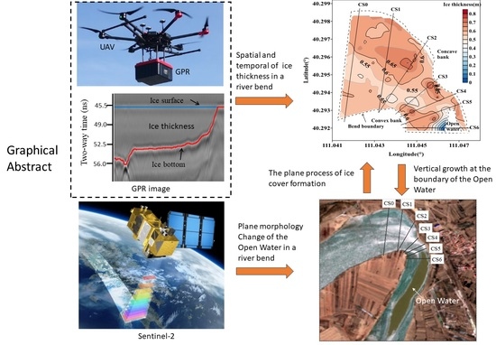
Morphology Dynamics of Ice Cover in a River Bend Revealed by the UAV-GPR and Sentinel-2

Abstract

After the formation of the bend ice cover, the ice thickness of the bend is not uniformly distributed, and an open-water area is usually formed downstream of the bend. The spatial and temporal variation of the ice thickness in seven cross sections was determined via Unmanned Aerial Vehicle Ground Penetrating Radar (UAV-GPR) technology and traditional borehole measurements. The plane morphology change of the open water was observed by Sentinel-2. The results show that the average dielectric permittivity of GPR was 3.231, 3.249, and 3.317 on three surveys (5 January 2022, 16 February 2022, and 25 February 2022) of the Yellow River ice growing period, respectively. The average ice thickness of the three surveys was 0.402 m, 0.509 m, and 0.633 m, respectively. The ice thickness of the concave bank was larger than that of the convex bank. The plane morphology of the open water first shrinks rapidly longitudinally and then shrinks slowly transversely. The vertical boundary of the open water was composed of two arcs, in which the slope of Arc I (close to the water surface) was steeper than that of Arc II, and the hazardous distance of the open-water boundary was 10.3 m. The increased flow mostly affected the slope change of Arc I. Finally, we discuss the variation of hummocky ice and flat ice in GPR images and the physical factors affecting GPR detection accuracy, as well as the ice-thickness variation of concave and convex banks in relation to channel curvature.

1. Introduction

The formation and development of river ice is a complex process that is affected by meteorological, hydrological, and topographical conditions [1,2]. Due to the particularity of the bend terrain, ice floes and frazil ice are easy to accumulate and form juxtaposed ice covers, which greatly reduce ice transport capacity [3] and, in severe cases, raises water levels, causing ice disasters. The accumulation area of the bend is hummocky ice, and the other area is flat ice. At the same time, open water is usually formed downstream of the bend due to the reduction in ice floes and increase in the hydraulic slope [4]. Due to the combined effect of low air temperature (less than 0 °C) and turbulent water flow, the existence of open water will cause an increase in frazil ice, which will block the downstream river and form ice jams in serious cases. Monitoring changes in the ice thickness and open water in the bend is important for modern society in many respects, for example, in relation to simulation of ice cover in the bend [5], analyses of ice-induced scour and erosion in ice engineering [6], and ice flood forecasting [7,8,9].

Ice thickness, one of the most important physical parameters of river ice, and its distribution, directly determine the process of ice growth and thawing at the bend with the combined action of meteorology and hydrodynamics. The traditional monitoring method is to drill holes, which has high credibility but low efficiency and high working intensity. Other high precision methods for measuring ice thickness have since been developed, e.g., thermal resistance wires [10] and ultrasonic waves [11,12], but they cannot adapt to the spatial survey of ice thickness because they need to be fixed on the ice sheet.

Ground penetrating radar (GPR) is a very useful nondestructive detection technology for mapping ice thickness [13]. Ice thickness can be calculated by obtaining the round-trip time of electromagnetic waves in the ice sheet and the corresponding radar speed or dielectric permittivity. GPR has been used extensively in sea ice [14,15,16], glacier ice [17,18], and river/lake ice [19,20,21,22], and is also deployed in manual towing, surface vehicles, aircrafts, and satellites [23]. In the late 1980s, some ice-thickness profiles of the Tanana River and Yukon River in Alaska were obtained by helicopter-mounted short-pulse radar with 500 MHz, 600 MHz, and 900 MHz antennae, respectively [24,25,26]. Li et al. [27] detected ice thickness at 25 points and analysed theoretically the influence of gas bubble content and ice crystal structures on dielectric permittivity. Liu et al. [28] tested the ice thickness of two 50 m long lines using the GPR system they developed. Kämäri et al. [29] surveyed the ice thickness of 45 cross-sections with high-frequency GPR of 800 MHz in a meandering shallow river. Fu et al. [30,31] developed double-frequency GPR to measure ice thickness and water depth simultaneously and presented a recommended range of values for the dielectric permittivity. Bai et al. [32] developed a layer-tracking method for ice-thickness detection based on GPR mounted on a UAV. Deng et al. [33], Wei et al. [34], and Li et al. [13] measured ice thickness automatically and continuously at a fixed position by hanging GPR throughout the ice period. These previous studies focused on testing GPR technology or analyzing dielectric permittivity. However, this paper mainly presents the detailed morphology changes of the ice cover of a river bend using GPR technology, which is useful to understand the characteristics and the mechanism of ice-cover formation and reduce ice disasters.

Remote sensing technology is another approach for providing river ice information, but the spatial resolution of images needs to be able to distinguish between ice, water, and the surrounding landscape [35]. High-resolution images from satellites such as Sentinel-2A/B (10 m) and Landsat (30 m) could be used to measure the length and area of river ice, to classify river ice, open water, and land [36,37], to reveal temporal and spatial distribution characteristics [38], to extract river ice phenology [39], and to identify ice jams and ice dams [40]. Moreover, moderate resolution (0.25–1 km) and high temporal resolution images such as moderate-resolution imaging spectroradiometer (MODIS) and advanced very high-resolution radiometer (AVHRR) are often used to study ice breakups in near-infrared bands [35]. Synthetic aperture radar (SAR) images, insensitive to cloud cover, are commonly used to identify ice surface roughness and classification [41] and to retrieve ice thickness [42,43]. However, to our knowledge, previous studies have not studied the evolution of open water formed after ice cover in the bend by remote sensing, which helps refine computer simulations of open water changes in the future.

This paper provides unique information on spatial and temporal variations of river ice thickness and open water in the Shisifenzi bend of the Yellow River using UAV-GPR and Sentinel-2. The aims were (1) to analyze the spatial and temporal characteristics of river ice thickness in the Shisifenzi bend, (2) to analyze the change characteristics of open water downstream of the bend, (3) to quantify the river flow’s influence on the ice growth at the open-water boundary, and (4) to discuss the factors affecting the accuracy of using UAV-GPR to detect hummocky ice and flat ice in the Shisifenzi bend and the change features of the ice thickness in the concave and convex banks.

2. Materials and Methods

2.1. Study Area

The study area (Figure 1) is in Inner Mongolia, China, which is a semi-arid region, with dry winters and little snow. Figure 2a shows the Shisifenzi bend (111°2′53″E, 40°17′39″N) in the mainstream of the Yellow River, which is a typical funnel bend characterized by a wide entrance and a narrow exit. The angle of the bend is about 120°, the hydraulic slope is about 0.1%, the average altitude is 991.8 m, the river width is 250–600 m, and the average water depth is 8 m. The Toudaoguai hydrological station is 3.1 km away from this bend, which recorded a stream flow of 325–1190 m³/s during the ice period of 2021–2022. The concave bank revetment is made of erosion protection measures in the form of galvanized iron wire gabions. The convex bank is a wasteland and has no protection.

According to records of the video camera system [13,33] fixed at the bend, sporadic ice floes appeared on the concave bank at 00:00 on 20 November 2021, with an air temperature of −8 °C. Afterward, the ice floes increased gradually, and ice concentration increased accordingly. At 7:00 on 18 December 2021, ice cover first formed at the narrow location of the bend, i.e., between sections CS3 and CS5 in Figure 2a. Meanwhile, many ice floes accumulated upstream, and the open water was formed downstream of the bend. On 28 February 2022, the ice cover began to melt and thin. At 14:00 on 13 March 2022, the ice cover of the bend cracked and slid downstream, and the ice cover completely disappeared at 16:00 on 15 March 2022.

2.2. Ice Thickness Measurement Using UAV-GPR

Figure 2b shows that the UAV-GPR, named IGPR-30, is equipped with a DJI M600, an air-coupled GPR with a central frequency of 400 MHz, the Trimble Real-Time Kinetic Global Positioning System (RTK GPS), and a two-megapixel infrared camera. The GPR weighs approximately 3.5 kg and is designed to detect ice thickness of 6 m, with a sampling frequency of 5 GHz and ice-thickness resolution of 1 mm. The fully loaded UAV is remotely controlled with a range of 2 km and can fly continuously for 15–30 min at −30 °C.

Figure 2c shows how the ice-thickness detection system works, with the transmitting antenna emitting electromagnetic waves into the ice cover and the receiving antenna collecting the reflected waves from the air–ice interface and the ice–water interface, respectively. The ice thickness is detected at average intervals of 1 m on the flight path, with the RTK GPS giving the coordinates of each measurement point. The infrared camera records the ice surface conditions in real time.

Three surveys with the UAV-GPR were carried out at the Shisifenzi bend during the ice growth period of winter 2021–2022, on 5 January 2022 (green solid line in Figure 2a), 16 February 2022 (red solid line in Figure 2a), and 25 February 2022 (blue solid line in Figure 2a). The flight on 5 January 2022 was near the CS3 section and was mainly to test the performance of the UAV-GPR system, which is why it differed from the flight paths on February 16 and 25. The UAV flew from the concave bank to the convex bank in a single flight and then returned to the concave bank. To ensure the stability of radar detection, the flight speed was generally controlled at 2–3 m/s, and the single flight time was approximately 5–8 min. The height of the UAV-GPR from the ice surface was controlled in the range of 5–10 m to reduce the attenuation of electromagnetic waves in the air, and the GPR detection time window was set to 70 ns. Seven cross sections (black dash line in Figure 2a) were planned, named CS0, CS1, CS2, CS3, CS4, CS5, and CS6 from upstream to downstream, respectively. These cross sections were as close as possible to the UAV flight paths.

Due to the large number of obstacles e.g., trees and telegraph poles on both banks, we did not use the automatic flight function but used the manual flight control to detect the ice thickness. In the upstream of the bend, some flight paths did not reach the convex bank since the sight distance was longer. Some ice thickness was not detected due to the sudden increase in flight height resulting in exceeding the detection time window, especially upstream of CS0. Finally, we obtained 1124 valid radar ice thickness data on 5 January 2022, 4043 valid ice thickness data on 16 February 2022, and 3449 valid radar ice thickness data on 25 February 2022.

Figure 3 shows the typical GPR profile obtained on 25 February 2022. The stepped GPR image (dotted box) of the concave bank is the gabions revetment. The layer tracking algorithm [32] supplemented by manual corrections was used to track the air interface, ice–air interface, and ice–water interface in the GPR profile. The ice thickness was calculated by Equations (1) and (2).

$$H_i=v_i∆t/2=v_i\left(t_1-t_2\right)/2,$$

(1)

$$v_i=\mathrm{c}/\sqrt{{\epsilon }_i},$$

(2)

where $H_i$ is the ice thickness detected by IGPR-30, cm; $v_i$ is the radar wave velocity in the ice cover, cm ns⁻¹; $∆t$ is the two-way time in the ice cover, ns; $t_1$ and $t_2$ are the two-way time from radar-air interface to ice-water interface and to ice-air interface, respectively, ns; and $c$ is the propagation velocity of the radar wave in air, equal to 30 cm ns⁻¹; ${\epsilon }_i$ is the dielectric permittivity of ice.

2.3. Open Water Monitoring with Sentinel-2

Sentinel-2 has two satellites (2A and 2B), with a Multi-Spectral Imager (MSI) covering 13 spectral bands and an image width of 290 km. The L2A-level images, processed with geometric correction, radiometric calibration, and atmospheric correction, were downloaded for free at the Copernicus Open Access Hub (https://scihub.copernicus.eu/dhus/#/home (24 November 2021, 4 December 2021, 19 December 2021, 24 December 2021, and 29 December 2021, 13 January 2022, 2 February 2022, 22 February 2022, 4 March 2022, and 14 March 2022)). The RGB true color images of Band 2, Band 3, and Band 4 combination were selected with a spatial resolution of 10 m.

In order to study the change characteristics of the open water in the winter of 2021–2022, eight images with less clouds were selected, corresponding to 19 December 2021, 24 December 2021, 29 December 2021, 13 January 2022, 2 February 2022, 22 February 2022, 4 March 2022, and 14 March 2022. Based on the ESRI’s ArcMap software, the boundaries of the open water were delineated manually, and data such as length, width, and area were also calculated.

In order to analyze the accumulation of floating ice in the early freeze-up, three images on 24 November 2021, 4 December 2021, and 9 December 2021 were selected.

2.4. Measured Ice Thickness and Dielectric Permittivity

Nature ice cover is the composite of pure ice and other substances. Air bubbles, unfrozen water, and sediment are the main factors affecting the dielectric permittivity of the ice cover. The dielectric permittivity of air bubbles, pure ice, unfrozen water, and sediment are 1, 3.17, 81, and 5.5, respectively [13].

In order to obtain the dielectric permittivity of the ice cover during the different periods, ice thickness ($H_i$) was measured by a Kovacs ice drill with 0.09 m diameter and ice-thickness measuring gauges (Roseburg, OR, USA). We drilled 2, 19, and 8 ice holes on 5 January 2022, 16 February 2022, and 25 February 2022, respectively. The 29 ice holes overlapped with the UAV flight paths, and the two-way time ($t_1-t_2)$ of the ice cover in the radar image of the corresponding location was obtained. The dielectric permittivity (${\epsilon }_i$) was calculated based on Equations (1) and (2).

Table 1. The dielectric permittivity on the three surveys.

Time	Measured Ice Thickness (cm)	Two-Way Time (ns)	Dielectric Permittivity	Average Dielectric Permittivity for Each Survey
5 January 2022	50.5	6.089	3.271	3.231
	54.6	6.501	3.190
16 February 2022	57.0	6.387	2.825	3.249
	66.0	6.638	2.276
	81.4	8.827	2.646
	68.7	10.720	5.478 *
	66.8	9.820	4.862 *
	83.8	7.846	1.973 *
	84.4	10.025	3.174
	82.8	9.717	3.099
	70.6	9.307	3.910
	75.6	8.828	3.068
	56.8	7.391	3.809
	62.6	7.493	3.224
	69.0	8.162	3.148
	63.0	7.504	3.192
	83.8	9.956	3.176
	87.0	11.061	3.637
	94.6	11.251	3.182
	92.2	11.529	3.518
	64.8	8.746	4.098
25 February 2022	65.1	7.769	3.205	3.317
	61.8	7.436	3.258
	63.7	7.671	3.263
	55.8	6.848	3.389
	67.8	8.184	3.278
	87.9	10.600	3.272
	84.9	10.621	3.521
	78.6	9.587	3.347

* The outlier values, which are not included in the calculation of the average dielectric permittivity. The reasons for the appearance of outlier values are discussed in Section 4.1.

shows the calculated dielectric permittivity for the three surveys. The average dielectric permittivity of each survey was 3.231, 3.249, and 3.317 on 5 January 2022, 16 February 2022, and 25 February 2022, respectively. Since there was sediment within the Yellow River ice, three average values were larger than the pure ice dielectric permittivity of 3.17 [13]. This paper calculated the valid ice thickness data using the average dielectric permittivity for the corresponding survey time. Figure 4 shows the ice thickness measured by ice drill compared with the ice thickness measured by GPR.

2.5. Spatial Interpolation Processing

In order to analyze the spatial and temporal distribution characteristics of the ice thickness of the bend, the detected ice thickness data were interpolated onto the 10 m-by-10 m grid using the natural neighborhood method of the Surfer software. The overlapping area of the interpolation results between 16 February 2022 and 25 February 2022 was selected for the study area. The boundaries of the bend and open water were delineated manually using ESRI’s ArcMap software based on the orthophoto image taken by DJI Phantom 4 on 27 February 2022. The interpolated data outside the boundary of the bend and open water were removed based on the boundary files (SHP format) using the Surfer’s blank method. In addition, the interpolated result on 5 January 2022 was removed only for data outside the bend boundary. After interpolation to generate ice-thickness contour maps, we also plotted the profile along CS0, CS1, CS2, CS3, CS4, CS5, and CS6 in the Surfer software, respectively.

3. Results

3.1. Spatial and Temporal Distribution of Ice thickness

Figure 5a is the contour map of the ice thickness near CS3 (narrowest part of the bend) on 5 January 2022. The spatial distribution of the ice thickness was not uniform, and the ice thickness of the concave bank was larger than that of the convex bank. The average ice thickness was 0.402 m with a standard deviation of 0.044 m. In the region, the minimum ice thickness of 0.259 m was in the middle of CS3. This is because this is the location of the main channel where larger flow velocity under the ice cover can inhibit ice growth, which is consistent with the observation of Kämäri et al. [29]. However, the maximum ice thickness of 0.555 m was in the concave bank. This is because in the early stages of ice-cover formation, a large amount of ice floes and frazil slush flowed towards the concave bank (CS3) and formed greater initial ice thickness in the concave bank. In addition, this survey (5 January 2022) was less than a month after the ice cover formed (18 December 2021). Frazil ice upstream may have continued to flow toward the concave bank of CS3 and accumulated under the ice cover.

Figure 5b,c show that the ice-thickness distribution in the bend was uneven on 16 February 2022 and 25 February 2022. The ice thickness characteristic values are shown in

Table 2. The characteristic values of the ice thickness distribution in the bend for the three surveys.

Time	Ice Thickness (m)
	Minimum Value	Maximum Value	Average Value	Standard Deviation
5 January 2022	0.259	0.555	0.402	0.044
16 February 2022	0.004	0.781	0.590	0.066
25 February 2022	0.007	0.964	0.633	0.082

. In Figure 5b,c, the thin ice strip, connected to open water, could be clearly observed. The previous observation of flow velocity under ice cover showed that this strip area was the main channel with a large flow velocity [44]. Li et al. [45] built the improved Stefan equation with additional flow velocity based on data from the Songhuajiang River, northeast of China, which showed that the higher the flow velocity the lower the ice thickness. Moreover, the ice thickness and flow velocity in the Sävar River, in the northern part of Sweden, observed by Polvi et al. [46], showed that ice thickness is thinner in areas of large flow velocity.

In addition, the ice thickness was thicker near the concave bank in the upstream of CS3. On 16 February 2022, the average ice thickness of the concave bank for CS0, CS1, CS2, and CS3 were 0.539 m, 0.624 m, 0.634 m, and 0.614 m, respectively. The average ice thickness of the convex bank for CS0, CS1, CS2, and CS3 were 0.569 m, 0.547 m, 0.523 m, and 0.543 m, respectively. On 25 February 2022, the average ice thickness of the concave bank for CS0, CS1, CS2, and CS3 were 0.586 m, 0.678 m, 0.755 m, and 0.648 m, respectively. The average ice thickness of the convex bank for CS0, CS1, CS2, and CS3 were 0.574 m, 0.589 m, 0.645 m, and 0.565 m, respectively.

Two peak areas are observed in the concave bank of Figure 5b, and the obvious groove was formed between CS2 and CS3. In Figure 5c, the two peak areas can also be observed in the concave bank, but the groove is less obvious, and the ice-thickness contour tends to smooth out. The ice thickness in the groove grew a little faster. It seems more likely that the reduced flow velocities in the groove allowed for greater thermal ice growth from 16 February 2022 to 25 February 2022, since ice thickness is thicker where the flow velocity is low [45,46].

Figure 5d is the contour map of ice-thickness growth in the bend from 16 February 2022 to 25 February 2022. It shows that the mainstream area ice thickness grew less; meanwhile, the non-mainstream area grew more. This may be due to the large flow velocity in the mainstream inhibiting the ice-thickness growth. In the region between CS0 and CS5, the average growth rate of the ice thickness in the mainstream region was 0.006 m d⁻¹ with a standard deviation of 0.003 m d⁻¹, and the average growth rate of ice thickness in the non-mainstream region was 0.008 m d⁻¹ with a standard deviation of 0.005 m d⁻¹. The growth rate of ice thickness in the non-mainstream region was 1.242 times faster than that in the mainstream from 16 February 2022 to 25 February 2022.

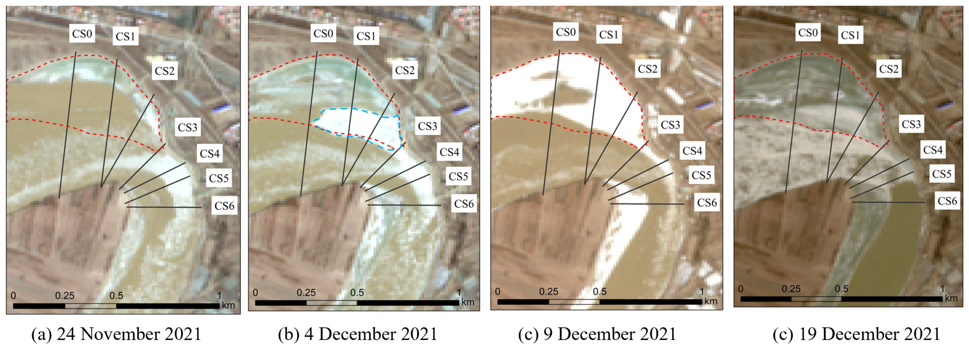
3.2. Plane Morphology Change of the Open Water

The high-resolution Sentinel-2 images were used to observe the plane changes of the open water throughout the winter of 2021–2022. Figure 6 shows the process from the formation (Figure 6a) to the disappearance (Figure 6h) of the open water in the Shisifenzi bend. The open water was diamond-shaped, narrow upstream and downstream and wide in the middle. Moreover, as the ice cover grew, the area of the open water was reduced. The area reduction was divided into two stages, rapid reduction (Figure 6a–c) and slow reduction (Figure 6c–g).

In order to quantitatively describe the change of the open water, the ESRI’s ArcMap platform was used to measure the length, width, and area of the open water. Both CS7 and CS8 were used to observe the transversal changes of the open water, and their cross-section lengths were 292.5 m and 360.7 m, respectively. The longitudinal length of the initial formed open water (Figure 6a) was 2886.7 m, and the total area of the channel downstream of the bend shown in Figure 6a was 970,543 m². The subsequent changes in the length, width, and area of the open water were normalized. The relative length is the open water actual length divided by the total length (2886.7 m) of the initial formed open water. The relative width is the open water actual length divided by the channel width. The relative area is the open water actual area divided by the total area (970,543 m²) of the channel downstream of the bend. The results are shown in Figure 7a.

In Figure 7a, the relative area rapidly shrank from 0.59 to 0.17 in the first stage. During this phase (from 19 December 2021 to 29 December 2021), average air temperature dropped extremely from −3.0 °C to −16.4 °C, as shown in Figure 7b. More frazil ice quickly accumulated downstream of the open water, causing rapid reduction. In the second stage, the relative area slowly shrank from 0.17 to 0.13. During this phase (from 29 December 2021 to 4 March 2022), the average air temperature rose, then fell, then rose again, and each process was slow, as shown in Figure 7b. Due to the lack of lower negative air temperature, the ice cover near the open water grew slowly transversely, so the open-water area was also reduced slowly. Moreover, the change in the relative longitudinal length was similar to the change in the relative area, which rapidly decreased from 1 to 0.48 in the first stage but remained almost constant at 0.46 in the second stage.

In addition, for CS7 in the upper part of the open water in Figure 7a, the relative width was reduced from 0.65 to 0.55 in the first stage and then to 0.41 in the second stage. The new growth of ice cover in the open water was mainly located on the right bank, and there was no change on the left bank since the left bank is a mainstream region with a high flow velocity. The transverse growth rate of the ice cover on the right bank slowed down with time, since there was no lower and longer negative air temperature to promote ice-cover growth. During this stage, the average air temperature was on an upward trend, up to −2.5 °C on 22 January 2022, as shown in Figure 7b. For CS8 in the lower part of the open water in Figure 7, the open water width was quickly reduced from 0.74 to 0.24 in the first stage due to the accumulation of the broken bank ice and frazil ice driven hydrodynamically. Afterward, it remained almost constant at 0.23 in the second stage. This was because the hydrodynamic erosion capacity was equal to the thermal growth capacity of ice cover when the open water was narrowed to a certain extent. In the future, an unmanned boat carrying Acoustic Doppler Current Profilers (ADCP) could be used to measure the three-dimensional velocity in the open water at a different period to quantify the relationship between hydrodynamic erosion and thermal growth of the ice cover in open water.

3.3. Vertical Growth of Ice Thickness at the Boundary of the Open Water

When the UAV-GPR flew over the open water, the open-water area was shown as a straight line in the radar image and the ice thickness at the open-water boundary can be clearly distinguished. This way could detect the vertical growth of the ice cover at the boundary of the open water, which was the supplement of the remote sensing plane observation. Since the UAV route was not perpendicular to the open-water boundary, the original radar ice thickness was projected vertically along the open-water boundary. The projected ice thickness at the boundary of the open water is shown in Figure 8 (results of the 16 February 2022) and Figure 9 (results of the 25 February 2022). Figure 8a–c and Figure 9a–b represent the ice thickness at the boundary of the open water on the convex bank. Figure 8d–f and Figure 9c–d represent the ice thickness at the boundary of the open water on the concave bank.

Figure 8 and Figure 9 show that the ice cover at the boundary was of two arcs, named Arc I and Arc II, respectively. Arc I was close to the open-water surface and was relatively steep. Its ice cover was thin and had a low bearing capacity, which was the most dangerous area. However, Arc II had a gentle slope. Its ice cover thickened and the bearing capacity increased.

The starting ice thickness of Arc II on 16 February 2022 was between 0.34 m and 0.51 m, with an average value of 0.43 m; the starting ice thickness of Arc II on 25 February 2022 ranged from 0.41 m to 0.53 m, with an average value of 0.45 m.

Considering the safety of working on ice covers, the horizontal distance of Arc I was defined as the hazardous distance of the boundary of the open water. The hazardous distance on 16 February 2022 was between 3.47 m and 7.28 m; the hazardous distance on 25 February 2022 ranged from 6.63 m to 10.3 m. The most hazardous distance was 10.3 m near the open water.

In order to analyze the characteristics of the ice cover vertical growth, the average slope, i.e., ice thickness divided by the horizontal distance, of Arc I and Arc II were calculated, respectively. The slope at different locations and different times of the open water was plotted with the inlet of the open water as the distance 0 point, as shown in Figure 10.

Figure 10a shows that the slope of Arc I on 25 February 2022 (5.79%) was smaller than the slope on 16 February 2022 (8.10%), which meant that the slope of Arc I on 25 February 2022 was gentler and the vertical growth of the ice cover was slower. This was caused by an increased discharge which broke the original balance of hydrodynamic erosion and the thermal growth of the ice cover. Figure 10c shows the flow increased from 583 m³/s to 654 m³/s between 16 February 2022 and 25 February 2022. In addition, we found that the further away from the inlet of the open water, the smaller the slope of Arc I. The slope of Arc I of the convex bank was generally larger than that of the convex bank. That is to say, the convex bank slope was steeper, which was because the bend flow scoured the ice cover on the concave bank and the hydrodynamics inhibited the vertical growth of the concave bank ice. The average slope of the convex and concave banks for two measurements were 8.60% and 6.10%, respectively. If the slope change of Arc I was used to express the hydrodynamic inhibition ability of the growth of the concave bank ice cover, the hydrodynamic inhibition of the concave bank was 30% greater than that of the convex bank in the ice growth of the open water.

Figure 10b shows that the slope of most of Arc II was significantly smaller than that of Arc I. There was no obvious change in the slope of the concave and convex banks and no effect of the slope slowing produced by the continuous increase in the river flow. These indicate that the flow in the open water mainly affected the ice-cover growth in Arc I.

4. Discussion

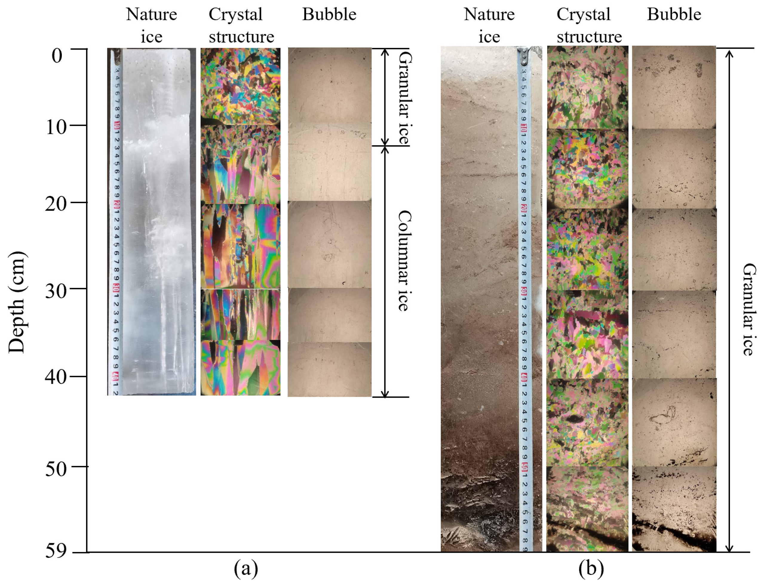
4.1. Detection of Hummocky Ice and Flat Ice Using UAV-GPR

When ice freezes up in the bend, ice floes in the mainstream squeeze and stack on each other, forming hummocky ice (HI) with larger ice surface roughness (Figure 11a). The ice floes in the non-mainstream freeze steadily, forming flat ice (FI) with small ice surface roughness (Figure 11b). In general, the material composition of HI is more complex than that of FI. During radar detection of the ice thickness, the radar waves will be strongly reflected when they encounter materials with different dielectric permittivity. The greater the difference in dielectric permittivity, the stronger the reflected wave.

Figure 12a shows the radar image of part of CS3 at the beginning of the ice cover (5 January 2022). In the HI area, the amplitude of the radar reflections from the ice surface and ice bottom are strong, showing irregular pleat shapes. It is not easy to automatically track the interfaces of air–ice and ice–water using layer-tracking algorithms [32]. Manual tracking interfaces and interpretation are required. The reason for the HI radar image is that the interfaces of air–ice and ice–water are uneven with large gaps, as shown in Figure 12a. The radar waves may repeatedly encounter air–ice–air…ice on the ice surface, and ice–water–ice…water on the ice bottom, forming a cluttered interface. In the FI area, the air–ice interface can be clearly distinguished automatically due to the flatted ice surface. A small pit, shown in the red dotted box in Figure 12a, appears on the ice-water in the FI area, which may be caused by water scouring.

Figure 12b,c give the radar image of part of CS3 at the end of the ice-cover growth (16 February 2022 and 25 February 2022). Compared with the HI image on 5 January 2022, shown in Figure 12a, the air–ice interface becomes smooth and can be tracked automatically. The combined effects of diurnal air temperature difference, solar radiation, and wind make the surface of the HI melt and become relatively flat. Sometimes, the small amount of snowfall will fill the surface gaps in the HI area. In addition, the ice–water interface of the HI area becomes a regular hyperbolic shape, which can also be clearly distinguished. This may be due to water scouring, which makes small irregular gaps into large regular gullies in the ice bottom.

The accuracy of measuring HI and FI using UAV-GPR is different. The measurement error of FI is basically within 10%, and the error of HI is about 10%-15% based on the 54 measured ice thickness data in the Yellow River ice [47]. We consider two reasons for the large error of HI from a measurement aspect. (1) The ice surface or ice bottom in the HI area may be uneven, which means we could not obtain the accurate measured ice thickness when drilling. (2) Two-way time of drilling location could not be obtained accurately due to the irregular interface in the radar image of a cross-section, especially at the early stage of freezing. Sometimes, some unreasonable dielectric permittivity, e.g., 5.478, 4.862, and 1.973 in Table 1, would be calculated by Equations (1) and (2). This is because the continuous GPR image resolution is small for the single borehole location, leading to an unreasonable two-way time acquisition, especial in the HI area. In the future, when UAV-GPR flies above the drilling position, it should stay for a few seconds to obtain a stable two-way time.

The dielectric permittivity or radar wave velocity is the central factor in the accuracy of radar detection of ice thickness. For ice physics, Yellow River natural ice is a four-phase mixture of pure ice, bubbles, sediment, and unfrozen water. The dielectric permittivity of natural ice should be the combination of a four-material dielectric permittivity based on volume ratio. Two ice samples (Figure 13) were cut on 14 February 2022 in the areas of HI and FI, respectively. The ice thickness of the HI was thicker than that of the FI. FI in Figure 14a has a small amount of sediment and air bubbles on the surface layer, while the rest of the ice is shining brightly. Its surface layer 0–13 cm is granular ice and 13–42 cm is columnar ice. For HI in Figure 14b, the sediment content in ice gradually increases and the bubble content is more and unevenly distributed. The crystal type of HI is granular from 0 cm to 59 cm. In addition, the air bubble and sediment content and distribution within the ice are random, and the unfrozen water content will change in phase with ice temperature and grain boundary size. Therefore, it is a challenge to accurately detect the ice thickness using GPR.

Previous field experiments have found that the radar wave velocity was larger during the ice growth period than during the ice melting period. It might be influenced by the air temperature [48]. Li et al. [13] revealed that the unfrozen water content in the ice was the central factor controlling the variation of radar wave velocity. The unfrozen water content depended on the ice temperature, which in turn was controlled by air temperature, solar radiation, and ice thickness. Based on such a physical mechanism, two radar wave velocity correction models (Logistic Function) were constructed based on the air temperature (Equation (3)) or the combination of air temperature and the previous time of ice thickness (Equation (4)), respectively.

$$v_r=A/(1+C_1{e}^{D_1{\theta }_a})+B,$$

(3)

$$v_r=A/(1+\left(C_1+C_{2}h+C_3{h}^2+C_4{h}^3\right)e^{\left(D_1+D_{2}h+D_3{h}^2+D_4{h}^3\right){\theta }_a})+B,$$

(4)

where, $v_r$ represents the radar wave velocity; ${\theta }_a$ represents the air temperature; $h$ represents the previous ice thickness; the sum of $A$ and $B$ indicates the radar wave velocity of three-phase Yellow River ice; $B$ indicates the radar wave velocity of two-phase Yellow River water, with A and $B$ obtained by statistical optimization under theoretical guidance; and $C_1,C_2,C_3,C_4,$ $D_1,D_2,D_3,$ and $D_4$ represent the accommodation coefficient and logistic growth rate, respectively. Their values are chosen in

Table 3. Correlation coefficient in Equation (3).

Coefficients	Air Temperature
	Rising Process		Falling Process
	Granular Ice	Columnar Ice	Granular Ice	Columnar Ice
A	13.6800	13.6800	13.6800	13.6800
B	3.3300	3.3300	3.3300	3.3300
C1	0.033	0.032	0.061	0.060
D1	0.163	0.165	0.147	0.148

of [13].

Since there was no previous time of ice thickness at the same position of the UAV measurements, we used the correction model based on air temperature (Equation (3)) to correct the radar wave velocity in the areas of the HI and the FI. The air temperature needed for calibration was sourced from the Toudaoguai hydrological station which is 3.1 km from the Shisifenzi bend. Depending on whether air temperature was rising or falling at the time of the measured ice thickness, the corresponding coefficient was chosen in Table 3. The correlation coefficient for the 0–13 cm ice layer was chosen for granular ice in Table 3. The remaining ice layer was chosen for columnar ice in Table 3. Finally, the corrected ice thickness at the location of the ice hole was calculated by weighing the thickness of the granular ice and the columnar ice.

The corrected results show that the correction effect of the FI was better than that of the HI. After correction, the root mean square error (RMSE) of the radar wave velocity in the FI was reduced by 4.38%, but the RMSE of the radar wave velocity in the HI increased by 3.90%. This may be because the correction model of Li et al. [13] was constructed based on the data of the FI. The model did not consider the high sediment content in the HI. In the future, we should continue to explore the relationship between high sediment content in ice and radar wave velocity and develop new correction models.

Although there is some error in the ice-thickness measurement by the UAV-GPR, its efficiency is high. In general, it takes 1.5 h for two people to measure the ice thickness of seven cross sections in the Shisifenzi bend. In addition, in the emergency monitoring, i.e., ice floes, thin ice, ice jams, ice dams, and ice in the melting period, UAV-GPR could significantly improve the efficiency of ice-thickness measurement and ensure people’s safety.

4.2. Comparison of the Ice Thickness on Concave and Convex Banks

In order to quantify the ice thickness variation of the concave and convex bank in the bend, the ice thickness comparison parameter ($M$) was introduced. The calculation formula is shown in Equation (5). The $M$ values of CS0–CS6 sections were calculated, respectively. The positive values of $M$ indicate the ice thickness of the concave bank was thicker than that of the convex bank, while negative values were the opposite.

$$M=\left(H_{ca}-H_{cv}\right)/H_{cv},$$

(5)

where $M$ is the percent; $H_{ca}$ is the average ice thickness of the concave bank, m; and $H_{cv}$ is the average ice thickness of the convex bank, m. The location of the thalweg was used to divide the concave bank and convex bank.

Figure 14a shows the average ice thickness and standard deviation of the concave and convex banks for three surveys from CS0 to CS6. Using CS3 as the river midline distance point 0, the upstream section was positive and the downstream section was negative. The ice thickness was thicker near the concave bank in the upstream of CS3 in the three surveys. As shown in the red dotted area of Figure 15, there was a very large and relatively calm flow area in the concave bank upstream of CS3. Early in freeze-up, more ice floes and frazil slush upstream accumulated in the area, which formed a greater initial ice thickness in the concave bank. Moreover, the area may likely have greater thermal ice-cover growth in the winter since it is far from the thalweg.

Figure 14b shows that the M of the three surveys in CS3 were not significantly different, which were 13.8%, 12.9%, 14.7% on 5 January 2022, 16 February 2022, and 25 February 2022, respectively. In the upstream of CS3, the M value gradually increased from CS0 to CS2 on 16 February 2022 and 25 February 2022. The maximum M was 21.2% in CS2. This may be the result of early ice-cover formation. As shown in the blue dotted area of Figure 15b, the big accumulation area formed and CS2 is located at ahead of the accumulation body. The ice thickness in the concave bank of CS2 may be thicker.

In the downstream of CS3, the M values on 16 February 2022 were negative, indicating that the ice thickness was thicker near the convex bank. This may be the result of larger initial ice thickness in the early freeze-up since the convex bank in the downstream of CS3 is the slow flow area where ice floes are easily captured. Meanwhile, during the ice-cover growth period, high flow velocity in the concave bank inhibits the thermodynamic growth of ice cover. However, for CS4 and CS5 on 25 February 2022, the M values were positive, showing that the ice thickness was thicker near the concave bank. This means that the ice thickness of the concave bank grew faster than that of convex bank from 16 February 2022 to 25 February 2022, which exceeds the natural thermal growth rate of the ice cover. Figure 16 shows the discharge increased from 583 m³/s to 654 m³/s and the water level rose from 988.03 m to 988.17 m from 16 February 2022 to 25 February 2022. The increased discharge and water level may lead to the redistribution of unstable and unfrozen ice at the bottom of the ice, resulting in the local rapid increase in ice thickness near CS4 and CS5.

The change of M value is more likely to be related to the channel curvature. When the curvature becomes larger, the concave bank may more easily accumulate frazil slush and form the bigger initial ice thickness. In straighter reaches, the thalweg will be closer to the center of the channel and the flow conditions near the left and right banks will be more similar, and the M value would approach zero. In the future, we will look for bends with different curvatures to measure ice thickness using UAV-GPR and thus find their quantitative relationship. In addition, the flight path should coincide with the planned cross-section as much as possible.

5. Conclusions

Combined with UAV-GPR and Sentinel-2 technology, the process of river ice morphology change could be monitored. This paper studied the spatial and temporal variations of ice thickness and open water in the Shisifenzi bend of Yellow River. Some conclusions are listed as follows:

(1)

The average dielectric permittivity were 3.231, 3.249, and 3.317 on 5 January 2022, 16 February 2022, and 25 February 2022, respectively, which are larger than the pure ice dielectric permittivity of 3.17. The average ice thicknesses were 0.402 m ± 0.044 m, 0.509 m ± 0.066 m, and 0.633 m ± 0.082 m on the three surveys in the Shisifenzi bend, respectively.

(2)

The ice thickness distribution in the bend was uneven. The ice thickness was thicker near the concave bank in the upstream of CS3. In addition, the ice thickness was thinner in the mainstream. The average growth rate of ice thickness in the mainstream was 0.006 m d⁻¹, and in the non-mainstream region it was 0.008 m d⁻¹. The former was 1.242 times more than the latter.

(3)

In the downstream of the Shisifenzi bend, the plane morphology changes of the open water went through two stages. Firstly, the longitudinal length of the open water rapidly shortened, driven mainly by the hydrodynamic effect bringing frazil ice and broken bank ice. Secondly, the non-mainstream ice cover near the open water grew slowly transversely under the effect of accumulated negative air temperature.

(4)

The vertical growth of ice thickness at the boundary of the open water was not uniform. The ice-cover boundary was of two arcs, named Arc I (close to the open-water surface) and Arc II. The slope of Arc I was steeper than that of Arc II and the hazardous distance of the open-water boundary was 10.3 m. The increased flow made the change in the slope of Arc I, which broke the original balance of the hydrodynamic erosion and the thermal growth of ice cover. Moreover, it mostly affected the ice-cover growth change in Arc I, not in Arc II.

References

1. Shen, H.T. Mathematical modeling of river ice processes. Cold Reg. Sci. Technol. 2010, 62, 3–13. [Google Scholar] [CrossRef]
2. Beltaos, S.; Bonsal, B. Climate change impacts on Peace River ice thickness and implications to ice-jam flooding of Peace-Athabasca Delta, Canada. Cold Reg. Sci. Technol. 2021, 186, 103279. [Google Scholar] [CrossRef]
3. Chen, P.; Cheng, T.; Wang, J.; Cao, G. Accumulation and evolution of ice jams influenced by different ice discharge: An experimental analysis. Front. Earth Sci. 2023, 10, 1054040. [Google Scholar] [CrossRef]
4. Zhao, S.; Li, C.; Li, C.; Shi, X.; Zhao, S. Processes of river ice and ice-jam formation in Shisifenzi Bend of the Yellow River. J. Hydraul. Eng. 2017, 48, 351–358. (In Chinese) [Google Scholar] [CrossRef]
5. Zhai, B.; Liu, L.; Shen, H.T.; Ji, S. A numerical model for river ice dynamics based on discrete element method. J. Hydraul. Res. 2022, 60, 543–556. [Google Scholar] [CrossRef]
6. Smith, D.G.; Pearce, C.M. Ice jam-caused fluvial gullies and scour holes on northern river flood plains. Geomorphology 2002, 42, 85–95. [Google Scholar] [CrossRef]
7. Ferrick, M.G.; Mulherin, N. Framework for control of dynamic ice break-up by river regulation. Regul. River 1989, 3, 79–92. [Google Scholar] [CrossRef] [Green Version]
8. Mahabir, C.; Hicks, F.; Fayek, A.R. Neuro-fuzzy River ice breakup forecasting system. Cold Reg. Sci. Technol. 2006, 46, 100–112. [Google Scholar] [CrossRef]
9. Das, A.; Budhathoki, S.; Lindenschmidt, K. A stochastic modelling approach to forecast real-time ice jam flood severity along the transborder (New Brunswick/Maine) Saint John River of North America. Stoch. Environ. Res. Risk Assess. 2022, 36, 1903–1915. [Google Scholar] [CrossRef]
10. Lei, R.; Li, Z.; Qin, J.; Cheng, Y. Investigation of new technologies for in-situ ice thickness observation. Adv. Water Sci. 2009, 20, 287–292. [Google Scholar] [CrossRef]
11. Marko, J.R.; Jasek, M. Sonar detection and measurements of ice in a freezing river I: Methods and data characteristics. Cold Reg. Sci. Technol. 2010, 63, 121–134. [Google Scholar] [CrossRef]
12. Xie, F.; Lu, P.; Li, Z.; Wang, Q.; Zhang, H.; Zhang, Y. A floating remote observation system (FROS) for full seasonal lake ice evolution studies. Cold Reg. Sci. Technol. 2022, 199, 103557. [Google Scholar] [CrossRef]
13. Li, Z.; Li, C.; Yang, Y.; Zhang, B.; Deng, Y.; Li, G. Physical Mechanism and Parameterization for Correcting Radar Wave Velocity in Yellow River Ice with Air Temperature and Ice Thickness. Remote Sens. 2023, 15, 1121. [Google Scholar] [CrossRef]
14. Worby, A.P.; Griffin, P.W.; Lytle, V.I.; Massom, R. On the use of electromagnetic induction sounding to determine winter and spring sea ice thickness in the Antarctic. Cold Reg. Sci. Technol. 1999, 29, 49–58. [Google Scholar] [CrossRef]
15. Morozov, P.A.; Berkut, A.I.; Vorovsky, P.L.; Morozov, F.P.; Pisarev, S.V. Measuring Sea ice thickness with the LOZA geo radar. Russ. J. Earth Sci. 2021, 21, 3. [Google Scholar] [CrossRef]
16. Li, X.; Feng, X.; Liang, W.; Xue, C.; Zhou, H.; Wang, Y. A full-polarimetric GPR system and its application in ice crack detection. IOP Conf. Ser. Earth Environ. Sci. 2021, 660, 012026. [Google Scholar] [CrossRef]
17. Liu, J.; Wang, S.; He, Y.; Li, Y.; Wang, Y.; Wei, Y.; Che, Y. Estimation of Ice Thickness and the Features of Subglacial Media Detected by Ground Penetrating Radar at the Baishui River Glacier No. 1 in Mt. Yulong, China. Remote Sens. 2020, 12, 4105. [Google Scholar] [CrossRef]
18. Karušs, J.; Lamsters, K.; Ješkins, J.; Sobota, I.; Džeriņš, P. UAV and GPR Data Integration in Glacier Geometry Reconstruction: A Case Study from Irenebreen, Svalbard. Remote Sens. 2022, 14, 456. [Google Scholar] [CrossRef]
19. Best, H.; McNamara, J.P.; Liberty, L. Association of ice and river channel morphology determined using ground-penetrating radar in the kuparuk river, Alaska. Arct. Antarct. Alp. Res. 2005, 37, 157–162. [Google Scholar] [CrossRef] [Green Version]
20. Richards, E.; Stuefer, S.; Rangel, R.C.; Maio, C.; Belz, N.; Daanen, R. An evaluation of GPR monitoring methods on varying river ice conditions: A case study in Alaska. Cold Reg. Sci. Technol. 2023, 210, 103819. [Google Scholar] [CrossRef]
21. Han, H.; Li, Y.; Li, W.; Liu, X.; Wang, E.; Jiang, H. The influence of the internal properties of River Ice on Ground Penetrating Radar Propagation. Water 2023, 15, 889. [Google Scholar] [CrossRef]
22. Kovachis, N.; Maxwell, J.; Hicks, F. Suitability of aerial GPR deployments for river ice thickness mapping. In Proceedings of the 15th CRIPE Workshop on River Ice, St. John’s, NL, Canada, 15–17 June 2009. [Google Scholar]
23. Kemp, J.E.; Davies, E.G.R.; Loewen, M.R. Spatial variability of ice thickness on stormwater retention ponds. Cold Reg. Sci. Technol. 2019, 159, 106–122. [Google Scholar] [CrossRef]
24. Arcone, S.A.; Delaney, A.J. Airborne river-ice thickness profiling with helicopter-borne UHF short-pulse radar. J. Glaciol. 1987, 33, 330–340. [Google Scholar] [CrossRef] [Green Version]
25. Arcone, S.A. Dielectric permittivity and layer-thickness interpretation of helicopter-borne short-pulse radar waveforms reflected from wet and dry river-ice sheets. IEEE Geosci. Remote 1991, 29, 768–777. [Google Scholar] [CrossRef]
26. Delaney, A.J.; Arcone, S.A.; Chacho, E.F. Winter Short-Pulse Radar Studies on the Tanana River, Alaska. Arctic 1990, 43, 244–250. [Google Scholar] [CrossRef] [Green Version]
27. Li, Z.; Jia, Q.; Zhang, B.; Leppäranta, M.; Lu, P.; Huang, W. Influences of gas bubble and ice density on ice thickness measurement by GPR. Appl. Geophys. 2010, 7, 105–113. [Google Scholar] [CrossRef]
28. Liu, H.; Takahashi, K.; Sato, M. Measurement of dielectric permittivity and thickness of snow and ice on a Brackish Lagoon using GPR. IEEE J.-STARS. 2014, 7, 820–827. [Google Scholar] [CrossRef]
29. Kämäri, M.; Alho, P.; Colpaert, A.; Lotsari, E. Spatial variation of river-ice thickness in a meandering river. Cold Reg. Sci. Technol. 2017, 137, 17–29. [Google Scholar] [CrossRef]
30. Fu, H.; Liu, Z.; Guo, X.; Cui, H. Double-frequency ground penetrating radar for measurement of ice thickness and water depth in rivers and canals: Development, verification, and application. Cold Reg. Sci. Technol. 2018, 154, 85–94. [Google Scholar] [CrossRef]
31. Fu, H.; Guo, X.; Wang, T.; Xin, G.; Li, J.; Pan, J. Dielectric constant of ice in Natural Rivers. J. Hydrol. 2022, 615, 128700. [Google Scholar] [CrossRef]
32. Bai, X.; Wang, L.; Luo, X.; Mi, H.; Chen, H.; Liu, L.; Ji, M.; Gao, Y. A layer tracking method for ice thickness detection based on GPR mounted on the UAV. In Proceedings of the 4th International Conference on Imaging, Signal Processing and Communications (ICISPC), Kumamoto, Japan, 23–25 October 2020. [Google Scholar] [CrossRef]
33. Deng, Y.; Li, C.; Li, Z.; Zhang, B. Dynamic and full-time acquisition technology and method of ice data of Yellow River. Sensors 2021, 22, 176. [Google Scholar] [CrossRef] [PubMed]
34. Wei, Q.; Yao, X.; Zhang, H.; Duan, H.; Jin, H.; Chen, J.; Cao, J. Analysis of the variability and influencing factors of ice thickness during the ablation period in Qinghai Lake using the GPR ice monitoring system. Remote Sens. 2022, 14, 2437. [Google Scholar] [CrossRef]
35. Cooley, S.W.; Pavelsky, T.M. Spatial and temporal patterns in Arctic River ice breakup revealed by automated ice detection from MODIS imagery. Remote Sens. Environ. 2016, 175, 310–322. [Google Scholar] [CrossRef]
36. Zhang, X.; Jin, J.; Lan, Z.; Li, C.; Fan, M.; Wang, Y.; Yu, X.; Zhang, Y. ICENET: A Semantic Segmentation Deep Network for River Ice by Fusing Positional and Channel-Wise Attentive Features. Remote Sens. 2020, 12, 221. [Google Scholar] [CrossRef] [Green Version]
37. Zhang, X.; Yue, Y.; Han, L.; Li, F.; Yuan, X.; Fan, M.; Zhang, Y. River ice monitoring and change detection with multi-spectral and SAR images: Application over yellow river. Multimed. Tools Appl. 2021, 80, 28989–29004. [Google Scholar] [CrossRef]
38. Li, H.; Li, H.; Wang, J.; Hao, X. Monitoring high-altitude river ice distribution at the basin scale in the northeastern Tibetan Plateau from a Landsat time-series spanning 1999–2018. Remote Sens. Environ. 2020, 247, 111915. [Google Scholar] [CrossRef]
39. Li, H.; Li, H.; Wang, J.; Hao, X. Revealing the river ice phenology on the Tibetan Plateau using Sentinel-2 and Landsat 8 overlapping orbit imagery. J. Hydrol. 2023, 619, 129285. [Google Scholar] [CrossRef]
40. Zhang, F.; Mosaffa, M.; Chu, T.; Lindenschmidt, K.-E. Using remote sensing data to parameterize ice jam modeling for a northern inland delta. Water 2017, 9, 306. [Google Scholar] [CrossRef] [Green Version]
41. Palomaki, R.T.; Sproles, E.A. Quantifying the Effect of River Ice Surface Roughness on Sentinel-1 SAR Backscatter. Remote Sens. 2022, 14, 5644. [Google Scholar] [CrossRef]
42. Mermoz, S.; Allain, S.; Bernier, M.; Pottier, E.; Sanden, J.V.D.; Chokmani, K. Retrieval of river ice thickness from C-band PolSAR data. In Proceedings of the 2012 IEEE International Geoscience and Remote Sensing Symposium, Munich, Germany, 22–27 July 2012. [Google Scholar] [CrossRef] [Green Version]
43. Zhang, H.; Li, H.; Li, H. Monitoring the Ice Thickness in High-Order Rivers on the Tibetan Plateau with Dual-Polarized C-Band Synthetic Aperture Radar. Remote Sens. 2022, 14, 2591. [Google Scholar] [CrossRef]
44. Luo, H.; Ji, H.; Gao, G.; Zhang, B.; Mou, X. Study on the characteristics of flow and ice jam in Shisifenzi bend in the Yellow River during the freeze-up period. J. Hydraul. Eng. 2020, 51, 1089–1100. (In Chinese) [Google Scholar] [CrossRef]
45. Li, Z.; Sun, W.; Xu, S.; Li, Q.; Bai, Y.; Wang, X. Calculating River ice thickness from Harbin to Tongjiang using short-term hydrological and meteorological data. Adv. Water Sci. 2009, 20, 428–433. (In Chinese) [Google Scholar] [CrossRef]
46. Polvi, L.E.; Dietze, M.; Lotsari, E.; Turowski, J.M.; Lind, L. Seismic monitoring of a subarctic river: Seasonal variations in hydraulics, sediment transport, and ice dynamics. J. Geophys. Res. Earth Surf. 2020, 125, e2019JF005333. [Google Scholar] [CrossRef]
47. Luo, H.; Ji, H.; Gao, G.; Mou, X.; Zhang, B. Application of airborne radar in ice thickness measurement during stable freezing period of Yellow River. Adv. Sci. Technol. Water Resour. 2020, 40, 44–54. (In Chinese) [Google Scholar]
48. Zhang, B.; Zhang, F.; Liu, Z.; Han, H.; Li, Z. Field experimental study of the characteristics of GPR images of Yellow River ice. South North Water Transf. Water Sci. Technol. 2017, 15, 121–125. (In Chinese) [Google Scholar] [CrossRef]
Figure 1. The location of the Shisifenzi bend on the Yellow River, China. Red box is the area where the UAV-GPR measured ice thickness.
Remotesensing 15 03180 g001
Figure 2. (a) Three flight paths of the UAV-GPR on 5 January 2022, 16 February 2022, and 25 February 2022) and seven planned cross sections (from CS0 to CS6) on the Shisifenzi Bend (red box in Figure 2) of the Yellow River, (b) the UAV-GPR system, (c) the schematic diagram of ice-thickness detection by the UAV-GPR. In (a), points A, B, C, D, E, and F represent the intersection of the flight path with the boundary of open water on 16 February 2022; points G, H, J and K represent the intersection of the flight path with the boundary of open water on 25 February 2022. The white dots in (a) represent the locations of the drilled ice holes. The background in (a) is an orthophoto image taken by DJI Phantom 4 on 27 February 2022.
Remotesensing 15 03180 g002
Figure 3. The typical GPR profile on 25 February 2022.
Remotesensing 15 03180 g003
Figure 4. Ice thickness measured by ice drill vs that measured by GPR.
Remotesensing 15 03180 g004
Figure 5. The spatial distribution of the ice thickness on the (a) 5 January 2022, (b) 16 February 2022, (c) 25 February 2022, and (d) changes in the ice thickness between 16 February 2022 and 25 February 2022. The CS0–CS6 are the observation cross sections laid out. These contour maps were interpolated onto the 10 m-by-10 m grid.
Remotesensing 15 03180 g005
Figure 6. Plane morphology changes of the open water of the Shisifenzi bend in the winter of 2021–2022. The red solid boxes in (a,b,h) is the same as the range from (cg). Both CS7 and CS8 are the cross sections for observing the transverse variation of the open water.
Remotesensing 15 03180 g006
Figure 7. (a) The change of relative length, width, and area of the open water over time; (b) air temperature in the winter of 2021–2022.
Remotesensing 15 03180 g007
Figure 8. Ice thickness at the boundary of the open water on 16 February 2022. The distance starting point of each image is the boundary of the open water. The (a) A, (b) B, (c) C, (d) D, (e) E, (f) F represent the locations in the Figure 2a. The blue dotted line is the demarcation between I and II. The blue solid line is the demarcation between water and revetment.
Remotesensing 15 03180 g008
Figure 9. Ice thickness at the boundary of the open water on 25 February 2022. The distance starting point of each image is the boundary of the open water. The (a) G, (b) H, (c) J, (d) K represent the locations in the Figure 2a. I and II represent two arcs at the boundary of the ice cover. The blue dotted line is the demarcation between I and II. The blue solid line is the demarcation between water and revetment.
Remotesensing 15 03180 g009
Figure 10. The slope of (a) Arc I and (b) Arc II at different locations on 16 February 2022 and on 25 February 2022. (c) the flow changes of Toudaoguai hydrological station.
Remotesensing 15 03180 g010
Figure 11. Field and schematic diagram of (a) Hummocky Ice and (b) Flat Ice.
Remotesensing 15 03180 g011
Figure 12. The part radar image on the CS3 at (a) 5 January 2022, (b) 16 February 2022 and (c) 25 February 2022. In (a), (b) and (c), the 0 ns in the radar image is based on the UAV flight altitude.
Remotesensing 15 03180 g012
Figure 13. The natural ice, crystal type, and air bubble of (a) flat ice (FI) and (b) hummocky ice (HI). The ice samples were cut on 14 February 2022 in the Shisifenzi bend of the Yellow River.
Remotesensing 15 03180 g013
Figure 14. (a) the average ice thickness and standard deviation of the concave and convex banks at different surveys and locations; (b) the percentage ( M ) of the average ice thickness of the concave bank was greater than that of the convex bank. The negative M represents that the average ice thickness of the convex bank was larger than that of the concave bank.
Remotesensing 15 03180 g014
Figure 15. The Sentinel images in early freeze-up of bend on (a) 24 November 2021, (b) 4 December 2021, (c) 9 December 2021, and (d) 19 December 2021. The CS0–CS6 were the planned observation cross sections. The area enclosed by red dotted line represents the calm flow area in the concave bank. The area enclosed by blue dotted line represents the big accumulation area at the early freeze-up.
Remotesensing 15 03180 g015
Figure 16. The discharge of river and water level in Toudaoguai station.
Remotesensing 15 03180 g016