Remote Sensing Monitoring and Analysis of Spatiotemporal Changes in China’s Anthropogenic Carbon Emissions Based on XCO₂ Data

Abstract

The monitoring and analysis of the spatiotemporal distribution of anthropogenic carbon emissions is an important part of realizing China’s regional “dual carbon” goals; that is, the aim is for carbon emissions to peak in 2030 an to achieve carbon neutrality by 2060, as well as achieving sustainable development of the ecological environment. The column-averaged CO₂ dry air mole fraction (XCO₂) of greenhouse gas remote sensing satellites has been widely used to monitor anthropogenic carbon emissions. However, selecting a reasonable background region to eliminate the influence of uncertainty factors is still an important challenge to monitor anthropogenic carbon emissions by using XCO₂. Aiming at the problems of the imprecise selection of background regions, this study proposes to enhance the anthropogenic carbon emission signal in the XCO₂ by using the regional comparison method based on the idea of zoning. First, this study determines the background region based on the Open-Data Inventory for Anthropogenic Carbon dioxide (ODIAC) dataset and potential temperature data. Second, the average value of the XCO₂ in the background area was extracted and taken as the XCO₂ background. On this basis, the XCO₂ anomaly (XCO_2ano) was obtained by regional comparison method. Finally, the spatiotemporal variation characteristics and trends of XCO_2ano were analyzed, and the correlations between the number of residential areas and fossil fuel emissions were calculated. The results of the satellite observation data experiments over China from 2010 to 2020 show that the XCO_2ano and anthropogenic carbon emissions have similar spatial distribution patterns. The XCO_2ano in China changed significantly and was in a positive growth trend as a whole. The XCO_2ano values have a certain positive correlation with the number of residential areas and observations of fossil fuel emissions. The purpose of this research is to enhance the anthropogenic carbon emission signals in satellite observation XCO₂ data by combining ODIAC data and potential temperature data, achieve the remote sensing monitoring and analysis of spatiotemporal changes in anthropogenic carbon emissions over China, and provide technical support for the policies and paths of regional carbon emission reductions and ecological environmental protection.

1. Introduction

Carbon dioxide (CO₂) can remain in the air for hundreds to thousands of years and is a major greenhouse gas [1]. The continuous increase in atmospheric CO₂ caused by human activities since the Industrial Revolution is one of the main reasons for global warming [2,3,4]. With the rapid development of the global social economy, especially industry, a large amount of CO₂ produced by energy consumption is absorbed by terrestrial and marine ecosystems, but there is still a large amount of carbon in the air, which increases the atmospheric CO₂ [5,6]. The global atmospheric CO₂ increased from 280 pmm before the industrial revolution to 413 pmm in 2020 [7]. The Intergovernmental Panel on Climate Change (IPCC) pointed out that from 1970 to 2010, CO₂ emissions caused by human activities accounted for approximately 78% of the total increase in greenhouse gas emissions [8]. Countries around the world such as East Asian countries have been committed to implementing carbon emission reduction measures [9,10]. The Paris Agreement, which came into effect in 2016, clarified global carbon reduction targets [11]. China’s rapid economic development also resulted in an increase in energy consumption carbon emissions, which seriously restricts China’s regional sustainable development [12]. In addition, China has the courage to take responsibility for reducing carbon emissions and has put forward the “dual carbon” strategic goal [13,14,15]. Therefore, in this context, the ability to accurately and quantitatively monitor anthropogenic carbon emissions is a particularly critical issue.

Nevertheless, the traditional statistical methods of anthropogenic carbon emissions based on emission inventory data can more accurately reflect regional anthropogenic carbon emissions. However, the emission inventory data cannot be accurately expressed at small spatial scales [16]. In addition, there is a certain lag in the emission inventory data, and there may be differences in energy standards between different regions, which reduce the reference value of anthropogenic carbon emissions data for calculation and statistics [17]. The spatial scale of energy consumption statistics is relatively large, mostly at the national, provincial, or prefecture-level scales. It is impossible to finely monitor the spatiotemporal distribution characteristics of anthropogenic carbon emissions in the region [18,19,20].

Ground-based observation stations can provide high-precision global atmospheric CO₂, enabling accurate monitoring of spatiotemporal changes in atmospheric CO₂ [21]. However, there are too few ground observation sites, and their distribution is uneven, which makes it difficult to monitor atmospheric CO₂ over a long time and in a large area [22]. Moreover, the network of ground observation stations, such as TCCON (Total Carbon Column Observation Network) is mostly distributed in areas less affected by human activities. In this way, it is difficult to accurately monitor the CO₂ from large-scale human carbon emission sources, and it is impossible to achieve real-time monitoring of regional anthropogenic carbon emissions to maintain a carbon balance [23]. Therefore, there is an urgent need for efficient and accurate atmospheric CO₂ detection technology, which can monitor the spatiotemporal changes in regional anthropogenic carbon emissions and the carbon balance in real time, and provide long-term data support for countries or regions, so that they may develop carbon emission reduction measures.

IPCC explicitly added new emission inventory verification methods in 2019, that is, to verify emission inventories through the “top-down” inversion of greenhouse gas fluxes from observational atmospheric carbon data [24]. To accurately assess the success of regional carbon emission reduction targets, we need more technical means to monitor anthropogenic carbon emissions. Satellite remote sensing technology can truly observe the spatiotemporal changes and surface phenomena over a large spatial scale and develop long-term time series and has become one of the important observation methods of greenhouse gases [25,26,27]. The distinctive absorption spectrum of atmospheric CO₂ in the near-infrared band is obtained by using onboard sensors, and the XCO₂ can be quantitatively determined using radiation transfer theory. This can be used for surface anthropogenic carbon emission monitoring to provide data support [25]. The fluctuation of CO₂ in the air caused by carbon emissions from human activities is small relative to the background. Therefore, satellites need high observation accuracy to meet the accuracy requirements of remote sensing satellites for monitoring anthropogenic carbon emissions. In the past ten years, many countries have successfully launched greenhouse gas remote sensing satellites carrying near-infrared sensors, which has promoted the development of atmospheric CO₂ remote sensing observations and improved the monitoring accuracy of anthropogenic carbon emissions [28]. Most research uses Orbiting Carbon Observatory-2 (OCO-2) satellite data and Greenhouse Gases Observing Satellite (GOSAT) satellite data.

Related studies have widely used satellite XCO₂ data products to monitor and evaluate anthropogenic carbon emissions. Some of these studies select the median or average value of the XCO₂ in the study area as the background to enhance the anthropogenic carbon emission signal and achieve the monitoring of anthropogenic carbon emissions [29,30,31,32]. In other studies, the median XCO₂ in the less anthropogenically affected area around the study area was selected as the background [33,34,35,36]. In addition, there are related studies that will build an anthropogenic carbon emission model based on the estimation of anomalous XCO₂ (XCO_2ano) obtained from satellite observations in order to estimate and monitor anthropogenic carbon emissions [30,37]. The above research results show the feasibility of remote sensing monitoring of anthropogenic carbon emissions, but the selection of background needs to be further discussed. Although most of the relevant studies have shown that the anthropogenic carbon emission signal in the atmosphere is susceptible to interference, less consideration is given to selecting a background area in combination with atmospheric transmission and other factors to eliminate background interference.

In the current study, the determination of background region of XCO₂ is the key content of extracting anthropogenic carbon emission signal from XCO₂. However, few previous studies combined multisource data to eliminate the influence of XCO₂ background. In addition, the fine analysis of the spatiotemporal characteristics of the XCO_2ano was insufficient, and the relevant influencing factors affecting the anthropogenic carbon emission signal were not explored. Therefore, there are three main objectives of the study: (1) to combine multisource data to reasonably select the background area to obtain the XCO_2ano that can enhance the anthropogenic carbon emission signal; (2) to finely analyze the spatial and temporal distribution characteristics of XCO_2ano; and (3) to investigate the influencing factors that affect the extraction of anthropogenic carbon emission signal.

In view of the above problems and deficiencies, this study combined multisource data to select the background region, obtained the monthly XCO_2ano results in China from 2010 to 2020 by the selected region comparison method, and analyzed the spatiotemporal characteristics and trends of the XCO_2ano. The feasibility of using satellite observation data to monitor and evaluate anthropogenic carbon emissions was explored, and it provided technical support for the subsequent monitoring and evaluation of carbon emission reduction and regional sustainable development. This study can provide methodological support for targeted spatially differentiated carbon reduction measures.

2. Materials and Methods

2.1. Data Sources

The experimental data in this study include the monthly Mapping-XCO₂ dataset, annual ODIAC dataset and potential temperature data from 2010 to 2020.

(1)

Mapping-XCO₂ dataset

This study used the monthly Global Land Mapping-XCO₂ (Mapping-XCO₂) dataset from January 2010 to December 2020 which has a spatial resolution of 1° latitude × 1° longitude. The Mapping-XCO₂ dataset was generated by applying weighted spatiotemporal kriging interpolation methods to XCO₂ obtained from the GOSAT satellite (January 2010 to August 2014) and the OCO-2 satellite (September 2014 to December 2020) [38,39]. The XCO₂ products include the ACOS Level 2 Lite data product (v9r) from the GOSAT satellite and the OCO-2 Level 2 Lite data product (v10r) from the OCO-2 satellite. The generation of the Mapping-XCO₂ dataset consists of three steps: (1) Adjusting the a priori CO₂ profiles of satellite XCO₂ retrievals. The prior CO₂ profile affects the inversion of XCO₂ data. (2) Adjusting the observing time of satellite XCO₂ data. Observation time is the local overpass times of the satellite. (3) Unifying spatiotemporal scales of satellite observations. Spatiotemporal scale is the data time interval and spatial resolution. He et al. [38] showed that the estimation uncertainty for the Mapping-XCO₂ dataset is small, cross-validation shows that the exact weighted spatiotemporal kriging interpolation method used has good reliability, and the Mapping-XCO₂ dataset has high accuracy.

(2)

ODIAC dataset

The ODIAC dataset is a global anthropogenic carbon emissions product that estimates carbon emissions from fossil fuel combustion based on national-level fossil fuel carbon emissions estimates, fossil fuel consumption statistics, satellite-observed night-time light data, and fossil fuel point source information [40,41]. This dataset can effectively reflect the spatiotemporal distribution of anthropogenic carbon emissions. The latest dataset, version ODIAC2020b, provides the monthly spatial distribution of anthropogenic carbon emissions from 2000 to 2019. This study selects a dataset with a spatial resolution of 1° latitude × 1° longitude. In this study, monthly ODIAC datasets from 2000 to 2019 were downloaded from the National Institute of Environmental Research Center for Global Environmental Studies.

(3)

Potential temperature data

The potential temperature data used in this study came from the National Center for Environmental Prediction/National Center for Atmospheric Research. Using the monthly potential temperature data at an atmospheric pressure level of 1000 mb for reanalysis, the average potential temperature data from January 2010 to December 2020 were obtained, and the average potential temperature contours were regenerated. Potential temperature is a dynamic tracer of stable air mass transport [42] and is not affected by the physical lifting or sinking associated with flow over obstacles or large-scale atmospheric turbulence [43]. The latitudinal and zonal spatial distribution patterns of XCO₂ have a high degree of similarity with the distribution of potential temperature contours. Using the potential temperature contours to divide the study area into different potential temperature zones can eliminate the influence of atmospheric transport on the extraction of anthropogenic carbon emission signals to a certain extent. This study divides the study area into five zones with 10K intervals, area I, area II, area III, area IV, and area V. The specific regions are shown in Figure 1.

(4)

China vector map data

The China vector map data used in this research comes from the National Geographic Information Resource Catalog Service System, which belongs to the data of China’s 1:1 million national basic geographic databases. This China vector map has been reviewed by the Ministry of Natural Resources of China, and the research area of this study is the range of the China vector map.

(5)

Land use data

The land use data are obtained from the European Space Agency (ESA) Climate Change Initiative (CCI) project. The land use data include data on 22 types of land, including urban land, water bodies and grassland, with a resolution of 300 m. We integrated land cover types into six categories: urban, cropland, vegetation, bare areas, Permanent snow, and ice and water (

Table 1. Integrated category of 22 land use categories.

Integrated Categories	Primitive Categories
Cropland areas	Cropland, rainfed
	Cropland, irrigated or post-flooding
	Mosaic cropland (>50%)/natural vegetation (Tree, shrub, herbaceous cover) (<50%)
Vegetation areas	Mosaic natural vegetation (Tree, shrub, herbaceous cover) (>50%)/cropland (<50%)
	Tree cover, broadleaved, evergreen, closed to open (>15%)
	Tree cover, broadleaved, deciduous, closed to open (>15%)
	Tree cover, needleleaved, evergreen, closed to open (>15%)
	Tree cover, needleleaved, deciduous, closed to open (>15%) Tree cover, mixed leaf type (broadleaved and needleleaved)
	Mosaic tree and shrub (>50%)/herbaceous cover (<50%)
	Mosaic herbaceous cover (>50%)/tree and shrub (<50%)
	Shrubland
	Grassland
	Lichens and mosses
	Sparse vegetation (tree, shrub, herbaceous cover) (<15%)
	Sparse vegetation (tree, shrub, herbaceous cover) (<15%)
	Tree cover, flooded, fresh or brakish water
	Tree cover, flooded, saline water
	Shrub or herbaceous cover, flooded, fresh/saline/brakish water
Urban areas	Urban areas
Bare areas	Bare areas
Water bodies	Water bodies
Permanent snow and ice	Permanent snow and ice

).

(6)

Residential area data

The residential area data used in this research comes from the National Geographic Information Resource Catalog Service System, which belongs to the data of China’s 1:1 million public basic geographic information data (2021). Residential areas are places where people gather and settle down. The main elements of residential areas in this study include houses, sheds, cave dwellings, yurts, grazing spots, and other residential buildings.

2.2. Research Methods

In this study, based on Mapping-XCO₂, potential temperature data and ODIAC data, a calculation method of XCO_2ano was designed and constructed, and the spatiotemporal variation characteristics and trends of XCO_2ano results were analyzed. To analyze the potential of the XCO_2ano to monitor anthropogenic carbon emissions, a correlation analysis of the XCO_2ano with fossil fuel emissions and residential area is finally carried out. Correlation analysis was used to quantitatively analyze the ability of the XCO_2ano to monitor anthropogenic carbon emissions. The research process is shown in Figure 2.

(1)

XCO_2ano calculation

In this study, the time series of average XCO₂ in emission zones and background zones in China was analyzed from 2010 to 2020 (Figure 3). The atmospheric CO₂ has strong seasonal variation. The linear fitting degree of atmospheric CO₂ and time variables in the emission area and background area is relatively high, and the goodness of fit R² is greater than 0.9, indicating that atmospheric CO₂ increased during the study period. From Figure 3, it can be found that the atmospheric CO₂ has a stable periodic seasonal variation pattern. This seasonal variation represents a strong background signal of atmospheric CO₂, which seriously affects the ability of satellites to observe anthropogenic carbon emissions. In summer, XCO₂ in the background area is more than that in the emission area. This is because the background region contains the Tibetan Plateau, where XCO₂ mainly comes from the upper troposphere, whose seasonal signal is weaker than that of the lower terrain troposphere. As can be seen from Figure 3b, XCO₂ in the background area in summer is similar to or lower than the emission area after removing the area with an altitude higher than 3000 m over the Tibetan Plateau.

To weaken the background signal of CO₂ and enhance the anthropogenic carbon emission signal, this study selects the regional comparison method to obtain the XCO_2ano in the anthropogenic carbon emission area. Most current studies use regional comparison method to remove the influence of XCO₂ background and enhance anthropogenic emission signals [35]. The regional comparison method uses the difference in XCO₂ between the anthropogenic carbon emission area and the background area as the XCO_2ano. The key step of the regional comparison method is to select the background area.

This study combines potential temperature data and ODIAC data to determine the background area. First, the ODIAC data is used to identify the background areas by screening out the areas without anthropogenic carbon emissions, and the remaining area is the anthropogenic carbon emission area. According to the monthly ODIAC data, the areas without anthropogenic carbon emissions are consistent in each month from 2010 to 2019, which are mainly distributed in the less-traveled areas of Tibet, Xinjiang, Inner Mongolia, and Northeast China. Second, China is divided into 5 regions by using potential temperature data. In this study, the XCO_2ano in different potential temperature regions was calculated according to the background regions of different potential temperature regions. In simulations with zonally uniform surface fluxes, XCO₂ is tightly correlated with potential temperature [43]. However, the influence of topographic and climatic factors may lead to differences in atmospheric transport modes in some regions within the same potential temperature isoline. Therefore, it is difficult to completely eliminate the influence of atmospheric transport. The average potential temperature data of atmospheric altitude of 1000 mb was selected for analysis in this study. However, there are differences in atmospheric altitude in different latitudes and seasons, so the partitioning result cannot completely eliminate the influence of atmospheric transmission.

Monthly XCO_2ano is calculated for each partition based on their respective monthly background region average XCO₂ for 2010–2020. The formula of the area comparison method is as follows:

$${\mathrm{XCO}}_{2 \mathrm{ano}}={\mathrm{XCO}}_{2 \mathrm{emi}}-{\mathrm{XCO}}_{2 \mathrm{bck}}$$

(1)

where XCO_{2 emi} is the XCO₂ in the anthropogenic carbon emission area and XCO_{2 bck} is the XCO₂ in the background area.

(2)

Analysis of the change trend of the XCO_2ano

In this study, the coefficient of variation (CV) was chosen to reflect the variation range of the XCO_2ano. The coefficient of variation was the absolute value reflecting the degree of dispersion of the data, which eliminated the influence of the data measurement scale and could more objectively reflect the variation in the XCO_2ano at different locations. The formula for the coefficient of variation is as follows:

$$\mathrm{CV}=\frac{\sigma }{\mu }$$

(2)

where σ is the standard deviation, and μ is the mean.

To address the deficiency that the CV in reflecting the changing trend, this study chooses the skewness coefficient (SKEW) to represent the changing trend of the XCO_2ano. The SKEW describes the asymmetry of the distribution in terms of a characteristic number of the degree of deviation. In this study, if the SKEW is greater than 0, the high value of the XCO_2ano is distributed in the first row of the time series. If it is less than 0, the high value of the XCO_2ano is distributed at the end of the time series. The smaller the value is, the closer the distribution of the high XCO_2ano value is to the end of the time series, which reflects the growth trend. The SKEW formula is as follows:

$$\mathrm{SKEW}=\frac{\mu -M_0}{\sigma }$$

(3)

where μ is the mean, σ is the standard deviation and M₀ is the mode.

3. Results

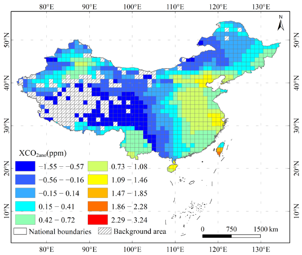
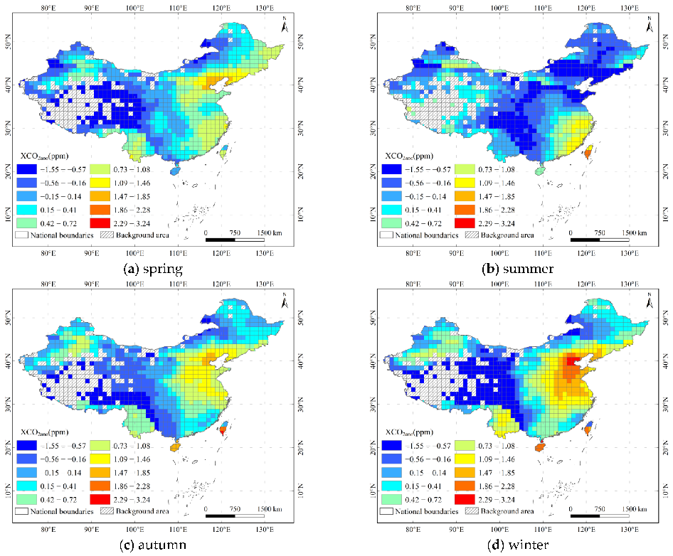
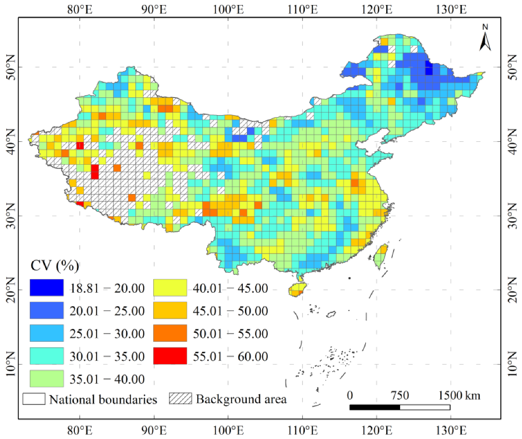
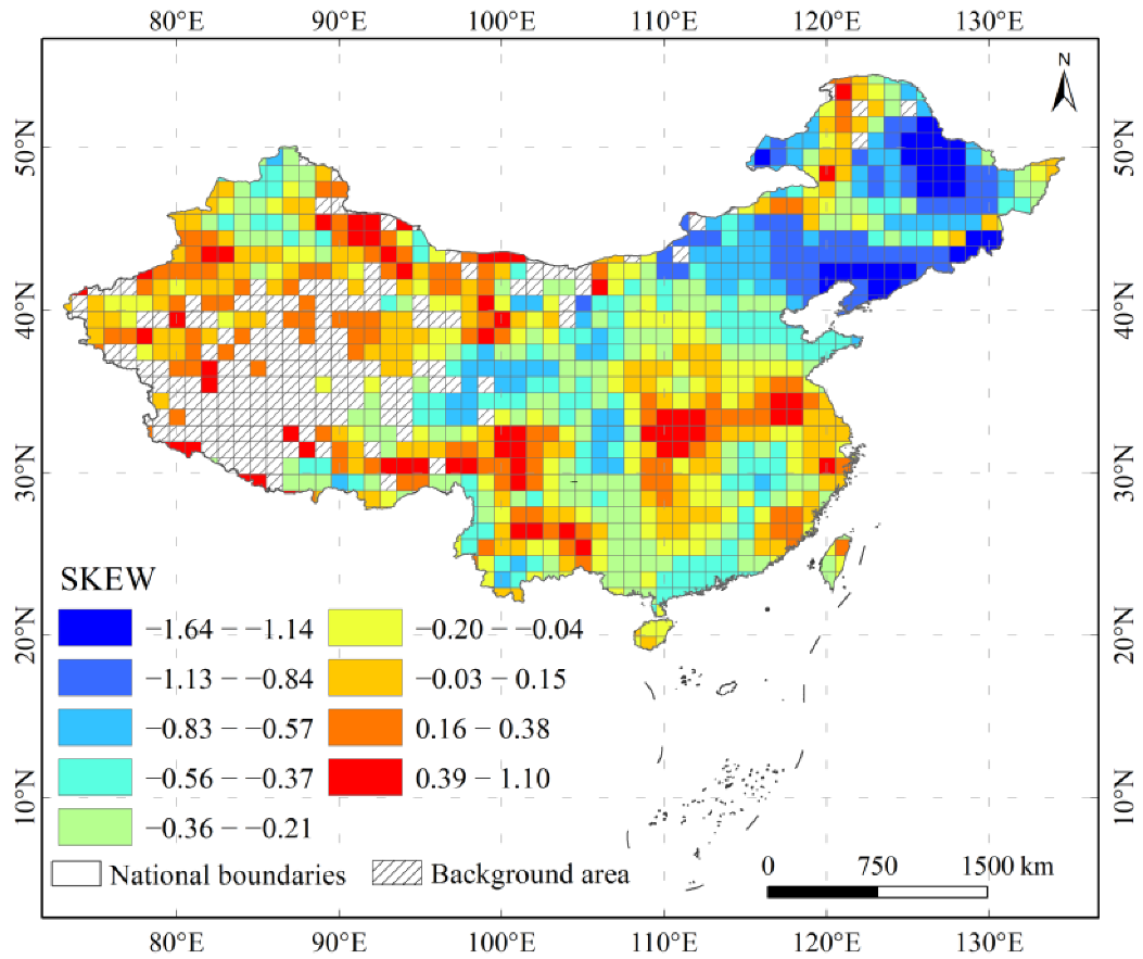
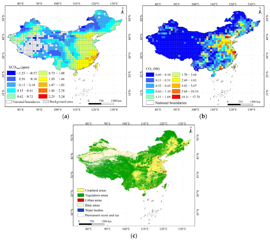
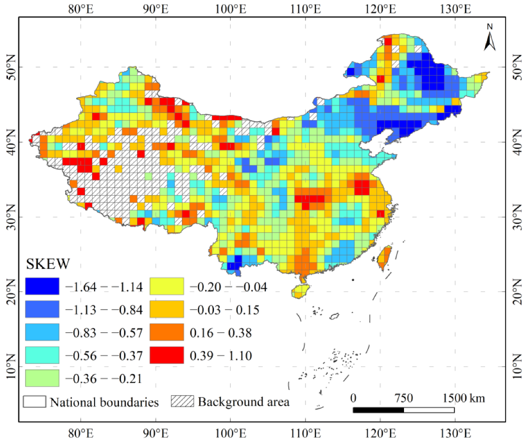
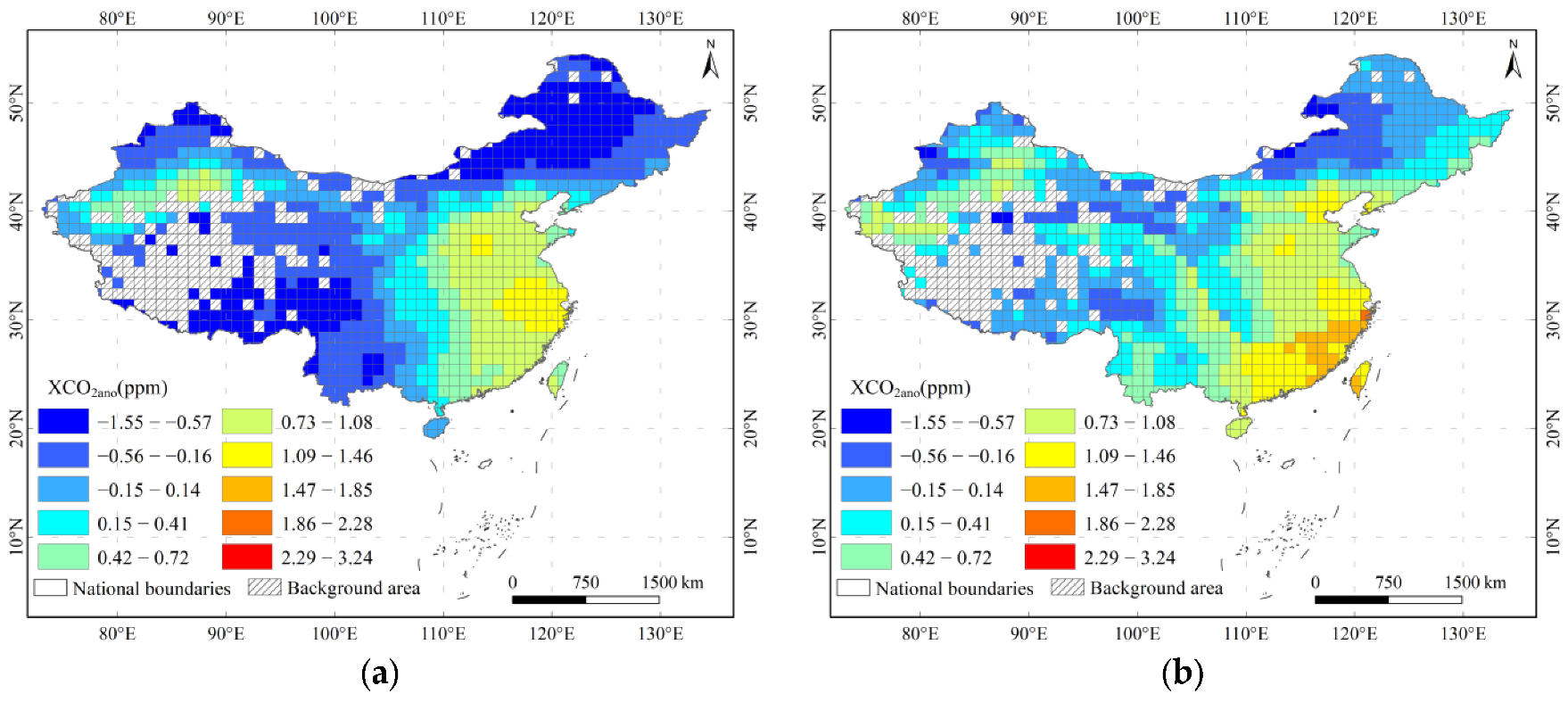
3.1. Characteristics of Spatiotemporal Distribution in XCO_2ano

In this study, the spatial distribution of monthly average XCO_2ano values from 2010 to 2020 was calculated (Figure 4), and the results showed that the overall spatial distribution pattern of XCO_2ano values in China was similar to the spatial distribution pattern of fossil fuel emissions from ODIAC data. The high-value areas of China’s XCO_2ano are mainly distributed in the Yangtze River Delta, the Pearl River Delta, and the Beijing–Tianjin–Hebei urban agglomeration. The areas around these three urban agglomerations also have high XCO_2ano values. The low-value areas of China’s XCO_2ano are mainly distributed in western China. However, there is a high XCO_2ano in the economically underdeveloped Xinjiang. Some studies believe that Xinjiang’s anthropogenic carbon emissions should be less, and the results are more uncertain due to the small number of satellite observations [31,37]. In fact, statistics show that energy consumption in Xinjiang is at a relatively high level [44,45]. Therefore, XCO_2ano high in Xinjiang is consistent with actual anthropogenic carbon emissions. The spatial distribution of monthly average XCO_2ano values from 2010 to 2020 was calculated with the background without the high altitudes is shown in Appendix A Figure A1.

The results show that there are obvious differences between XCO_2ano and ODIAC data in the Yangtze River Delta. Combined with land use data, it can be found that the differences are located in the southern area near urban land, mainly because local atmospheric transport may cause anthropogenic carbon emissions in the Yangtze River Delta region to be transported to the south, resulting in differences. There are also obvious differences between XCO_2ano and ODIAC data in the Pearl River Delta region and Northeast China. In addition to the diffusion of anthropogenic carbon emissions due to atmospheric transport, the rich vegetation resources around the Pearl River Delta and northeastern China will absorb a large amount of anthropogenic carbon emissions, resulting in differences.

To analyze the inter-annual variability of XCO_2ano in China, this study selected the XCO_2ano in 2010, 2015, and 2020 for spatial variability analysis (Figure 5). The results show that the XCO_2ano in 2020 is significantly higher than that of the other two years. Although there were spatial differences in the XCO_2ano in the three years, the high values of XCO_2ano in the three years were mainly distributed in the southeast coastal areas, and the low values of XCO_2ano were mainly distributed in the west and northeast regions. The spatial distribution results of XCO_2ano for the remaining years in China from 2010 to 2020 are shown in Appendix A Figure A2. Although there are obvious changes in XCO_2ano in China from 2010 to 2020, XCO_2ano in coastal areas of China has always maintained a high level. The spatial distribution results of XCO_2ano were calculated with the background without the high altitudes from 2010 to 2020 are shown in Appendix A Figure A3.

In addition, to analyze the seasonality of the XCO_2ano in China, this study plotted the spatial distribution of the average XCO_2ano of four seasons (Spring: March–May; Summer: June to August; Autumn: September–November; Winter: December to February) from 2010 to 2020 (Figure 6). The results show that the XCO_2ano in China has obvious seasonality. The XCO_2ano in winter is higher than that in the other three seasons, plant photosynthesis is the weakest in winter, and heating in winter increases the use of fossil fuels so that there is a higher XCO_2ano in winter. In summer, plant photosynthesis is the strongest, and the terrestrial ecosystem absorbs a large amount of the anthropogenic carbon emissions, so the XCO_2ano in summer is lower than that in the other three seasons, and the XCO_2ano in spring and autumn is between summer and winter. Although there were differences in the spatial distribution of XCO_2ano in the four seasons, they all had similar spatial distribution patterns. Due to the influence of vegetation photosynthesis and other factors, the seasonal variation of XCO_2ano cannot show the same seasonal variation of anthropogenic carbon emissions. If carbon sink information is subsequently added, XCO_2ano can be better linked to anthropogenic carbon emissions. The spatial distribution of the average XCO_2ano of four seasons was calculated with the background without the high altitudes from 2010 to 2020 are shown in Appendix A Figure A4.

To better analyze the seasonal variation in the XCO_2ano in China, this study calculated the monthly average monthly value of the XCO_2ano in different potential temperature zones (Figure 7). The results showed that the XCO_2ano in different potential temperature zones showed obvious seasonal changes, with the highest XCO_2ano in winter and the lowest XCO_2ano in summer (which even contained negative values). The negative value exists more in summer because vegetation photosynthesis strongly absorbs anthropogenic carbon emissions in summer. According to formula 1, the CO₂ absorbed by vegetation photosynthesis in the emission area is higher than that in the background area, which may lead to negative XCO_2ano. If carbon sink information can be added later, we can better eliminate the effect of vegetation photosynthesis. However, XCO_2ano in some years of area I showed an opposite time trend, such as 2012, 2013, and 2019, which showed negative peaks in winter.

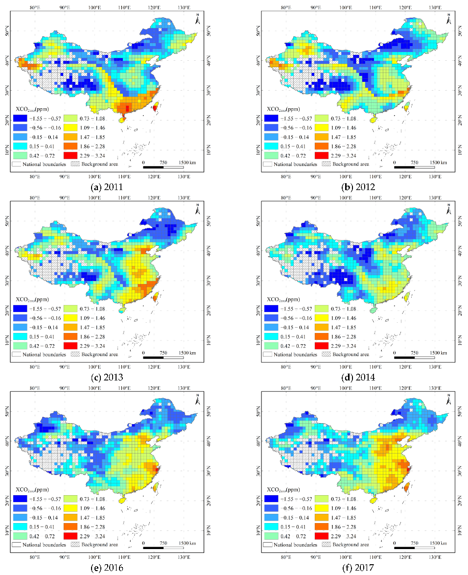
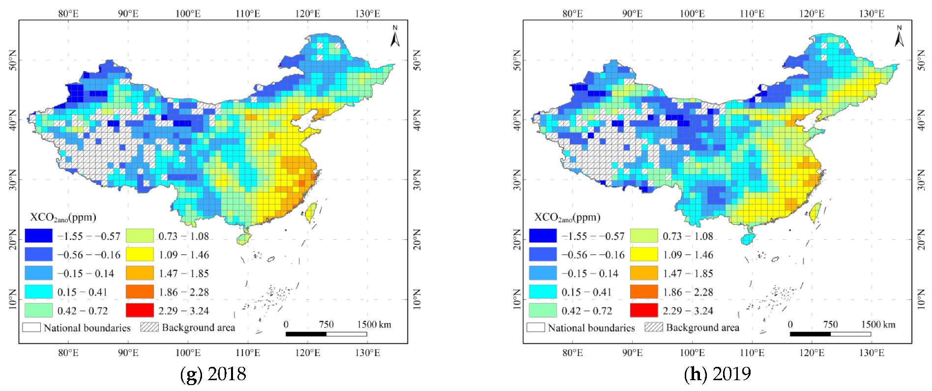
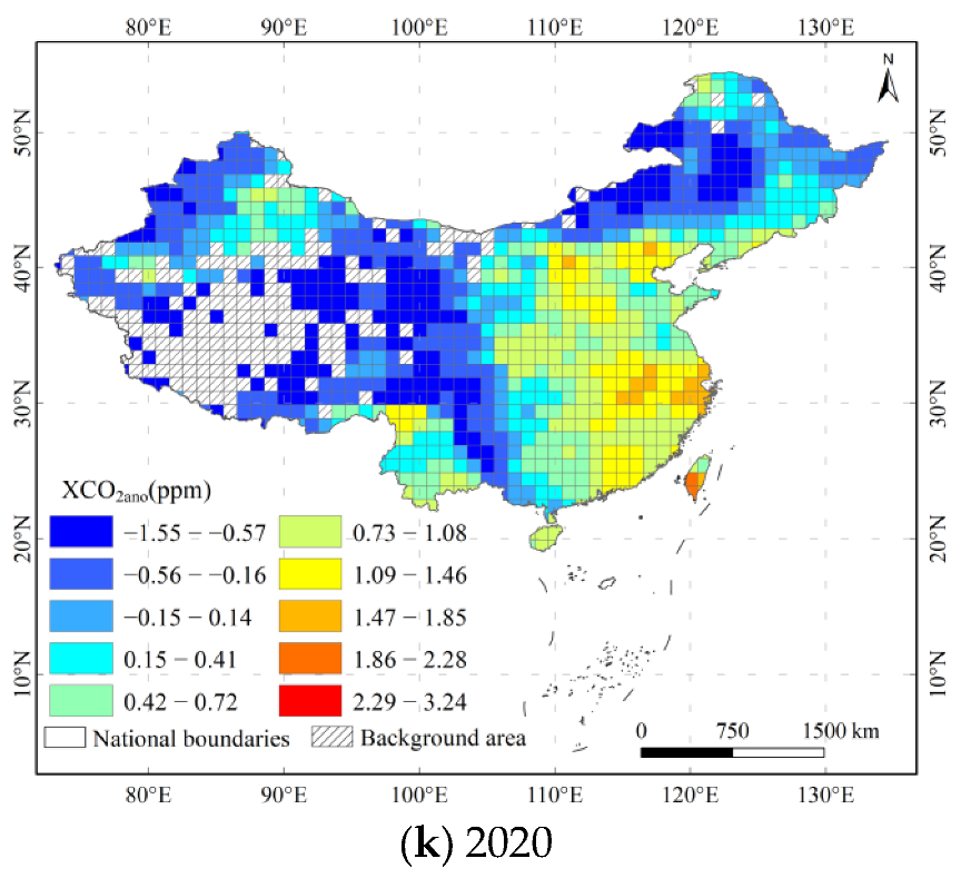
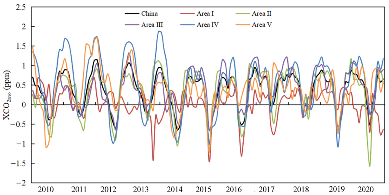
3.2. Spatiotemporal Variation of the XCO_2ano

To analyze the spatiotemporal trends of the XCO_2ano in China, this study calculated the coefficient of variation of the XCO_2ano in China from 2010 to 2020 (Figure 8). The CV can reflect the magnitude of the change in XCO_2ano. The results showed that the of XCO_2ano in China changed greatly from 2010 to 2020, with an average CV of 36.16%. The average CV of area III and area IV was larger, 37.74% and 38.85%, respectively, while the average CV of area I was smaller, only 30.10%, and the average coefficients of variation of area II and area V were 35.06% and 34.48%, respectively. The average CV of the five regions was all higher than 30%, indicating that China’s XCO_2ano changed greatly during 2010–2020. The areas with large changes in XCO_2ano in China are mainly distributed in the Yangtze River Delta urban agglomeration and western China located in area III and area IV, and the XCO_2ano in northeastern China located in area I and Yunnan Province in area V has small changes. XCO_2ano contains anthropogenic carbon emission signals, which are generated by human production and life. Therefore, the change degree of XCO_2ano has a certain relationship with social and economic development. We can find that regions III and IV with high average CV include the Pearl River Delta and the Yangtze River Delta, which are the most economically active regions in China, while region I with low average CV is mainly located in northeast China, which has slow economic development. The coefficient of variation of the XCO_2ano from 2010 to 2020 was calculated with the background without the high altitudes are shown in Appendix A Figure A5.

In addition, this study calculated the SKEW of the XCO_2ano in China from 2010 to 2020 (Figure 9). SKEW can reflect the change direction of the XCO_2ano. The results show that the SKEW of the XCO_2ano in most areas of China from 2010 to 2020 is less than 0, and the average SKEW is −0.26, indicating that the high value of the XCO_2ano in most areas of China is biased toward the end of the time series, and the overall XCO_2ano in China is increasing. The average SKEWs of area I and area II are smaller, −0.53 and −0.52, respectively. The average SKEWs of area III, area IV, and area V are similar, −0.12, −0.11, and −0.19, respectively. The variation coefficient of the XCO_2ano in Northeast China located in area I is relatively small, indicating that although the variation in the XCO_2ano in Northeast China is small, it is in a significant increasing trend. In addition, there are many cases of positive SKEWs in China, indicating that in 2010–2020, the high value of the XCO_2ano in China is more inclined towards the start of the time series. For the region with significant growth of XCO_2ano, it is necessary to consider improving the regional low-carbon production capacity, adjusting the energy structure and improving energy utilization efficiency to control carbon emissions. The SKEW of the XCO_2ano from 2010 to 2020 was calculated with the background without the high altitudes are shown in Appendix A Figure A6.

In addition, the CV and SKEW of XCO_2ano in China also have seasonality. In this study, the average CV and average SKEW of the XCO_2ano in China in the four seasons were calculated (

Table 2. Seasonal difference in CV and SKEW.

Coefficient	Annual	Spring	Summer	Autumn	Winter
CV	36.16	27.94	44.91	29.08	25.64
SKEW	−0.26	−0.01	−0.14	−0.04	−0.06

). The results show that the CV in winter is the smallest, and the CV in summer is significantly larger than that in the other three seasons. Summer is the season where photosynthesis in plants is most obvious, and it is also a season with large changes in meteorological conditions. Therefore, there will be obvious differences in the meteorological conditions in the three months of summer, so that not only the internal summer XCO_2ano is different but also different months in summer in the same year, resulting in an excessively large CV in summer. Compared with summer, the effect of photosynthesis in winter is weaker, and the meteorological conditions are relatively more stable, so XCO_2ano in winter can better reflect anthropogenic carbon emissions. The SKEWs of the four seasons are all less than 0, among which the SKEW is the smallest in summer, indicating that the XCO_2ano does not only change greatly in summer, but also exhibits an increasing trend. Among them, the anthropogenic carbon emissions increased the fastest in summer and the slowest in spring. The average CV and average SKEW of the XCO_2ano in China in the four seasons were calculated with the background without the high altitudes and are shown in Appendix A

Table A1. Seasonal difference in CV and SKEW of XCO_2ano with the background without the high altitudes.

Coefficient	Annual	Spring	Summer	Autumn	Winter
CV	36.34	29.58	41.04	29.46	30.14
SKEW	−0.28	−0.02	−0.12	−0.11	−0.17

.

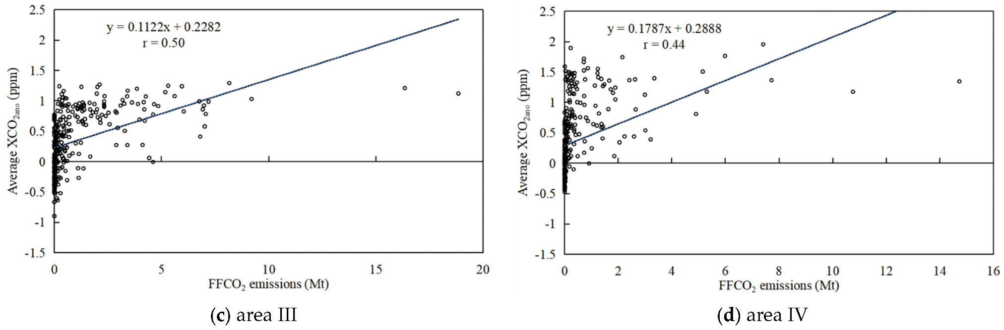
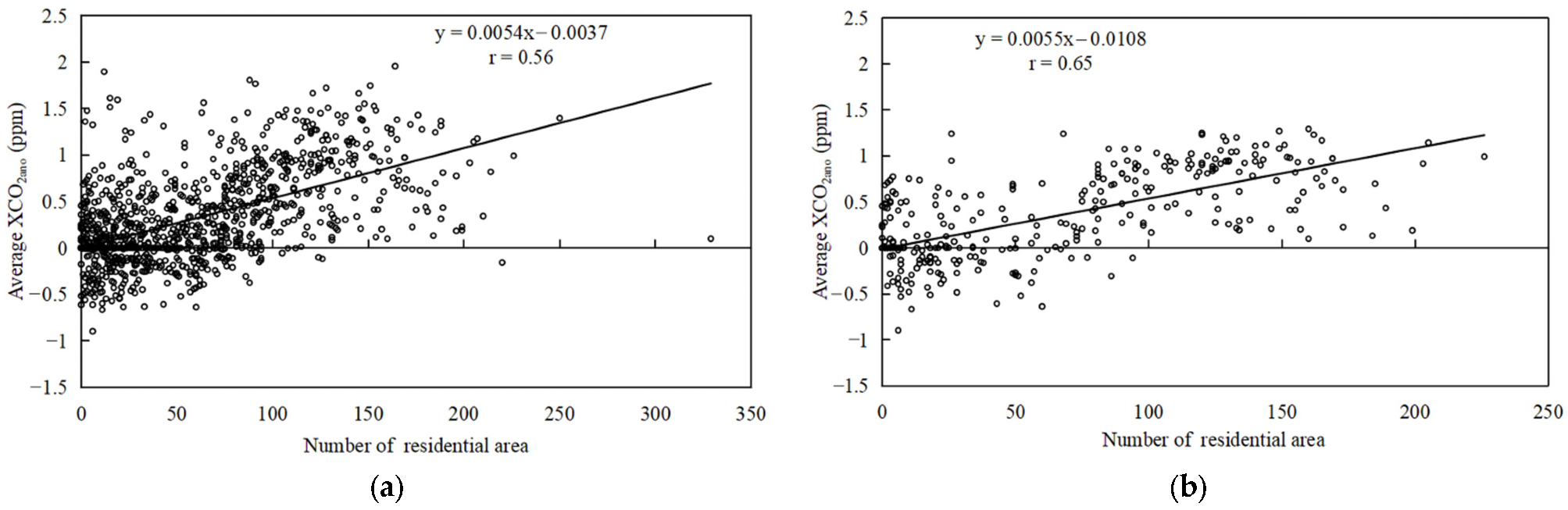
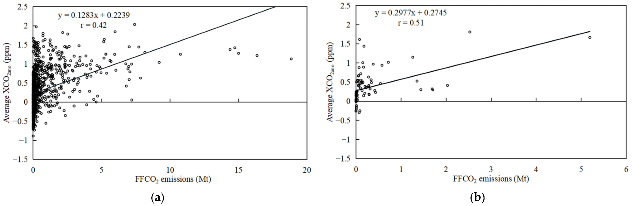
3.3. Correlation Analysis of XCO_2ano

In this study, the regional comparison method was used to calculate the XCO_2ano in the emission area. The anthropogenic carbon emissions in the emission area have a cumulative effect on the XCO₂, so XCO_2ano has a positive correlation with the number of residential areas (Figure 10). The results show that there is a certain positive correlation between the XCO_2ano in China and the number of residential areas but the correlation is low. In addition, this study analyzes the correlation between the XCO_2ano and the number of residential areas in different potential temperature zones. Among them, in Area III, the two have the strongest positive correlation. Area III includes not only economically developed Yangtze River Delta and Beijing–Tianjin–Hebei urban agglomerations but also economically underdeveloped western China. The correlation analysis of average XCO_2ano and the number of residential areas for the other four areas is in Appendix A Figure A7.

The purpose of calculating the XCO_2ano through satellite observations is to monitor and track anthropogenic carbon emissions. In this study, the correlation between the average XCO_2ano and fossil fuel emissions was analyzed. The results show that there is only a weak positive correlation between the two (Figure 11). In Area V, the two have the strongest positive correlation, but the correlation coefficient r is only 0.51, mainly because there is a nonlinear relationship between the XCO_2ano and fossil fuel emissions, and the XCO_2ano is also affected by terrestrial ecosystems and atmospheric transport [35]. Therefore, the XCO_2ano does not only reflect anthropogenic carbon emissions, but is also affected by plant photosynthesis and wind transport. There are many cases where the XCO_2ano overestimates fossil fuel emissions. Atmospheric transport will transport some of the fossil fuel emissions to the surrounding areas, enhancing the XCO₂ observed by satellites in the surrounding areas. The underestimation is mainly due to the absorption of some anthropogenic carbon emissions by plant photosynthesis. The correlation analysis of average XCO_2ano and fossil fuel emissions for the other four areas is in Appendix A Figure A8.

4. Discussion

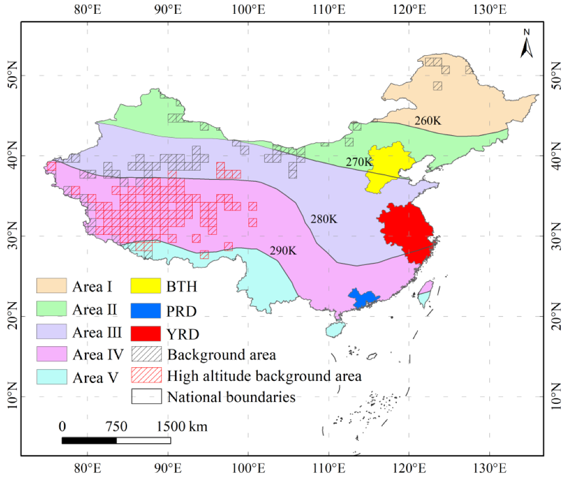
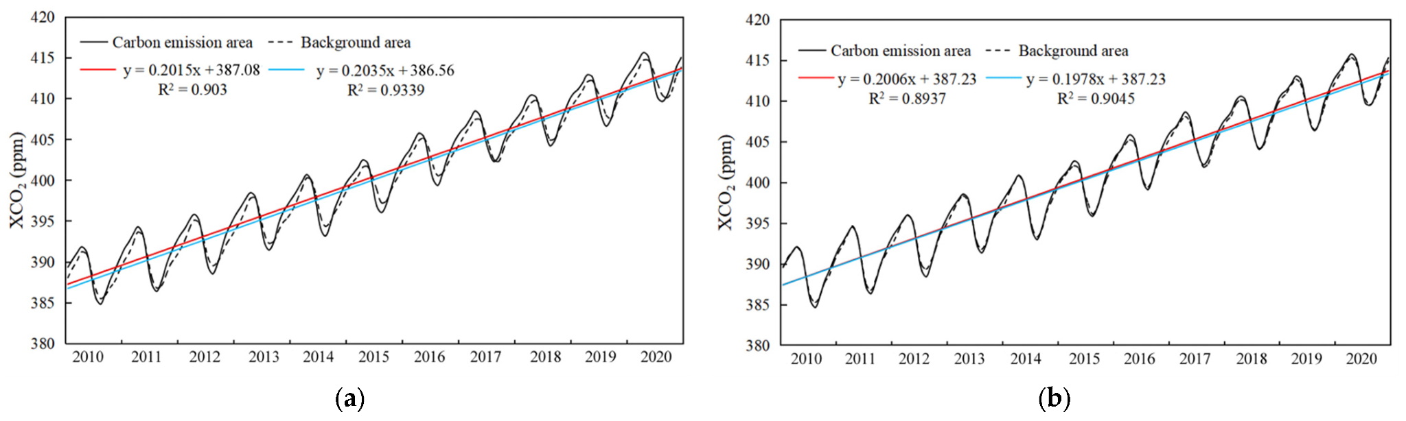
4.1. Selection of Background Area

The XCO₂ in the background area of different potential temperature partitions has some differences. According to the XCO_2ano calculation method of Formula (1), the XCO₂ in the background area will directly affect the XCO_2ano result. The average XCO_2ano in different regions is shown in

Table 3. The average XCO_2ano in different partitions.

Area	Area I	Area II	Area III	Area IV	Area V
Background (ppm)	399.82	399.97	400.62	399.97	399.66
Anthropogenic emission area (ppm)	399.86	400.30	401.91	401.93	401.47
XCO2ano average (ppm)	0.04	0.33	1.29	1.96	1.81

. The results show that the average XCO_2ano in Area I and Area II is lower, and the XCO_2ano in the other three regions is significantly higher. Among them, Area IV has the highest XCO_2ano. Area IV includes the Pearl River Delta urban agglomeration and the Yangtze River Delta urban agglomeration with active economic activities in China. Urban development needs to be driven by energy consumption, which produces anthropogenic carbon emissions that lead to an increase in atmospheric CO₂. Relevant studies have shown that cities are the promoters of the increase in atmospheric CO₂, and their anthropogenic carbon emissions also promote the growth of XCO_2ano [35].

Partitioning according to potential temperature can reduce the influence of atmospheric transport, and there are obvious differences in the background XCO₂ different partitions, so it is necessary to calculate the XCO_2ano by partition. Some related studies have used the idea of zoning and selected the median or average value of XCO₂ in different zones as the background [31,35], while this study chose the average value as the background.

To quantitatively analyze the impact of different background area selection methods on the capturing of anthropogenic carbon emission signals, this study selected the median XCO₂ in China as the background to calculate the XCO_2ano in the anthropogenic carbon emission area (Figure 12a). The results show that the XCO_2ano result cannot better reflect the spatial distribution pattern of China’s anthropogenic carbon emissions. In addition, the median XCO₂ value in five zones was extracted according to the background area determined in this study and the XCO_2ano was calculated (Figure 12b). The results show that the XCO_2ano results are similar to the spatial distribution pattern of this study.

To quantify the potential of selecting median and average XCO₂ as background value to monitor anthropogenic carbon emissions, this study also performed a correlation analysis between the above XCO_2ano results and fossil fuel emissions (Figure 13). The results show that the correlations between the XCO_2ano and fossil fuel emissions using the Chinese median XCO₂ and the regional median XCO_2ano as the background are 0.40 and 0.42, respectively. This is lower than the correlation coefficient between the XCO_2ano and fossil fuel emissions as determined in this study (Figure 11a). Therefore, choosing the average XCO₂ can improve the monitoring of anthropogenic carbon emissions. Most previous studies chose the median XCO₂ for subsequent XCO_2ano calculation. The selection of median can remove the influence of outliers, but for the small area of this study, it may cause information omission.

4.2. Uncertainty Factor Analysis of the XCO_2ano

Compared to bottom-up anthropogenic emissions inventory data, satellite observations are susceptible to meteorological, biological, and atmospheric conditions. The area explored in this study is large, and the wind field in a small area still interferes with the anthropogenic carbon emission signal in the XCO_2ano. Wind farms can diffuse CO₂ from anthropogenic sources to surrounding areas. XCO₂ over high altitude points has a less pronounced seasonal cycle. As shown in Figure 3b, the problem of higher XCO₂ values in the background area than in the emission area in summer largely disappears after removing the high altitude background points. (except for years 2010 and 2012). At present, WRF modelled wind field/wind measurements from LiDAR equipment has been widely used, among which Doppler wind LiDAR is a relatively new technology to acquire wind measurement [46]. In the future, relevant technologies can be considered to eliminate the influence of wind field. In addition, the XCO_2ano also includes the effect of biological sinks. Using only deserts or bare land as background to compare with vegetated emission areas causes a strong low bias in the emission effect because of removal of CO₂ by photosynthesis. We will work on this in a subsequent study. This is especially true in summer when the photosynthesis of plants absorbs a large amount of CO₂ and makes the correlation between XCO_2ano and fossil fuel emissions weaker. Subsequent auxiliary data related to CO₂ absorption and emissions should be added to enhance anthropogenic carbon emissions signals, such as net primary productivity and nighttime light images, to enhance the ability of satellite observations to assess and monitor anthropogenic carbon emissions. At the same time, satellites are sensitive to clouds and aerosols, resulting in relatively little available data in some areas [47]. Thus, satellite observations will have greater uncertainty [48].

4.3. Discussion on the Accurate Monitoring of Anthropogenic Carbon Emission

This study calculated the XCO_2ano in China based on satellite observation data, but there are some remaining shortcomings. The goal of the study is to monitor and evaluate anthropogenic carbon emissions. The results show that the XCO_2ano in this study has only a weak correlation with the fossil fuel emissions of the ODIAC data. The issue of how to solve the influence of biological and atmospheric factors is the main focus of subsequent research. Future research will consider adding data related to carbon absorption and carbon emissions such as vegetation index and solar-induced chlorophyll fluorescence. In addition, regional carbon neutrality is also an ecological issue of social concern, and subsequent studies will analyze the current status of regional carbon neutrality.

5. Conclusions

This study aims to eliminate the influence of uncertainty factors in XCO₂ as far as possible to enhance the anthropogenic carbon emission signal. Based on the regional comparison method based on the idea of zoning, this study uses the potential temperature data and the ODIAC data set to effectively enhance the anthropogenic carbon emission signal in XCO₂, and strengthen the remote sensing monitoring ability of anthropogenic carbon emission spatiotemporal changes. In this study, 2010–2020 monthly Mapping-XCO₂ data were used to calculate the spatiotemporal distributions of XCO_2ano in China, and the spatiotemporal changes in the results were analyzed. The XCO_2ano in China has obvious spatiotemporal differences. In addition, there are obvious seasonal variations, with the highest XCO_2ano in winter and the lowest in summer. The variation range of XCO_2ano in China is large, and showed an increasing trend, and the variation of XCO_2ano also has seasonality. The XCO_2ano has a high similarity with the spatial distribution of fossil fuel carbon emissions, which provides remote sensing observation means for anthropogenic carbon emissions monitoring. Compared with previous studies, the regional comparison method based on the idea of zoning can better enhance the anthropogenic carbon emission signal in XCO₂, and using the average background regional as the background can better monitor anthropogenic carbon emission.

In order to explore the feasibility of satellite observation for assessing and monitoring anthropogenic carbon emissions, this study combined ODIAC data and potential temperature data to select a regionalized background region, and designed a regional comparison method based on the idea of zoning to eliminate background CO₂ and enhance anthropogenic carbon emission signals in XCO₂. Relevant research results can provide a policy reference for China’s “dual carbon” strategy. The anthropogenic carbon emission in the atmospheric carbon is very low, and the fluctuation caused by it is difficult to accurately measure. With the development of remote sensing technology, it is hoped that carbon monitoring satellites can provide higher-precision XCO₂ data. In the future, we will add CO₂-related data for background region selection and supplement carbon neutrality research.

References

1. Zickfeld, K.; Solomon, S.; Gilford, D.M. Centuries of thermal sea-level rise due to anthropogenic emissions of short-lived greenhouse gases. Proc. Natl. Acad. Sci. USA 2017, 114, 657–662. [Google Scholar] [CrossRef] [PubMed] [Green Version]
2. Jin, T.; Kim, J. What is better for mitigating carbon emissions—Renewable energy or nuclear energy? A panel data analysis. Renew. Sustain. Energy Rev. 2018, 91, 464–471. [Google Scholar] [CrossRef]
3. Dai, A.; Luo, D.; Song, M.; Liu, J. Arctic amplification is caused by sea-ice loss under increasing CO2. Nat. Commun. 2019, 10, 121. [Google Scholar] [CrossRef] [Green Version]
4. Wu, Y.; Tam, V.W.Y.; Shuai, C.; Shen, L.; Zhang, Y.; Liao, S. Decoupling China’s economic growth from carbon emissions: Empirical studies from 30 Chinese provinces (2001–2015). Sci. Total Environ. 2019, 656, 576–588. [Google Scholar] [CrossRef] [PubMed]
5. Peters, G.P.; Le Quéré, C.; Andrew, R.M.; Canadell, J.G.; Friedlingstein, P.; Ilyina, T.; Jackson, R.B.; Joos, F.; Korsbakken, J.I.; McKinley, G.A.; et al. Towards real-time verification of CO2 emissions. Nat. Clim. Change 2017, 7, 848–850. [Google Scholar] [CrossRef] [Green Version]
6. Jiang, J.; Ye, B.; Liu, J. Research on the peak of CO2 emissions in the developing world: Current progress and future prospect. Appl. Energy 2019, 235, 186–203. [Google Scholar] [CrossRef]
7. Friedlingstein, P.; O’Sullivan, M.; Jones, M.W.; Andrew, R.M.; Hauck, J.; Olsen, A.; Peters, G.P.; Peters, W.; Pongratz, J.; Sitch, S.; et al. Global Carbon Budget 2020. Earth Syst. Sci. Data 2020, 12, 3269–3340. [Google Scholar] [CrossRef]
8. IPCC. Climate Change 2014: Synthesis Report. Contribution of Rorking Groups I, II and III to the Fifth Assessment Report of the Intergovernmental Panel on Climate Change; Pachauri, R.K., Meyer, L.A., Eds.; IPCC: Geneva, Switzerland, 2014.
9. Khan, Y.; Hassan, T.; Kirikkaleli, D.; Xiuqin, Z.; Shukai, C. The impact of economic policy uncertainty on carbon emissions: Evaluating the role of foreign capital investment and renewable energy in East Asian economies. Environ. Sci. Pollut. Res. Int. 2022, 29, 18527–18545. [Google Scholar] [CrossRef]
10. Labzovskii, L.D.; Mak, H.W.L.; Takele Kenea, S.; Rhee, J.-S.; Lashkari, A.; Li, S.; Goo, T.-Y.; Oh, Y.-S.; Byun, Y.-H. What can we learn about effectiveness of carbon reduction policies from interannual variability of fossil fuel CO2 emissions in East Asia? Environ. Sci. Policy 2019, 96, 132–140. [Google Scholar] [CrossRef]
11. Rogelj, J.; den Elzen, M.; Hohne, N.; Fransen, T.; Fekete, H.; Winkler, H.; Schaeffer, R.; Sha, F.; Riahi, K.; Meinshausen, M. Paris Agreement climate proposals need a boost to keep warming well below 2 °C. Nature 2016, 534, 631–639. [Google Scholar] [CrossRef] [Green Version]
12. Chen, J.; Wang, L.; Li, Y. Research on the impact of multi-dimensional urbanization on China’s carbon emissions under the background of COP21. J. Environ. Manag. 2020, 273, 111123. [Google Scholar] [CrossRef]
13. Jiang, T.; Yu, Y.; Jahanger, A.; Balsalobre-Lorente, D. Structural emissions reduction of China’s power and heating industry under the goal of “double carbon”: A perspective from input-output analysis. Sustain. Prod. Consum. 2022, 31, 346–356. [Google Scholar] [CrossRef]
14. Wei, Y.-M.; Chen, K.; Kang, J.-N.; Chen, W.; Wang, X.-Y.; Zhang, X. Policy and Management of Carbon Peaking and Carbon Neutrality: A Literature Review. Engineering 2022, 14, 52–63. [Google Scholar] [CrossRef]
15. Zhao, X.; Ma, X.; Chen, B.; Shang, Y.; Song, M. Challenges toward carbon neutrality in China: Strategies and countermeasures. Resour. Conserv. Recycl. 2022, 176, 105959. [Google Scholar] [CrossRef]
16. Xu, Q.; Dong, Y.-X.; Yang, R.; Zhang, H.-O.; Wang, C.-J.; Du, Z.-W. Temporal and spatial differences in carbon emissions in the Pearl River Delta based on multi-resolution emission inventory modeling. J. Clean. Prod. 2019, 214, 615–622. [Google Scholar] [CrossRef]
17. Liu, Z.; Guan, D.; Wei, W.; Davis, S.J.; Ciais, P.; Bai, J.; Peng, S.; Zhang, Q.; Hubacek, K.; Marland, G.; et al. Reduced carbon emission estimates from fossil fuel combustion and cement production in China. Nature 2015, 524, 335–338. [Google Scholar] [CrossRef] [Green Version]
18. Zheng, J.; Mi, Z.; Coffman, D.M.; Milcheva, S.; Shan, Y.; Guan, D.; Wang, S. Regional development and carbon emissions in China. Energy Econ. 2019, 81, 25–36. [Google Scholar] [CrossRef]
19. Khan, Z.; Ali, S.; Umar, M.; Kirikkaleli, D.; Jiao, Z. Consumption-based carbon emissions and International trade in G7 countries: The role of Environmental innovation and Renewable energy. Sci. Total Environ. 2020, 730, 138945. [Google Scholar] [CrossRef]
20. Zhang, W.; Li, J.; Li, G.; Guo, S. Emission reduction effect and carbon market efficiency of carbon emissions trading policy in China. Energy 2020, 196, 117117. [Google Scholar] [CrossRef]
21. Wunch, D.; Toon, G.C.; Blavier, J.F.; Washenfelder, R.A.; Notholt, J.; Connor, B.J.; Griffith, D.W.; Sherlock, V.; Wennberg, P.O. The total carbon column observing network. Philos. Trans. A Math. Phys. Eng. Sci. 2011, 369, 2087–2112. [Google Scholar] [CrossRef] [Green Version]
22. Duren, R.M.; Miller, C.E. Measuring the carbon emissions of megacities. Nat. Clim. Change 2012, 2, 560–562. [Google Scholar] [CrossRef]
23. Hochstaffl, P.; Schreier, F.; Lichtenberg, G.; Gimeno García, S. Validation of Carbon Monoxide Total Column Retrievals from SCIAMACHY Observations with NDACC/TCCON Ground-Based Measurements. Remote Sens. 2018, 10, 223. [Google Scholar] [CrossRef] [Green Version]
24. Shi, K.; Xu, T.; Li, Y.; Chen, Z.; Gong, W.; Wu, J.; Yu, B. Effects of urban forms on CO2 emissions in China from a multi-perspective analysis. J. Environ. Manag. 2020, 262, 110300. [Google Scholar] [CrossRef] [PubMed]
25. Buchwitz, M.; Reuter, M.; Schneising, O.; Boesch, H.; Guerlet, S.; Dils, B.; Aben, I.; Armante, R.; Bergamaschi, P.; Blumenstock, T.; et al. The Greenhouse Gas Climate Change Initiative (GHG-CCI): Comparison and quality assessment of near-surface-sensitive satellite-derived CO2 and CH4 global data sets. Remote Sens. Environ. 2015, 162, 344–362. [Google Scholar] [CrossRef] [Green Version]
26. Wunch, D.; Wennberg, P.O.; Osterman, G.; Fisher, B.; Naylor, B.; Roehl, C.M.; O’Dell, C.; Mandrake, L.; Viatte, C.; Kiel, M.; et al. Comparisons of the Orbiting Carbon Observatory-2 (OCO-2) XCO2 measurements with TCCON. Atmos. Meas. Tech. 2017, 10, 2209–2238. [Google Scholar] [CrossRef] [Green Version]
27. Zheng, T.; Nassar, R.; Baxter, M. Estimating power plant CO2 emission using OCO-2 XCO2 and high resolution WRF-Chem simulations. Environ. Res. Lett. 2019, 14, 085001. [Google Scholar] [CrossRef]
28. Boesch, H.; Liu, Y.; Tamminen, J.; Yang, D.; Palmer, P.I.; Lindqvist, H.; Cai, Z.; Che, K.; Di Noia, A.; Feng, L.; et al. Monitoring Greenhouse Gases from Space. Remote Sens. 2021, 13, 2700. [Google Scholar] [CrossRef]
29. Hakkarainen, J.; Ialongo, I.; Maksyutov, S.; Crisp, D. Analysis of Four Years of Global XCO2 Anomalies as Seen by Orbiting Carbon Observatory-2. Remote Sens. 2019, 11, 850. [Google Scholar] [CrossRef] [Green Version]
30. Mustafa, F.; Bu, L.; Wang, Q.; Yao, N.; Shahzaman, M.; Bilal, M.; Aslam, R.W.; Iqbal, R. Neural-network-based estimation of regional-scale anthropogenic CO2 emissions using an Orbiting Carbon Observatory-2 (OCO-2) dataset over East and West Asia. Atmos. Meas. Tech. 2021, 14, 7277–7290. [Google Scholar] [CrossRef]
31. Sheng, M.; Lei, L.; Zeng, Z.-C.; Rao, W.; Zhang, S. Detecting the Responses of CO2 Column Abundances to Anthropogenic Emissions from Satellite Observations of GOSAT and OCO-2. Remote Sens. 2021, 13, 3524. [Google Scholar] [CrossRef]
32. Wang, H.; Gong, F.-Y.; Newman, S.; Zeng, Z.-C. Consistent weekly cycles of atmospheric NO2, CO, and CO2 in a North American megacity from ground-based, mountaintop, and satellite measurements. Atmos. Environ. 2022, 268, 118809. [Google Scholar] [CrossRef]
33. Lu, S.; Wang, J.; Wang, Y.; Yan, J. Analysis on the variations of atmospheric CO2 concentrations along the urban–rural gradients of Chinese cities based on the OCO-2 XCO2 data. Int. J. Remote Sens. 2018, 39, 4194–4213. [Google Scholar] [CrossRef]
34. Shim, C.; Han, J.; Henze, D.K.; Yoon, T. Identifying local anthropogenic CO2 emissions with satellite retrievals: A case study in South Korea. Int. J. Remote Sens. 2018, 40, 1011–1029. [Google Scholar] [CrossRef] [Green Version]
35. Labzovskii, L.D.; Jeong, S.-J.; Parazoo, N.C. Working towards confident spaceborne monitoring of carbon emissions from cities using Orbiting Carbon Observatory-2. Remote Sens. Environ. 2019, 233, 111359. [Google Scholar] [CrossRef]
36. Buchwitz, M.; Reuter, M.; Noël, S.; Bramstedt, K.; Schneising, O.; Hilker, M.; Fuentes Andrade, B.; Bovensmann, H.; Burrows, J.P.; Di Noia, A.; et al. Can a regional-scale reduction of atmospheric CO2 during the COVID-19 pandemic be detected from space? A case study for East China using satellite XCO2 retrievals. Atmos. Meas. Tech. 2021, 14, 2141–2166. [Google Scholar] [CrossRef]
37. Yang, S.; Lei, L.; Zeng, Z.; He, Z.; Zhong, H. An Assessment of Anthropogenic CO2 Emissions by Satellite-Based Observations in China. Sensors 2019, 19, 1118. [Google Scholar] [CrossRef] [Green Version]
38. He, Z.; Lei, L.; Zhang, Y.; Sheng, M.; Wu, C.; Li, L.; Zeng, Z.-C.; Welp, L.R. Spatio-Temporal Mapping of Multi-Satellite Observed Column Atmospheric CO2 Using Precision-Weighted Kriging Method. Remote Sens. 2020, 12, 576. [Google Scholar] [CrossRef] [Green Version]
39. Sheng, M.; Lei, L.; Zeng, Z.-C.; Rao, W.; Song, H.; Wu, C. Global land 1° mapping dataset of XCO2 from satellite observations of GOSAT and OCO-2 from 2009 to 2020. Big Earth Data 2022, 7, 170–190. [Google Scholar] [CrossRef]
40. Oda, T.; Maksyutov, S. A very high-resolution (1 km × 1 km) global fossil fuel CO2 emission inventory derived using a point source database and satellite observations of nighttime lights. Atmos. Chem. Phys. 2011, 11, 543–556. [Google Scholar] [CrossRef] [Green Version]
41. Oda, T.; Maksyutov, S.; Andres, R.J. The Open-source Data Inventory for Anthropogenic Carbon dioxide (CO2), version 2016 (ODIAC2016): A global, monthly fossil-fuel CO2 gridded emission data product for tracer transport simulations and surface flux inversions. Earth Syst. Sci. Data 2018, 10, 87–107. [Google Scholar] [CrossRef] [Green Version]
42. Keppel-Aleks, G.; Wennberg, P.O.; Schneider, T. Sources of variations in total column carbon dioxide. Atmos. Chem. Phys. 2011, 11, 3581–3593. [Google Scholar] [CrossRef] [Green Version]
43. Keppel-Aleks, G.; Wennberg, P.O.; O’Dell, C.W.; Wunch, D. Towards constraints on fossil fuel emissions from total column carbon dioxide. Atmos. Chem. Phys. 2013, 13, 4349–4357. [Google Scholar] [CrossRef] [Green Version]
44. Xia, F.; Zhang, X.; Cai, T.; Wu, S.; Zhao, D. Identification of key industries of industrial sector with energy-related CO2 emissions and analysis of their potential for energy conservation and emission reduction in Xinjiang, China. Sci. Total Environ. 2020, 708, 134587. [Google Scholar] [CrossRef] [PubMed]
45. Ziyuan, C.; Yibo, Y.; Simayi, Z.; Shengtian, Y.; Abulimiti, M.; Yuqing, W. Carbon emissions index decomposition and carbon emissions prediction in Xinjiang from the perspective of population-related factors, based on the combination of STIRPAT model and neural network. Environ. Sci. Pollut. Res. Int. 2022, 29, 31781–31796. [Google Scholar] [CrossRef]
46. Liu, Z.; Barlow, J.F.; Chan, P.-W.; Fung, J.C.H.; Li, Y.; Ren, C.; Mak, H.W.L.; Ng, E. A Review of Progress and Applications of Pulsed Doppler Wind LiDARs. Remote Sens. 2019, 11, 2522. [Google Scholar] [CrossRef] [Green Version]
47. Vasilkov, A.; Krotkov, N.; Yang, E.-S.; Lamsal, L.; Joiner, J.; Castellanos, P.; Fasnacht, Z.; Spurr, R. Explicit and consistent aerosol correction for visible wavelength satellite cloud and nitrogen dioxide retrievals based on optical properties from a global aerosol analysis. Atmos. Meas. Tech. 2021, 14, 2857–2871. [Google Scholar] [CrossRef]
48. Sanghavi, S.; Nelson, R.; Frankenberg, C.; Gunson, M. Aerosols in OCO-2/GOSAT retrievals of XCO2: An information content and error analysis. Remote Sens. Environ. 2020, 251, 112053. [Google Scholar] [CrossRef]
Figure 1. Partitioning based on potential temperature data. Beijing–Tianjin–Hebei (BTH); Pearl River Delta (PRD); Yangtze River Delta (YRD).
Remotesensing 15 03207 g001
Figure 2. Research flow chart.
Remotesensing 15 03207 g002
Figure 3. Time series of the XCO2. (a) is the time series of XCO2 in the background area and emission area of China, and (b) is the time series of XCO2 in the background area and emission area of China excluding the Tibetan Plateau with an altitude higher than 3000 m. X-axis: January 2010 represents 1, increasing by 1 for every month of growth, and finally December 2020 represents 132.
Remotesensing 15 03207 g003
Figure 4. XCO2ano and ODIAC data fossil fuel emissions spatial distribution and land use data. (a) is the average value of the XCO2ano from 2010 to 2020, (b) is the average value of ODIAC fossil fuel emissions from 2010 to 2019, and (c) is the 300 m spatial resolution land use data.
Remotesensing 15 03207 g004
Figure 5. Spatial distribution of average XCO2ano. (ac) are the spatial distribution of average XCO2ano in China in 2010, 2015 and 2020, respectively.
Remotesensing 15 03207 g005
Figure 6. Spatial distribution of the average XCO2ano. (ad) are the average values of XCO2ano in spring, summer, autumn, and winter from 2010 to 2020, respectively.
Remotesensing 15 03207 g006
Figure 7. Seasonal variation in the mean value of the XCO2ano in five regions and China.
Remotesensing 15 03207 g007
Figure 8. Spatial distribution of the CV of the XCO2ano in China from 2010 to 2020.
Remotesensing 15 03207 g008
Figure 9. Spatial distribution of the SKEW of XCO2ano in China from 2010 to 2020.
Remotesensing 15 03207 g009
Figure 10. The correlation analysis between the average XCO2ano and the number of residential areas, in which (a) is the correlation analysis result of all study areas and (b) is the correlation analysis result of Area III.
Remotesensing 15 03207 g010
Figure 11. Correlation analysis between the average XCO2ano and fossil fuel emissions, in which (a) is the correlation analysis result of all study areas and (b) is the correlation analysis result of Area V.
Remotesensing 15 03207 g011
Figure 12. XCO2ano distribution and average fossil fuel carbon emissions for different background region selection methods. (a) is the XCO2ano obtained with the Chinese median XCO2 is taken as the background value, (b) is the XCO2ano obtained with the regional median XCO2 as the background value.
Remotesensing 15 03207 g012
Figure 13. Correlation analysis of XCO2ano and fossil fuel emissions. (a,b) are the correlations between the XCO2ano and fossil fuel emissions using the Chinese median XCO2 and the regional median XCO2ano as the background value, respectively.
Remotesensing 15 03207 g013