Robust Pedestrian Dead Reckoning Integrating Magnetic Field Signals and Digital Terrestrial Multimedia Broadcasting Signals

Abstract

Currently, many positioning technologies complementary to Global Navigation Satellite System (GNSS) are providing ubiquitous positioning services, especially the coupling positioning of Pedestrian Dead Reckoning (PDR) and other signals. Magnetic field signals are stable and ubiquitous, while Digital Terrestrial Multimedia Broadcasting (DTMB) signals have strong penetration and stable transmission over a large range. To improve the positioning performance of PDR, this paper proposes a robust PDR integrating magnetic field signals and DTMB signals. In our study, the Spiking Neural Network (SNN) is first used to learn the magnetic field signals of the environment, and then the learning model is used to detect the magnetic field landmarks. At the same time, the DTMB signals are collected by the self-developed signal receiver, and then the carrier phase ranging of the DTMB signals is realized. Finally, robust pedestrian positioning is achieved by integrating position information from magnetic field landmarks and ranging information from DTMB signals through Extended Kalman Filter (EKF). We have conducted indoor and outdoor field tests to verify the proposed method, and the outdoor field test results showed that the positioning error cumulative distribution of the proposed method reaches 2.84 m at a 68% probability level, while that of the PDR only reaches 8.77 m. The proposed method has been validated to be effective and has good positioning performance, providing an alternative solution for seamless indoor and outdoor positioning.

1. Introduction

The signal of the Global Navigation Satellite System (GNSS) will be seriously attenuated and blocked in some environments (such as urban canyons, indoors, and underground) [1]. At present, many positioning methods complementary to GNSS have been developed to provide ubiquitous location-based services (LBS). Compared to positioning methods that require the deployment of positioning facilities in advance, such as WiFi [2], Ultra-Wide Band (UWB) [3], Long Term Evolution (LTE) [4], 5G [5], audio [6], etc. Pedestrian Dead Reckoning (PDR) is an independent positioning method. However, due to its sensor characteristics and algorithm design, PDR faces serious challenges of position drift [7].

Magnetic field signals are ubiquitous, and if the environment remains unchanged, they can remain stable for several years [8,9]; it does not require the deployment of base stations and is low-cost. In addition, the magnetic field signals are not affected by multipath effects due to it being a physical field existing on the earth. So, magnetic field signals are effective sources of positioning that can assist PDR. Most of the positioning methods based on magnetic field signals are first to build the magnetic field signal database of the environment in advance and then realize the positioning using the magnetic field signal matching algorithm. Currently, the commonly used matching algorithms include Dynamic Time Warping (DTW) [10], Convolutional Neural Network (CNN) [11], Recurrent Neural Network (RNN) [12], etc. DTW is the most widely used magnetic field signal matching method with small computation and stable positioning performance. CNN has a strong ability for feature extraction of magnetic field signals, while RNN has a strong learning ability for sequence magnetic field signals; however, these existing methods take the magnetic field signal value directly as the input. As the third-generation neural network, Spiking Neural Network (SNN) [13] has the characteristics of event-driven and low-power consumption, and has attracted widespread attention. The neuron model in the traditional neural networks is based on numerical calculation, while SNN transmits information by action potential sequence rather than numerical value, which is a neuromorphological model with biological significance. However, SNN is difficult to train due to its complex neuron dynamics and indistinguishable spike operation. With the development of SNN, research and applications based on SNN are also increasing. Gutig et al. [14] proposed an SNN for classification, called Templeton. This method defined the Leaky Integrate-and-Fire (LIF) neuron model and gave the learning mechanism based on neuron potential. Fang et al. [15] proposed a learning algorithm based on back-propagation using spiking neurons with learnable membrane parameters, called Parameter Leaky Integrate-and-Fire (PLIF) spike neurons. This method better represents the heterogeneity of neurons, thus enhancing the performance of SNN. Kim et al. [16] presented the first spiked-based object detection model, called Spiking-YOLO. The method introduced channel-wise normalization and signed neurons with imbalanced thresholds, both of which provide fast and accurate information transmission for deep SNN, making its detection accuracy up to 98%. Thus far, SNN is mainly used for image classification and object detection. Inspired that the magnetic field sequence signals can be mapped to the image, this paper first proposes using SNN to detect magnetic field landmarks to assist PDR. Nevertheless, magnetic field landmarks do not have global uniqueness because similar magnetic field features can be found in different places.

Digital Terrestrial Multimedia Broadcasting (DTMB) signals have low frequency, and stable transmission over a large range in cities, which is a good signal of opportunity (SoP) for positioning [17,18]. The DTMB signals show the following obvious advantages. (1) The DTMB signal transmission is continuous and stable. The signal transmitter is fixed in the DTMB network, so it is not affected by the Doppler frequency shift, which will lead to easier signal processing and the possibility of integration over a longer period time [19]. (2) The DTMB system has a strong anti-multipath interference ability. The Time Domain Synchronous Orthogonal Frequency Division Multiplexing (TDS-OFDM) is used in DTMB mode. TDS-OFDM can process Pseudo-random Noise (PN) sequences of multiple OFDM frames at the same time so that the delay length of anti-multipath interference is not limited by the length of the guard interval [20]. (3) The infrastructure of DTMB has been deployed in major cities in China, which makes it easier to obtain as a standard operating procedure, and no more infrastructure investment is required for receiving equipment. Moreover, there have been many studies on fusing positioning based on DTMB signals. For example, Dai et al. [21] reported a positioning method that adopts the Time Domain Synchronous Orthogonal Frequency Division Multiplexing (TDS-OFDM) signals in single-frequency networks, and the simulation positioning accuracy is within 1 m. Cong et al. [22] presented a positioning method using the GPS, DTMB, and Frequency-Modulated (FM) signals, which achieved outdoor positioning accuracy of 10.56 m. Jiao et al. [23] used DTMB signals to aid GNSS positioning. They first proposed a ranging method based on DTMB signals and then used the DTMB signals ranging information and GNSS pseudo-range measurement to obtain fusing positioning, and the mean position errors are 6.23 m. Liu et al. [24] proposed an enhanced PDR based on DTMB signals, and the positioning error cumulative distribution reaches 2.36 m at a 68% probability level. All these works above have demonstrated the positioning potential of the DTMB signals.

Therefore, to further enhance the positioning performance of the PDR, this paper proposes a robust PDR method integrating magnetic field signals and DTMB signals. This paper uses an SNN for magnetic field landmark detection. To avoid the interference of highly similar landmarks, the DTMB ranging signal is introduced as a reference. Firstly, compare the distance between the candidate magnetic field landmarks and the DTMB base station with the DTMB signal ranging results, and then select the landmarks with a difference less than the threshold as the optimal landmarks. Finally, the position information from the optimal landmark and the ranging information from the DTMB signal are fused with the PDR to improve positioning performance. The contributions of the paper are as follows. (1) In this paper, a magnetic field landmark detection method based on SNN is proposed. The magnetic field signals are encoded based on the discharge characteristics of biological neurons, and then SNN is used to learn the encoded magnetic field signals. Finally, the learning model is used to detect the magnetic field landmark. (2) We selected optimal landmarks for candidate magnetic field landmarks based on DTMB ranging information. To achieve robust PDR, the position information from the optimal landmarks and the ranging information from the DTMB signal are fused with the PDR using the Extended Kalman Filter (EKF) to achieve the fusion positioning. (3) To validate the proposed method, we tested it indoors and outdoors in the real world, and the outdoor test results showed that the positioning error cumulative distribution of the proposed method reaches 2.84 m at a 68% probability level. The proposed method will provide an alternative solution for seamless indoor and outdoor positioning.

The paper is organized as follows. Section 2 introduces the magnetic field landmark detection method based on SNN in detail. Section 3 describes the ranging method based on DTMB signals. Section 4 gives a fusion positioning method based on magnetic field signal landmarks, DTMB ranging signals, and PDR. Section 5 describes the tests and results. The conclusion is summarized in Section 6. The framework of this paper is shown in Figure 1.

2. Magnetic Field Landmark Detection Based on SNN

The detection of magnetic field landmarks first needs to build the magnetic field landmark database of the environment in advance, then use the SNN to learn the magnetic field signals, and, finally, detect the magnetic field landmarks based on the learning model.

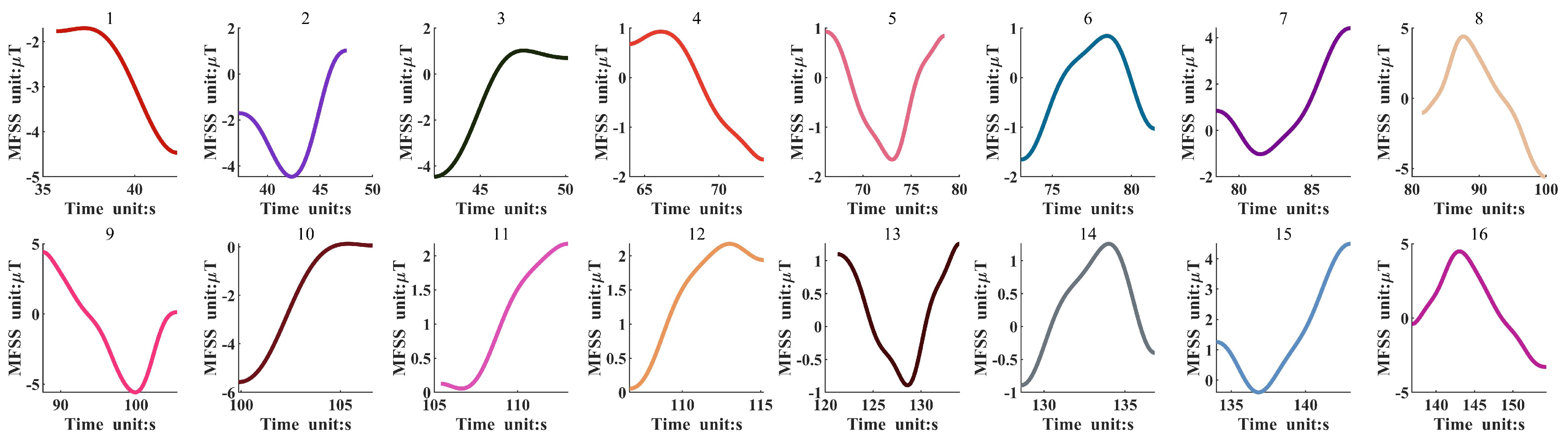
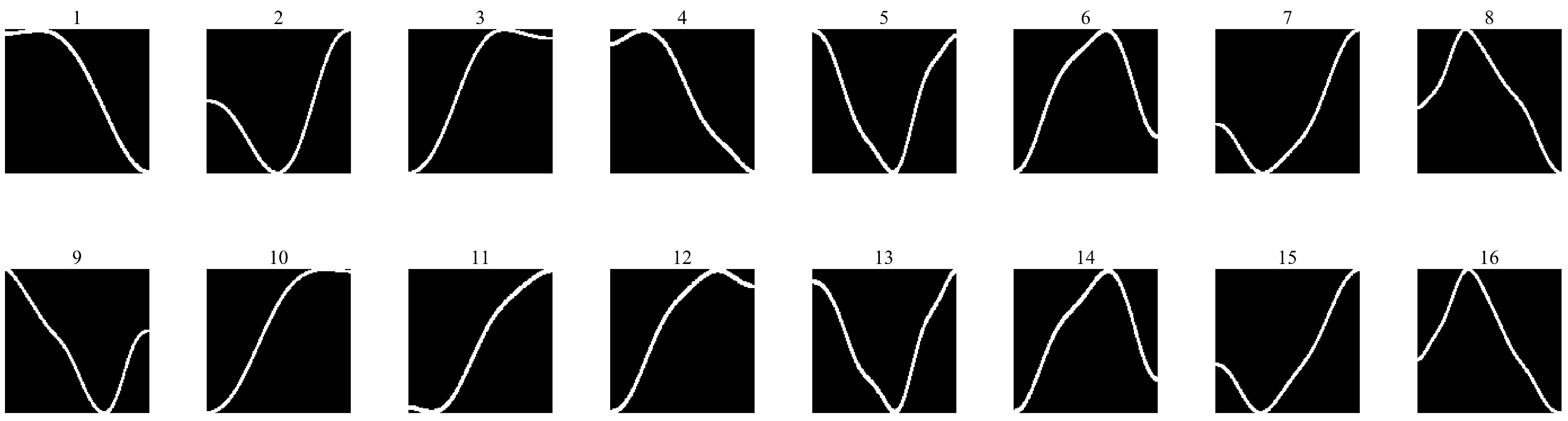
2.1. Construction of Magnetic Field Landmark Database

To save the cost of establishing the magnetic field landmark database, this paper dynamically collects magnetic field signals. After collecting the magnetic field signals, this paper adopts the Butterworth filter to eliminate the noise. When the tester holding the smartphone walks at a constant speed, the triaxial components of the magnetic field signal have obvious differences at the same position due to the pose change of the smartphone. So, this paper uses the modulus of the triaxial component of the magnetic field signal to build the database. The calculation formula for magnetic field signal modulus is as follows,

$$B_m=\sqrt{B_x^2+B_y^2+B_z^2}$$

(1)

where $B_m$ indicates the module of triaxial magnetic field signals and $B_x$, $B_y$, and $B_z$ indicate the x-, y-, and z-axis magnetic field signals. The accurate construction of the magnetic field landmark database is an important condition to ensure the accuracy of magnetic field matching and positioning. Magnetic field signal landmarks can be divided into intrinsic landmarks and organic landmarks based on whether they contain visible ferromagnetic substances. Among them, inherent landmarks refer to visible objects containing ferromagnetic material, including fixed structures in buildings such as elevators, escalators, stairs, water dispensers, iron doors, etc.; organic landmarks refer to non-visible objects containing ferromagnetic material. Although the specific structure of the landmark cannot be seen, the magnetic signal will produce long-term stable distortion features when passing through the landmark. The construction of a landmark database includes three steps, extracting magnetic field feature sequences, mapping magnetic field images, and expanding the magnetic field image database.

The specific steps for extracting magnetic field feature sequences are as follows, (1) detecting peaks and valleys in magnetic field signal sequences; (2) using the detected peaks/valleys as the starting point, detect the first point after/before the peak that starts to increase (or the first point after/before the valley that starts to decrease) from the left and right directions, respectively; (3) use the first increase/decrease point discovered on both sides as the window radius, and extend the window radius in the left and right directions from the starting point (peaks/valleys) to extract feature sequences; and (4) calculate the change rate of magnetic field signal intensity within the window and set a threshold. If the change rate exceeds the threshold, the sequence will be recorded as a landmark. Otherwise, return to (2) until the data traversal is completed.

The specific steps for magnetic field image mapping are as follows. (1) Interpolating the magnetic field signal sequence to increase sampling points to avoid sparse pixel points on the image; (2) subtract the minimum value from the magnetic field signal strength, and then multiply it by a scale parameter (in this paper, it is 100); (3) the difference between the maximum and minimum values of the magnetic field signal strength is mapped as columns of the image, and the sampling point index of the magnetic field signal are rows of the image, which are assigned one by one to complete the image mapping; and (4) annotate the position of the mapped image and store it as a landmark.

After mapping the magnetic field image, the changing trend of the magnetic field signal sequence can be extracted, which weakens the impact of different smartphones during the landmark detection process (different smartphones often have the same changing trend, but the overall magnetic field signal strength will have a deviation [8]). At the same time, converting magnetic field signals into images can effectively perform two-dimensional spatial calculations. Considering the mismatch in walking speed during data collection, using magnetic field signal images for detection may result in a decrease in accuracy. Therefore, this paper expands the database by stretching magnetic field images. This paper considers the differences in walking speed between different tests when setting the stretching factor. After empirical testing, the stretching factor is set to 0.5∼1.5.

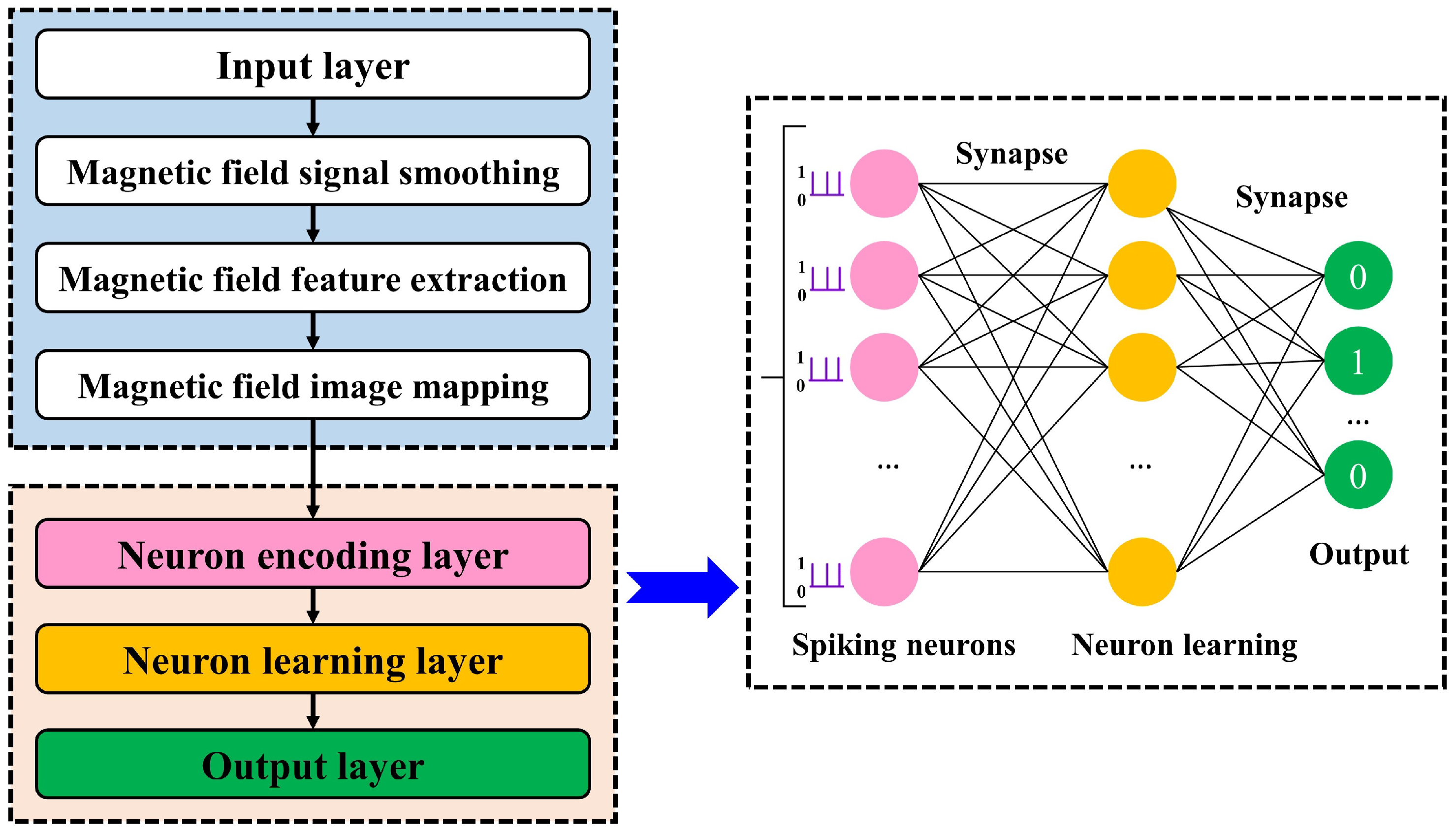
2.2. SNN Architecture

In this paper, SNN is used to learn and detect magnetic field landmarks. The SNN architecture is shown in Figure 2. After mapping the magnetic field image, we use the phase encoding method to convert the image into spike signals that conform to the characteristics of biological neurons and input them into SNN for model training. In the process of magnetic field landmark detection, the neural network module is directly called to output the position of the matching landmark.

2.2.1. Neuron Encoding Model

SNN simulates biological neurons receiving spike signal sequences as inputs. To design an efficient SNN architecture, it is necessary to adopt appropriate spike encoding methods to encode magnetic field images into spike signal sequences. This paper uses phase encoding to encode magnetic field images into spike signal sequences of neurons. The phase encoding formula is shown as

$$os{c}_i=A\cos (B·t+{\varphi }_i)$$

(2)

where A is the amplitude factor, B is the period factor, t is the current time of the spike, ${\varphi }_i$ represents the phase of the $i^{th}$ pixel, and it is calculated as follows

$${\varphi }_i={\varphi }_0+(i-1)\Delta {\varphi }_i$$

(3)

where ${\varphi }_0$ is the initial phase, and $\Delta {\varphi }_i$ is the phase difference between two adjacent pixel points, calculated as follows

$$\Delta {\varphi }_i\le \frac{2\pi }{N_{RF}}$$

(4)

where $N_{RF}$ represents the number of pixels in the time window.

2.2.2. Neuron Dynamics Model

The neuron dynamics model is the basic computing unit of the neural network. LIF is a typical neuron dynamics model. It can capture the key dynamics of the input and output characteristics of biological neural networks, so it has been widely used in neuron computing. In this paper, the LIF neuron dynamics model is used as the basic computing unit of the SNN. For the nervous system, the information transmission of neurons can be expressed as the transmission of membrane potential from presynaptic neurons to postsynaptic neurons. The membrane potential of a postsynaptic neuron is determined by the membrane potential of all presynaptic neurons connected to the neuron. The membrane potential of postsynaptic neurons is calculated as follows [14]

$$V\left(t\right)=\sum _{i=1}^{\eta }{w}_i\sum _{t_i<t}K(t-t_i)+V_{rest}$$

(5)

where $\eta$ is the number of input spike; i is the index of the input spike; t represents the current time; $t_i$ is the release time of the $i^{th}$ input spike; $w_i$ represents the weight of the $i^{th}$ input synapse; $V_{rest}$ is the resting potential of the current neuron; and $K(t-t_i)$ is the kernel function representing the delay effect. The specific calculation formula is as follows:

$$K(t-t_i)=V_0\left[\exp \left(-\frac{t-t_i}{\tau }\right)-\exp \left(-\frac{t-t_i}{{\tau }_s}\right)\right]$$

(6)

Among them, $\tau$ indicates the delay parameter of membrane integration current; ${\tau }_s$ is the delay parameter of synaptic current; and $V_0$ is the normalization factor.

$$V_0=\frac{\tau ·{\tau }_s}{\tau -{\tau }_s}\ln \frac{\tau }{{\tau }_s}$$

(7)

According to the (5) and (6), the membrane potential intensity changing trend can be described as that after the peak value is generated, the membrane potential intensity rises from $V_{rest}$ to $V_{th}$, and then gradually decays and tends to $V_{rest}$. When the potential of the neuron reaches $V_{th}$, the spike will be activated. However, the transmission of the spike is not only related to its release time but also related to the strength of the synaptic connection. When the synaptic weight $w_i$ is positive, the presynaptic potential has a long-term enhancement effect; when $w_i$ is negative, the presynaptic potential will produce a long-term inhibitory effect.

2.2.3. Neuron Learning Mechanism

The cost function of neurons in the learning process is defined as

$$E_{\pm }=\pm \left(V_{th}-V\left(t_{max}\right)\right)\Theta \left[\pm \left(V_{th}-V\left(t_{max}\right)\right)\right]$$

(8)

$$\Theta \left(x\right)=\left\{\begin{array}{c}\hfill 1, x\ge 0\\ \hfill 0, x<0\end{array}\right.$$

(9)

where $V_{th}$ is the spike release threshold and $t_{max}$ is the maximum release time. The derivative of the cost function over weight is:

$$-\frac{d{E}_{\pm }}{d{w}_i}=\pm \sum _{t_i<t_{max}}K(\Delta t_i)\pm \frac{\partial V\left(t_{max}\right)}{\partial t_{max}}\frac{d{t}_{max}}{d{w}_i}$$

(10)

The updated rules for synaptic transmission weights are as follows:

$$\Delta w_i=\left\{\begin{array}{c}\hfill \lambda \sum _{t_i<t_{max}}K(t_{max}-t_i)\\ \hfill -\lambda \sum _{t_i<t_{max}}K(t_{max}-t_i)\end{array}\right.$$

(11)

Among them, parameters $\lambda$ represent the learning rate and describe the magnitude of synaptic weight adjustment.

3. Ranging Based on DTMB Signals

DTMB is a Chinese standard [25], and together with the Advanced Television System Committee (ATSC) of the United States and the Digital Video Broadcasting (DVB) of Europe become the main digital broadcasting system. In this paper, the DTMB signals are used for ranging estimation.

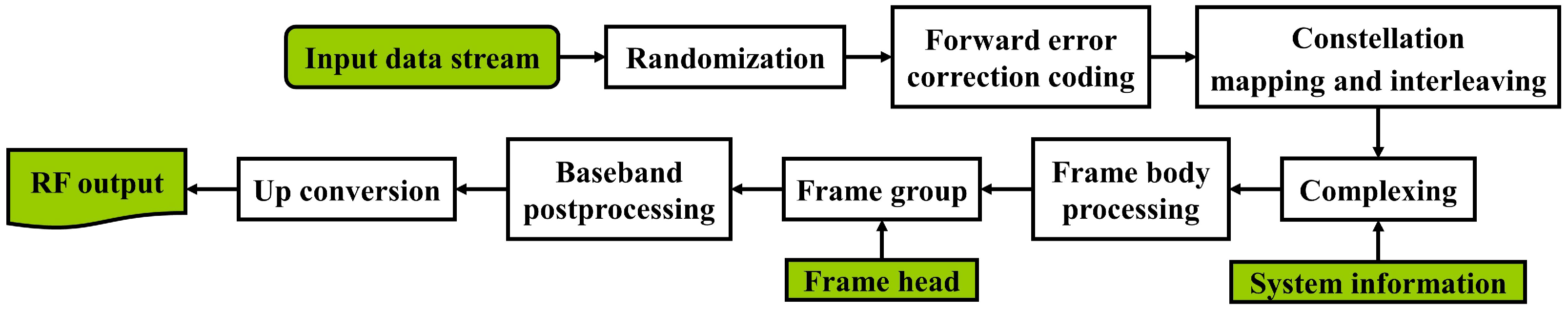
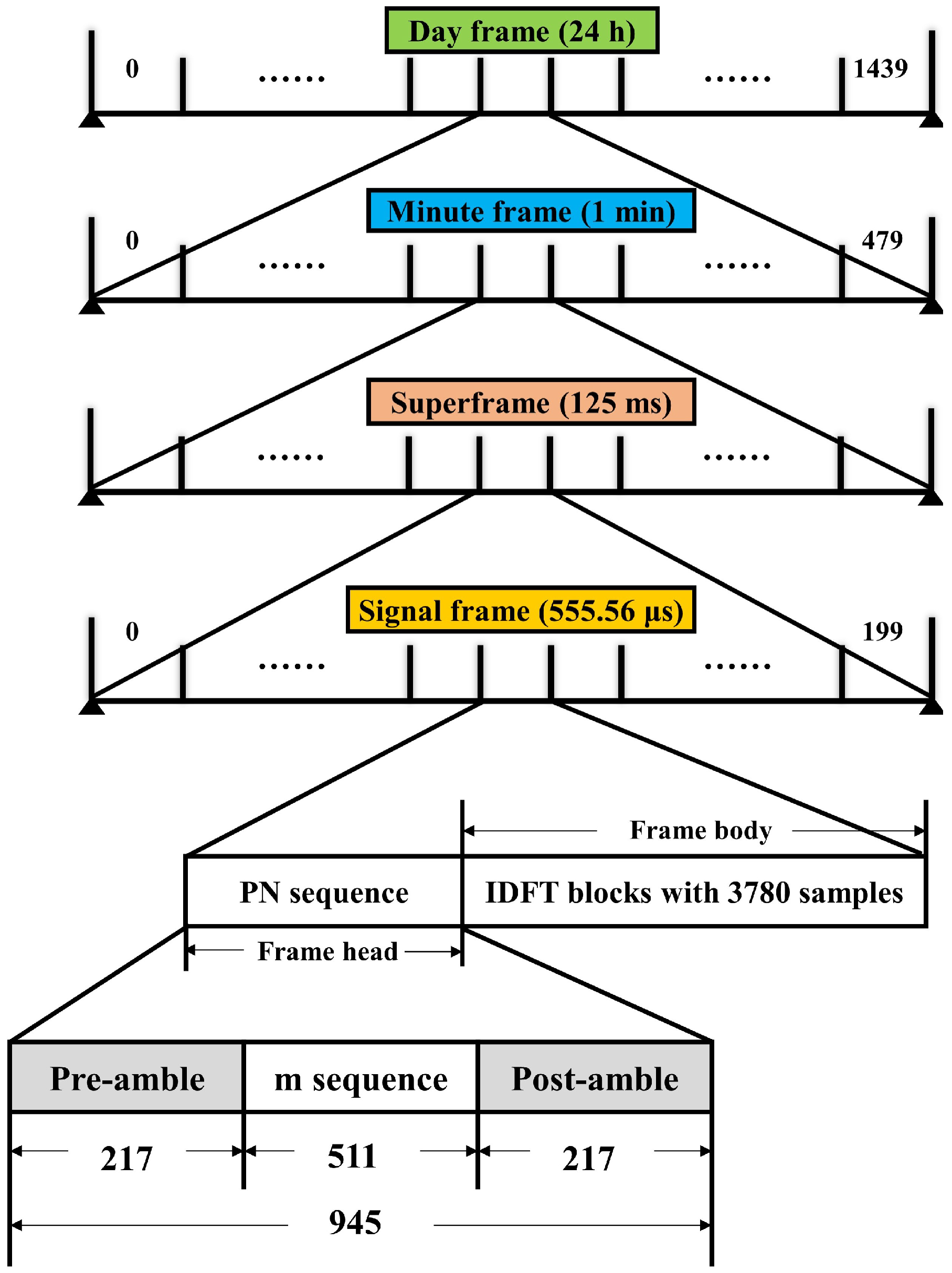
3.1. DTMB System Description

The DTMB system uses OFDM modulation to achieve robust transmission in multipath scenarios. The DTMB system supports single-carrier and multi-carrier modulation. This study focuses on multi-carrier modulation. The DTMB signals are transmitted in streams and organized in frames. The DTMB transmitting system completes the conversion from the input data stream to the DTMB channel transmission signal, and the transmitting principle of the DTMB system is shown in Figure 3. The input data stream is encoded by scrambler (randomization), forward error correction coding, constellation mapping from bitstream to symbol stream, and interweaved to form a data block. After the data block and system information are multiplexed, the frame body is formed by frame body data processing. The frame body and the corresponding frame head (PN sequence) are multiplexed into a signal frame and converted into a baseband output signal with bandwidth within 8 MHz after baseband post-processing. Finally, the signal is converted into an RF signal (UHF and VHF) by orthogonal upconversion.

The frame structure of the DTMB system is shown in Figure 4, which is a four-layer structure. The basic unit of the frame structure is the signal frame, which is composed of the frame head and the frame body. The frame head is a PN sequence with a preamble and a postamble. The PN sequence includes three different length modes, 420, 595, and 945, at the sampling rate of 7.56 MHz. In our study, the length mode of the PN sequence is 945. The frame body is an Inverse Discrete Fourier Transform (IDFT) block with 3780 subcarriers, 36 of which are used to transmit Transmission Parameter Signaling (TPS) to provide demodulation and to decode information at the receiver. The superframe consists of 200 signal frames. In a superframe, each PN sequence is different from the other 199, but it is repeated in every superframe. The minute frame is defined as 480 superframes that last 1 min. The top layer of the frame structure is called the calendar day frame, starting from 00:00:00 and ending at 24:00:00. The signal structure is periodic and keeps synchronization with natural time.

3.2. Ranging Estimation

The DTMB signal system adopts Time-Domain Synchronous Orthogonal Frequency Division Multiplexing (TDS-OFDM) mode. Assuming $X\left(k\right)$ represents the $k^{th}$ subcarrier in the OFDM system, and $k=0,...,N-1$. Then, the transmitted $l^{th}$ OFDM sample is described as [26]:

$$x\left(l\right)=\frac{1}{\sqrt{N}}\sum _{k=0}^{N-1}X(k)e^{j2\pi kl/N},l=0,\dots N-1.$$

(12)

After the Fast Fourier Transform (FFT), the $k^{th}$ subcarrier of the $m^{th}$ signal frame received in the frequency domain is expressed as [27]:

$$\begin{array}{c}\hfill \begin{array}{cc}\hfill Y_m\left(k\right)& =e^{j\frac{2\pi }{N}\left(m{N}_s+N_g\right)\left[k\alpha +ϵ(1+\alpha )\right]}{A}_N(k\alpha +ϵ(1+\alpha ))\hfill \\ \hfill & ·X_m\left(k\right)C\left(k\right)+I_m\left(k\right)+w_m\left(k\right)\hfill \end{array}\end{array}$$

(13)

where $N_s$ is the total sample of a signal frame, $N_g$ is the length of the guard interval, $\alpha \triangleq \Delta T/T$ is the normalized Sampling Frequency Offset (SFO), T is the sampling period, $ϵ\triangleq \Delta fNT$ is the normalized Carrier Frequency Offset (CFO), $C\left(k\right)$ is the channel frequency response, $w_m\left(k\right)\sim N(0,{\sigma }^2)$ is the Gaussian noise, $A_N\left(k\right)$ is the attenuation factor

$$\begin{array}{c}\hfill \begin{array}{c}\hfill A_N\left(x\right)\triangleq \frac{1}{N}\sum _{i=0}^{N-1}{e}^{j\frac{2\pi }{N}ix}=e^{j\pi x(N-1)/N}\frac{\sin \left(\pi x\right)}{N\sin (\pi x/N)}\end{array}\end{array}$$

(14)

and $I_m\left(k\right)$ represents the Inter-Carrier Interference (ICI):

$$\begin{array}{c}\hfill \begin{array}{cc}\hfill I_m\left(k\right)& =\sum _{i=0,i\ne k}^{N-1}{e}^{j\frac{2\pi }{N}\left(m{N}_s+N_g\right)\left[i\alpha +ϵ(1+\alpha )\right]}\hfill \\ \hfill & ·A_N(i\alpha +ϵ(1+\alpha )+i-k)X_m\left(i\right)C\left(i\right)\hfill \end{array}\end{array}$$

(15)

The data modulated on the TPS can remain unchanged for a long time, such as for dozens of days. Consequently, the CFO of the $m^{th}$ signal frame $\Delta f_m$ can be obtained as [24]:

$$\begin{array}{c}\hfill \Delta f_m=-\frac{\angle \left[{\displaystyle \sum _{k\in K_{TPS}}}{Y}_{m+1}^{\ast }\left(k\right)Y_m\left(k\right)\right]}{2\pi N_{s}T}\end{array}$$

(16)

The CFO is mainly caused by oscillator mismatch between the transmitter and receiver and the Doppler effect. It can be defined as

$$\Delta f_m=f_m^d+f_m^s+q_m$$

(17)

where $f_m^d$ is caused by the Doppler effect, $f_m^s$ is caused by oscillator mismatch between receiver and transmitter, and $q_m$ is the Gaussian noise. Generally, $f_m^s$ is stable, so suppose it remains unchanged during a test. Thus, the $f_m^s$ can be obtained by holding still for a few seconds after the test starts. The Doppler speed $\Delta v_{m+1,m}^{\mathrm{dtmb}}$ between the ${(m+1)}^{th}$ signal frame to the transmitter and the $m^{th}$ signal frame to the transmitter is expressed as [28]

$$\begin{array}{c}\hfill \begin{array}{c}\hfill \Delta v_{m+1,m}^{\mathrm{dtmb}}=\left(\Delta f_m-f_m^s\right)·\frac{c}{f_c}\end{array}T\end{array}$$

(18)

where c is the light speed and $f_c$ is the carrier frequency. Finally, the range difference $\Delta r_m^{\mathrm{dtmb}}$ between the $m^{th}$ signal frame to the transmitter and the first signal frame to the transmitter is expressed as:

$$\Delta r_m^{\mathrm{dtmb}}=\sum _{i=0}^{m-1}\Delta v_{i+1,i}^{\mathrm{dtmb}}{N}_{s}T$$

(19)

4. Hybrid PDR Integrating Magnetic Field Signals and DTMB Signals

Magnetic field landmarks cannot provide unique detection results, because similar magnetic field features can be found in different places. To eliminate magnetic field landmarks with significant anomalies, this paper proposes an optimal landmark selection method based on DTMB ranging information, and then the optimal landmarks are used for fusion positioning.

4.1. Optimal Landmark Selection

Assume that ${\mathit{P}}^{\mathrm{mag}}=\left\{{\mathit{P}}_1^{\mathrm{mag}},{\mathit{P}}_2^{\mathrm{mag}},\dots ,{\mathit{P}}_n^{\mathrm{mag}}\right\}$ is the position coordinates of the candidate landmarks obtained based on magnetic field signal matching, where n represents the number of landmarks. Then, compare the distance between the candidate magnetic field landmark and the DTMB base station with the DTMB signal ranging results, and then select the landmarks with a difference less than the threshold parameter as the optimal landmarks. The calculation formula for the optimal landmark ${\tilde{\mathit{P}}}^{\mathrm{mag}}$ is as follows

$${\tilde{\mathit{P}}}^{\mathrm{mag}}=\left|\parallel {\mathit{P}}_i^{\mathrm{mag}}-{\mathit{P}}^{\mathrm{base}}\parallel -\Delta r^{\mathrm{dtmb}}\right|<{\delta }^r,i=1,2,\dots ,n.$$

(20)

where ${\delta }^r$ is a distance difference threshold, ${\mathit{P}}^{\mathrm{base}}$ is the position coordinate of the DTMB base station, and $\Delta r^{\mathrm{dtmb}}$ is the ranging result from DTMB signals.

4.2. Hybrid Positioning Model

In this paper, we use the Attitude and Heading Reference System (AHRS) [29,30] to obtain the raw PDR trajectory. To achieve robust PDR, we use the position information from the optimal landmark and the ranging information from the single base station DTMB signals as the observation, and then use the EKF to achieve the fusion positioning. The state model of the fusion framework in this paper is defined as:

$${\mathit{X}}_t={\mathit{F}}_{t-1}{\mathit{X}}_{t-1}+{\mathit{w}}_t$$

(21)

The state vector is defined as:

$${\mathit{X}}_t={\left[x,y,\dot{\theta },\theta ,v\right]}_t^T$$

(22)

where t represents the current time, x is the position of the eastern direction, y is the position of the northern direction, $\dot{\theta }$ is the heading change, $\theta$ is the heading, and v is the motion velocity. The state equation is defined as follows

$$\left\{\begin{array}{cc}\hfill x_t& =x_{t-1}+v_{t-1}·\Delta t·cos{\theta }_{t-1}+w_1\hfill \\ \hfill y_t& =y_{t-1}+v_{t-1}·\Delta t·sin{\theta }_{t-1}+w_2\hfill \\ \hfill {\dot{\theta }}_t& ={\dot{\theta }}_{t-1}+w_3\hfill \\ \hfill {\theta }_t& ={\theta }_{t-1}+\Delta t·{\dot{\theta }}_{t-1}+w_4\hfill \\ \hfill v_t& =v_{t-1}+w_5\hfill \end{array}\right.$$

(23)

where $\Delta t$ is the time interval between the time $t-1$ and t, ${\mathit{w}}_t={\left\{w_1,w_2,...,w_5\right\}}_t$ is the noise vector of the state equation. The state transition matrix ${\mathit{F}}_t$ is written as:

$${\mathit{F}}_t=\left[\begin{array}{ccccc}1& 0& 0& 0& \Delta t·cos{\theta }_{t-1}\\ 0& 1& 0& 0& \Delta t·sin{\theta }_{t-1}\\ 0& 0& 1& 0& 0\\ 0& 0& \Delta t& 1& 0\\ 0& 0& 0& 0& 1\end{array}\right]$$

(24)

The process noise matrix ${\mathit{W}}_t$ [24,31] is expressed as

$${\mathit{W}}_t={\left[\begin{array}{ccccc}{w}_1\Delta t+\frac{w_5{a}^2\Delta t^3}{3}& \frac{w_{5}ab\Delta t^3}{3}& 0& 0& \frac{w_{5}a\Delta t^2}{2}\\ \frac{w_{5}ab\Delta t^3}{3}& w_2\Delta t+\frac{w_5{b}^2\Delta t^3}{3}& 0& 0& \frac{w_{5}a\Delta t^2}{2}\\ 0& 0& w_3\Delta t^2& \frac{w_3\Delta t^3}{2}& 0\\ 0& 0& \frac{w_3\Delta t^3}{2}& \frac{w_3\Delta t^4}{4}& 0\\ \frac{w_{5}a\Delta t^2}{2}& \frac{w_{5}a\Delta t^2}{2}& 0& 0& w_5\end{array}\right]}_t$$

(25)

where $a=cos{\theta }_{t-1}$ and $b=sin{\theta }_{t-1}$. The observation vector ${\mathit{Z}}_t$ is defined as:

$${\mathit{Z}}_t={\left[x^{\mathrm{mag}},y^{\mathrm{mag}},\Delta r^{\mathrm{dtmb}},{\theta }^{\mathrm{pdr}},v^{\mathrm{pdr}}\right]}_t^T$$

(26)

Among them, $x^{\mathrm{mag}}$ and $y^{\mathrm{mag}}$ are the positions from optimal magnetic field landmark, which is detailed in Section 2 and Section 4.1. $\Delta r^{\mathrm{dtmb}}$ is from the DTMB signals, which is detailed in Section 3. The heading ${\theta }^{\mathrm{pdr}}$ and speed $v^{\mathrm{pdr}}$ are estimated by AHRS based on Micro-Electro-Mechanical Systems (MEMS) sensors. The observation model is defined as:

$${\mathit{Z}}_t={\mathit{H}}_t{\mathit{X}}_t+{\mathit{\delta }}_t$$

(27)

The observation equation can be expressed as:

$$\left\{\begin{array}{c}{x}_t^{\mathrm{mag}}=x_t+{\delta }_1\hfill \\ y_t^{\mathrm{mag}}=y_t+{\delta }_2\hfill \\ \Delta r_t^{\mathrm{dtmb}}=r_t-r_{t-1}+{\delta }_3\hfill \\ {\theta }_t^{\mathrm{pdr}}={\theta }_t+{\delta }_4\hfill \\ v_t^{\mathrm{pdr}}=v_t+{\delta }_5\hfill \end{array}\right.$$

(28)

The $r_t$ represents the range from the pedestrian to the DTMB transmitter and it is expressed as

$$r_t=\sqrt{{\left(x_t-x_{\mathrm{base}}\right)}^2+{\left(y_t-y_{\mathrm{base}}\right)}^2+{\left(z_t-z_{\mathrm{base}}\right)}^2}$$

(29)

where $x_{\mathrm{base}}$, $y_{\mathrm{base}}$, and $z_{\mathrm{base}}$ are the position coordinates of the DTMB signal transmitter, respectively; $z_{\mathrm{t}}$ is the height of the pedestrian movement plane, which is set to 0. The observation Jacobian matrix ${\mathit{H}}_t$ is shown as:

$${\mathit{H}}_t=\left[\begin{array}{ccccc}1& 0& 0& 0& 0\\ 0& 1& 0& 0& 0\\ {\displaystyle \frac{x_t-x_{\mathrm{base}}}{r_t}}& {\displaystyle \frac{y_t-y_{\mathrm{base}}}{r_t}}& 0& 0& 0\\ 0& 0& 0& 1& 0\\ 0& 0& 0& 0& 1\end{array}\right]$$

(30)

The observation noise is ${\mathit{\delta }}_t\sim N\left(0,{\mathit{R}}_t\right)$ and the observation covariance matrix ${\mathit{R}}_t$ is:

$${\mathit{R}}_t={\left[{\sigma }_{x^{\mathrm{mag}}}^2,{\sigma }_{y^{\mathrm{mag}}}^2,{\sigma }_{\Delta r^{\mathrm{dtmb}}}^2,{\sigma }_{{\theta }^{\mathrm{pdr}}}^2,{\sigma }_{v^{\mathrm{pdr}}}^2\right]}_t$$

(31)

5. Tests and Results

To validate the proposed method, we conducted field tests in both indoor and outdoor environments. Among them, there is no DTMB information for indoor testing, mainly testing the feasibility of magnetic field landmarks.

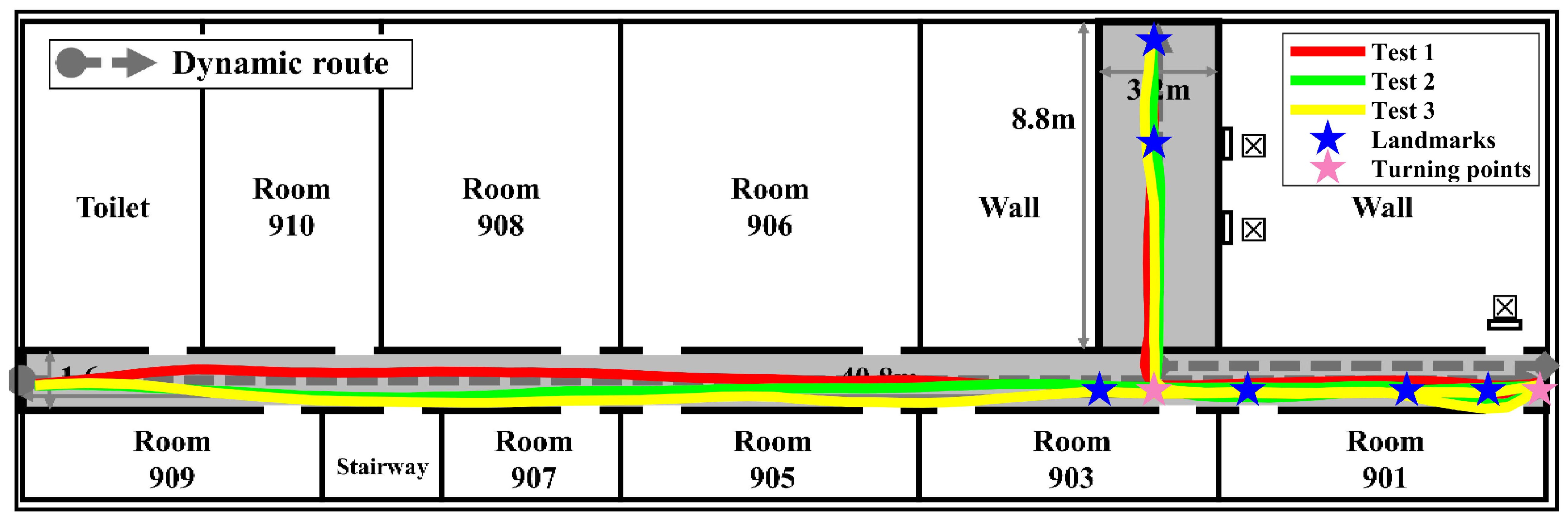
5.1. Indoor Tests

We collected indoor test data at the Xinghu Building of Wuhan University. The floor map of the indoor data collection scenario is shown in Figure 5. The collected mobile device is the Huawei P30. To achieve mutual verification of multiple sets of tests, the testers walked along the testing route three times.

After data collection is completed, the magnetic field sequence signals of the three tests are smoothed and feature sequences are extracted to obtain a landmark database for each group of tests. The original magnetic field signals and smooth magnetic field signals of the three tests are shown in Figure 6. It can be seen that the magnetic field signals of the three tests have the same change trend. However, the magnetic field signal curves have a deviation due to the different motion speeds.

Using the smoothed triaxial modulus for indoor landmark feature extraction, the extraction results are shown in Figure 7. Among them, nine landmarks were extracted in test 1, and eight features were extracted in test 2 and test 3. The results of image mapping from landmark feature curves are shown in Figure 8, which shows that the curve features of the magnetic field signals are well preserved in the form of images. To adapt to the SNN structure, the magnetic field image is converted into a spike sequence, as shown in Figure 9.

We use three tests for mutual verification to test the accuracy of landmark detection. During testing, one of the tests is used as the test set, and the other two tests are used as the magnetic field landmark database for SNN model matching. Then, the intersection of the matching results is extracted as the final result of this test. To verify the performance of SNN, we use the DTW [32] method as a comparative test. The matching results for each test set of the two methods are shown in Figure 10. Among them, Figure 10a shows the results of the DTW method, and it can be seen that a total of nine landmark intersections were matched in test 1, while eight landmark intersections were matched in both test 2 and test 3. Figure 10b shows the results of the SNN method, and it can be seen that a total of seven landmark intersections were matched in test 1, while six landmark intersections were matched in both test 2 and test 3. Comparing the matching results of the two methods, it can be concluded that SNN matching results are more accurate than DTW overmatching. This is important for magnetic field matching, as similar magnetic field sequences are often in different positions. Overmatching will lead to landmark recognition errors and significant position deviations. After further selection, we selected six intersection landmarks from three tests based on the matching results of the SNN method, as the final landmarks. Meanwhile, we also extracted the turning points of the motion trajectory and used them as the calibration points for the final PDR trajectory, along with the magnetic field landmarks. The PDR trajectory calibration results are shown in Figure 11. It can be seen that after landmark calibration, the PDR trajectories of the three tests can almost overlap, which is in line with the actual motion state.

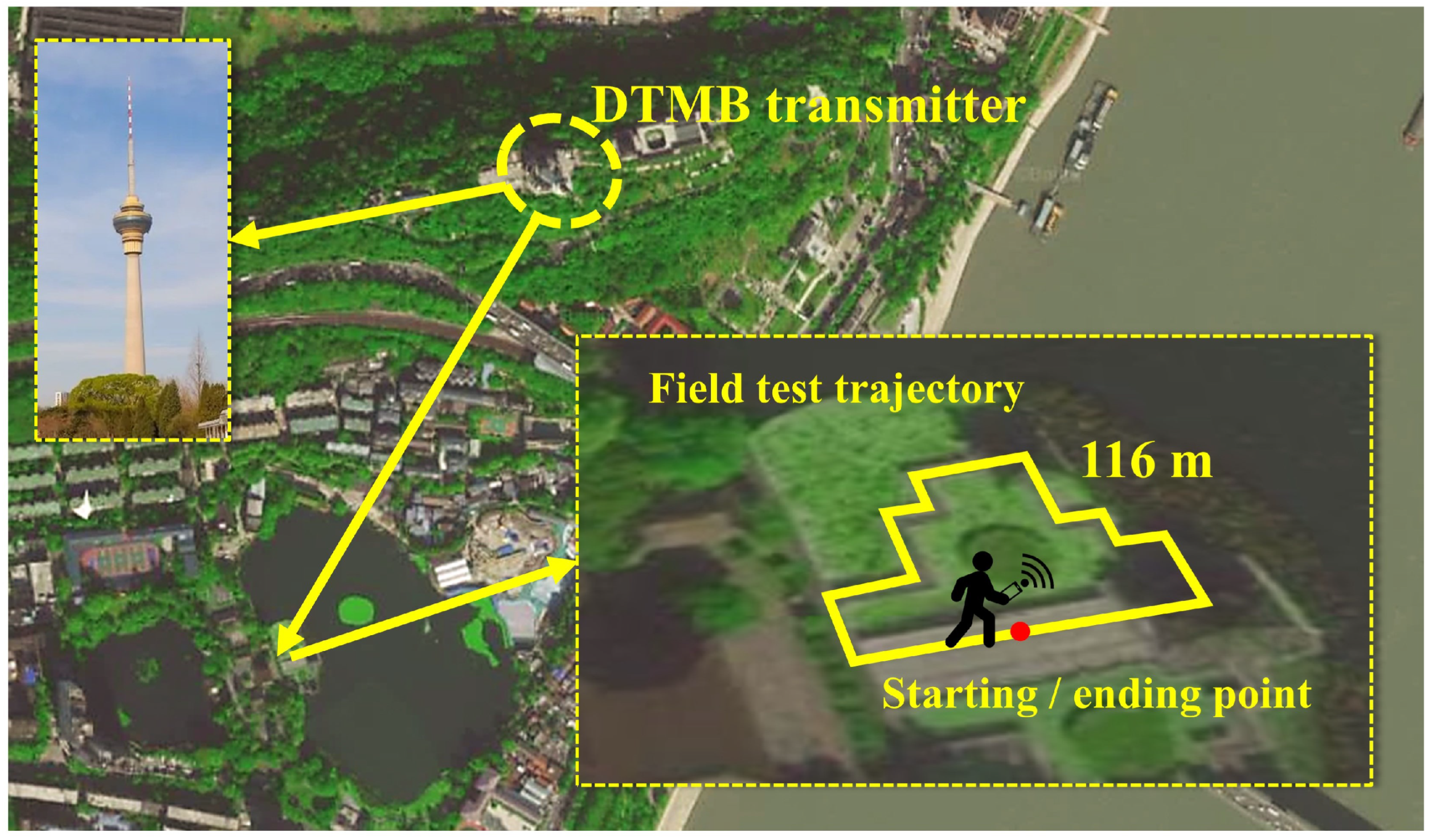
5.2. Outdoor Tests

We organized a real-world outdoor test to verify the proposed method. The test address is located in Lianhua Lake Park, Wuhan, China. During the test, the tester followed the planned route from the starting point to the endpoint, then returned to the starting point, walking for two laps. The trajectory is about 116 × 2 m, or 232 m. Figure 12 is a top view of the remote sensing of the real-world outdoor test.

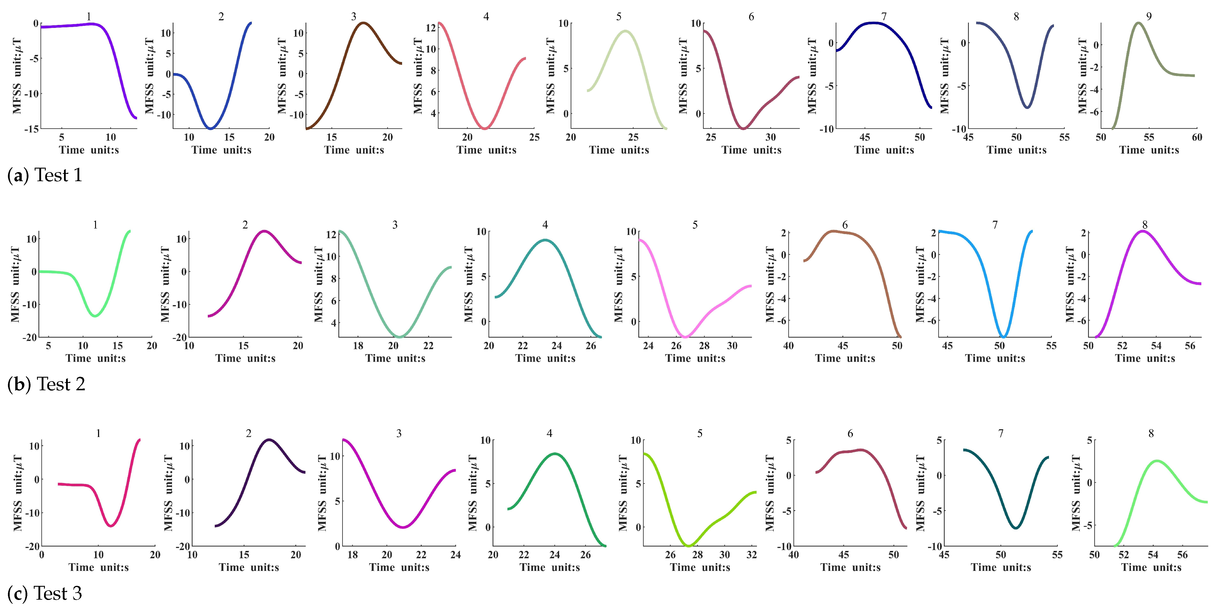
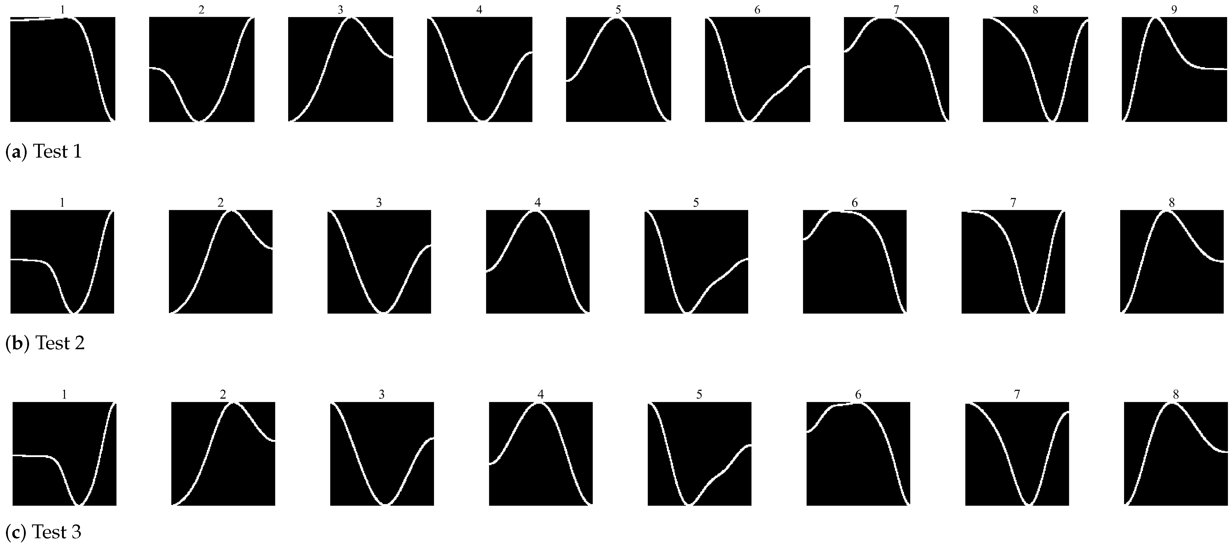
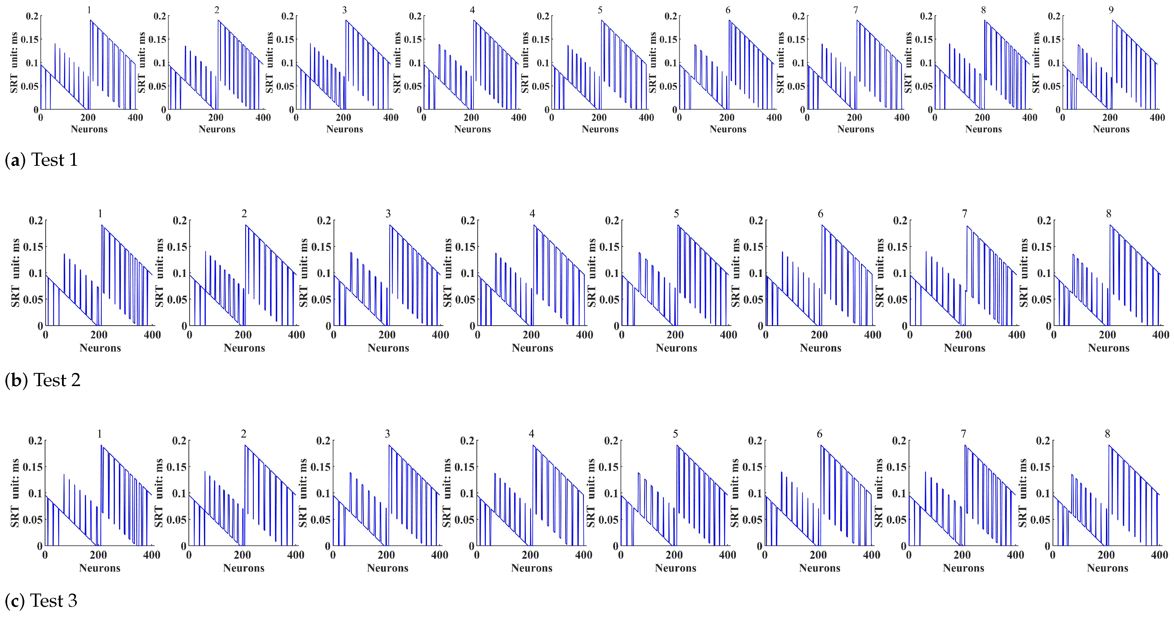
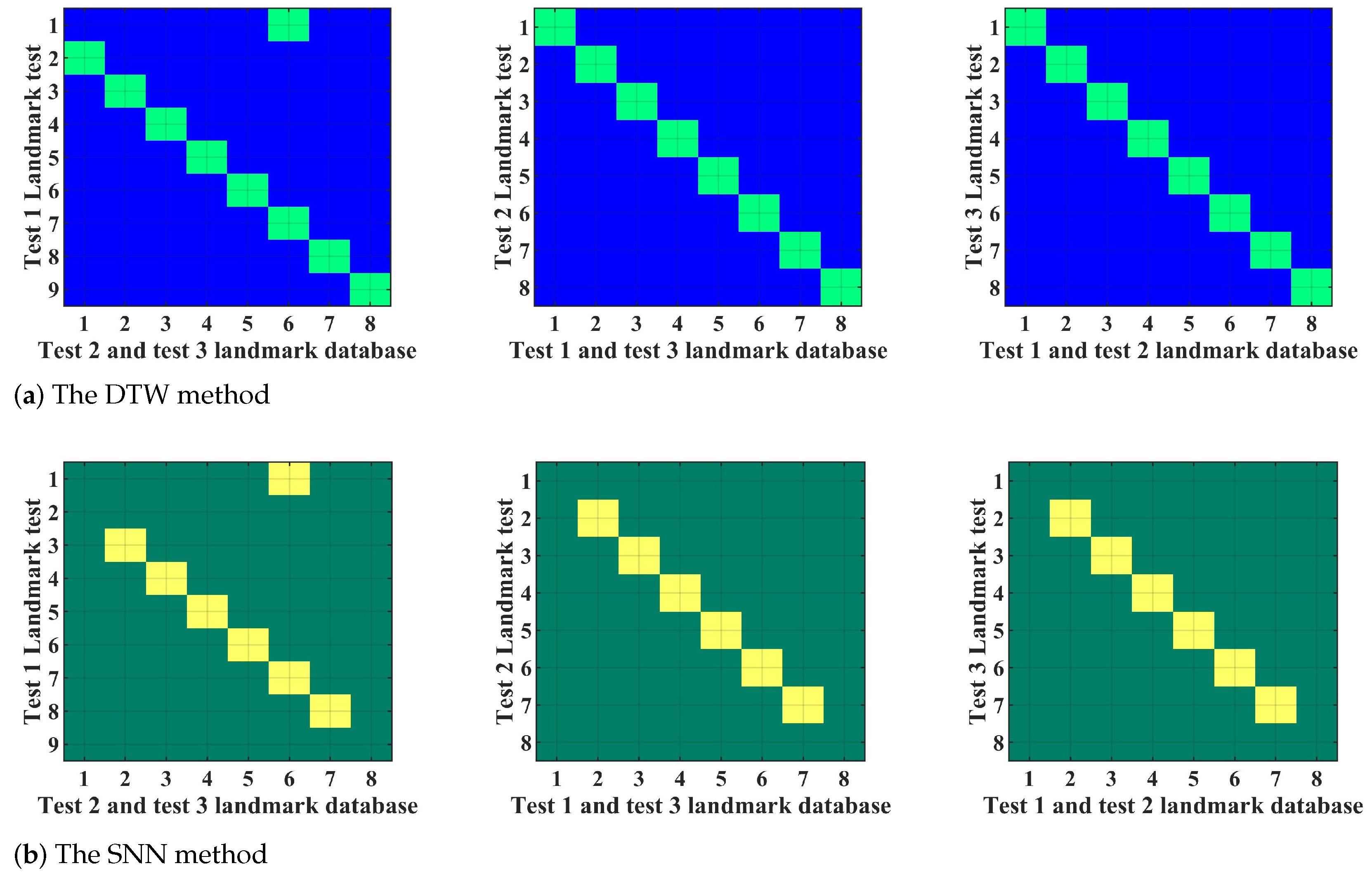
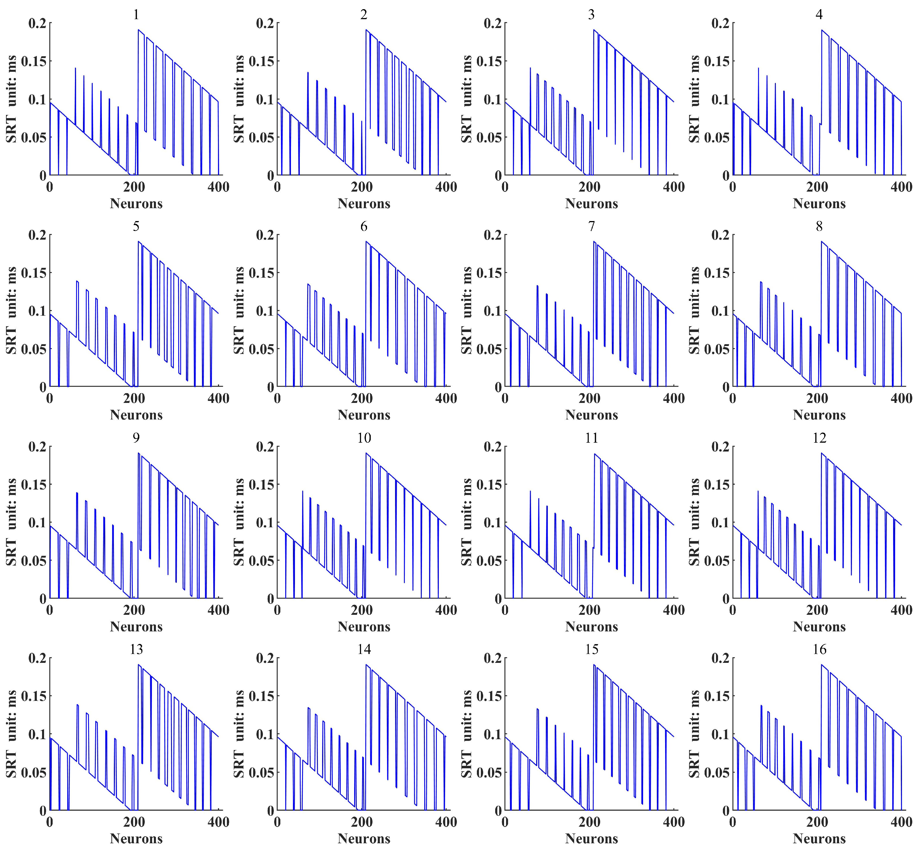
5.2.1. The Magnetic Field Landmark Detection Results

The original magnetic field signals and the smoothed magnetic field signals of the outdoor collected route are shown in Figure 13. Using the smoothed triaxial modulus for landmark feature extraction, the extraction results are shown in Figure 14, where numbers 1–8 represent the landmark features detected in the first lap and numbers 9–16 represent the landmark features detected in the second lap. The results of image mapping from landmark feature curves are shown in Figure 15, which shows that the curve features of the magnetic field signals are well preserved in the form of images.

To adapt to the SNN structure, the magnetic field image is converted into a spike sequence, as shown in Figure 16. We use the landmarks in the first lap as the database to train the SNN model, and then perform matching tests on the landmarks in the second lap. The matching results are shown in Figure 17, indicating that five magnetic field landmarks have been matched.

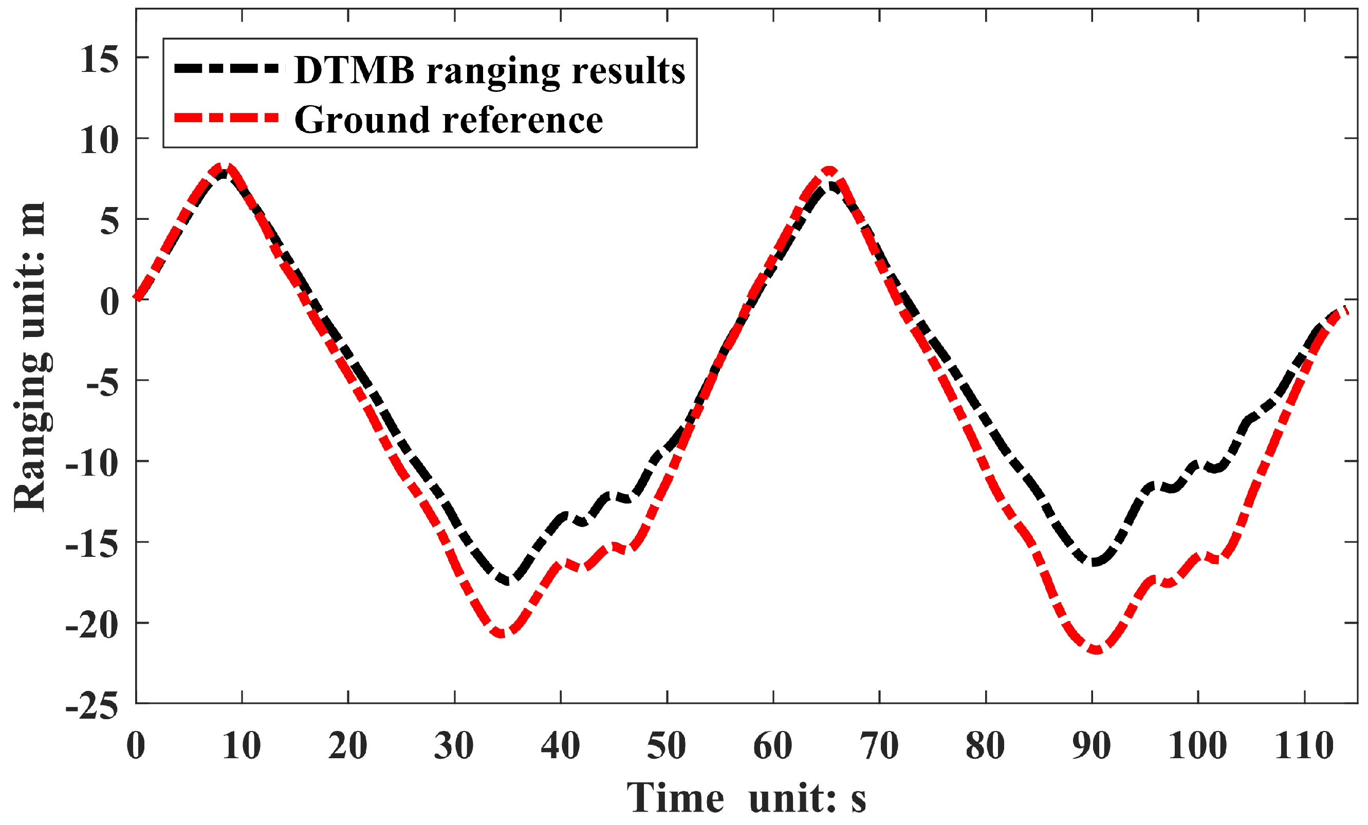
5.2.2. The Ranging Results from DTMB Signals

The ranging results based on DTMB signals are shown in Figure 18. In this paper, the ground position reference is first obtained through U-blox-M8U, and then obtained through RTK processing using data from the Wuhan IGS station (jfng) as the reference station. The distances from the ground position reference to the DTMB signal transmitter are calculated as a ranging reference, and then the ranging errors of the DTMB signal are counted. After statistics, the median error of DTMB ranging is 1.79 m and the maximum error is 5.92 m.

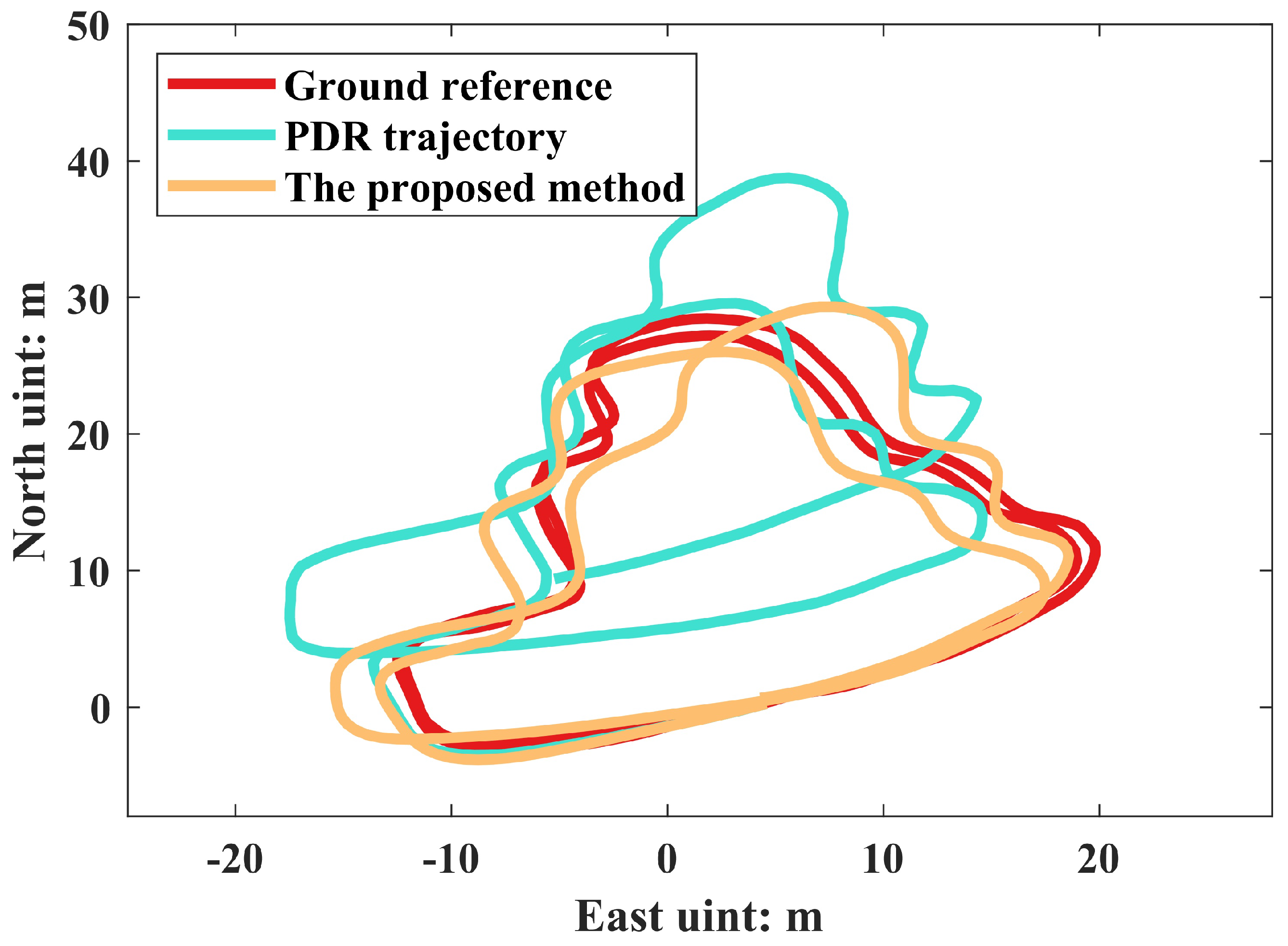
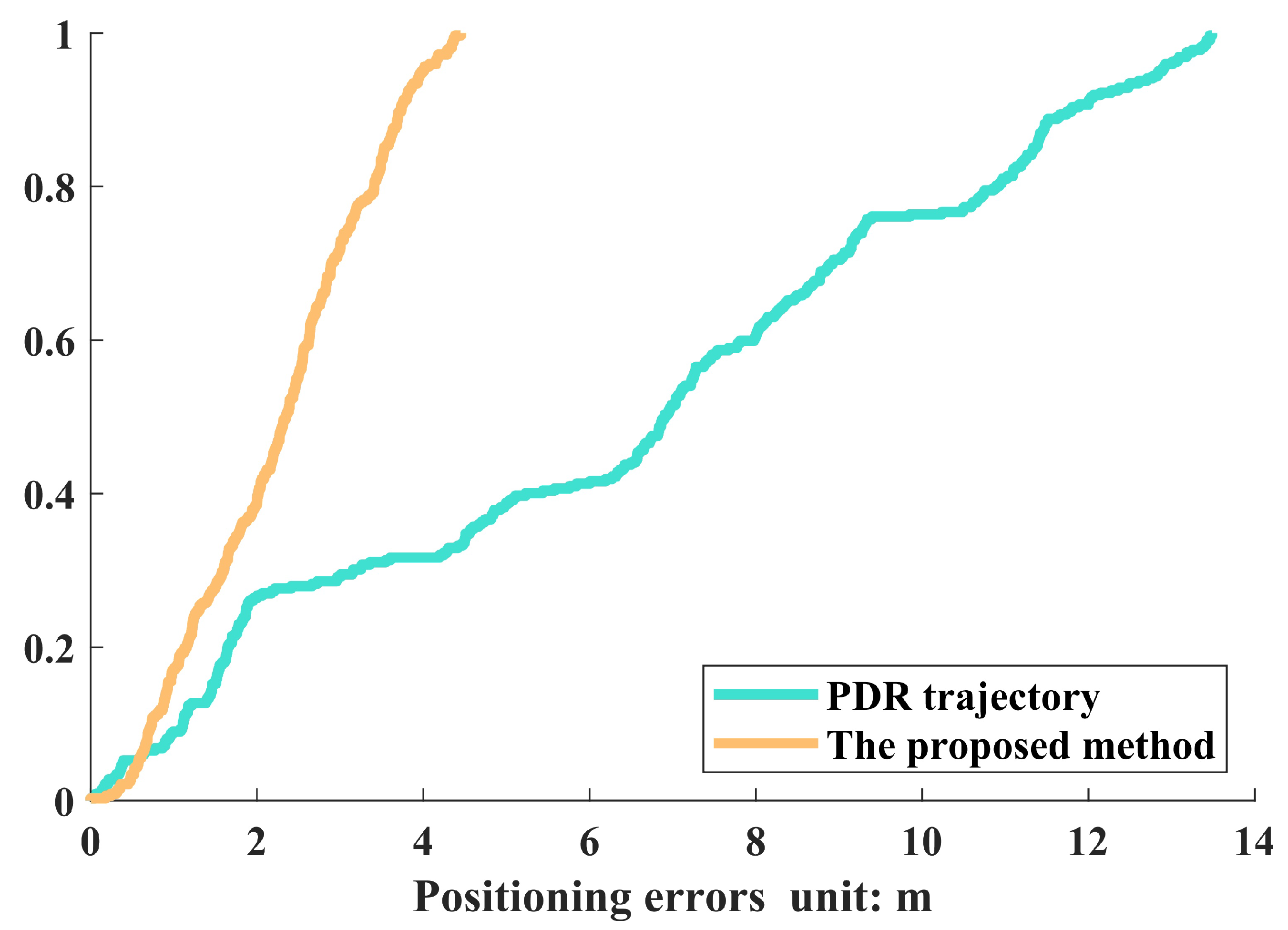
5.2.3. The Fusing Positioning Results

The outdoor field test results for the three positioning systems are shown in Figure 19, including ground reference, PDR, and the proposed method. It can be seen from Figure 19 that the trajectory direction calculated by the PDR deviates significantly compared to the ground reference, especially for the second lap of trajectory, where the heading of the PDR drifted severely. This is mainly due to the unstable attitude of the smartphone during the test. It is worth noting that after the fusion of the magnetic field landmarks and the ranging results from DTMB signals, the proposed method greatly corrects the PDR positioning trajectory.

The cumulative distribution function (CDF) of the PDR and the proposed method are shown in Figure 20. The CDF results suggest that the 68% positioning errors of PDR and the proposed method are 8.77 m and 2.84 m, and the 95% positioning errors are 12.84 m and 3.98 m, respectively. These statistical data indicate that the proposed method has superior positioning accuracy compared to PDR. Outdoor field testing has verified the positioning effectiveness of the proposed method.

6. Conclusions

Magnetic field signals are stable and ubiquitous, and DTMB signals have strong penetration and stable transmission over a large range. To improve the positioning performance of PDR, this paper proposes a robust PDR integrating magnetic field signals and DTMB signals. Inspired by that magnetic field signals can be mapped into images, this paper innovative converts magnetic field sequence signals into images, and first uses SNN to learn the magnetic field landmark images of the environment, and then uses a learning SNN model for magnetic field landmark detection. Meanwhile, the DTMB signals are collected by the self-developed signal receiver, and the ranging estimation based on the DTMB signals is achieved. Then, magnetic field landmarks were optimized based on the DTMB ranging information to eliminate the interference of similar magnetic field landmarks in positioning. Finally, EKF is used to fuse the position information from the optimal magnetic field landmarks and the ranging information from DTMB signals. The proposed method has been validated to be effective in both indoor and outdoor environments with positioning accuracy at the meter level. It will provide an alternative solution for seamless indoor and outdoor positioning. In future work, we will explore the indoor fusion positioning based on DTMB signals and integration positioning with other signals, such as WiFi, UWB, LTE, 5G, and audio.

References

- Li, Y.; Mi, J.; Xu, Y.; Li, B.; Jiang, D.; Liu, W. A robust adaptive filtering algorithm for GNSS single-frequency RTK of smartphone. Remote Sens. 2022, 14, 6388. [Google Scholar] [CrossRef]
- Feng, X.; Nguyen, K.A.; Luo, Z. WiFi access points line-of-sight detection for indoor positioning using the signal round trip Time. Remote Sens. 2022, 14, 6052. [Google Scholar] [CrossRef]
- Yu, Z.; Chaczko, Z.; Shi, J. A novel algorithm modelling for UWB localization accuracy in remote sensing. Remote Sens. 2022, 14, 4902. [Google Scholar] [CrossRef]
- Liu, Z.; Chen, L.; Zhou, X.; Shen, N.; Chen, R. Multipath tracking with LTE signals for accurate TOA estimation in the application of indoor positioning. Geo-Spat. Inf. Sci. 2023, 26, 31–43. [Google Scholar] [CrossRef]
- Ruan, Y.; Chen, L.; Zhou, X.; Liu, Z.; Liu, X.; Guo, G.; Chen, R. iPos-5G: Indoor positioning via commercial 5G NR CSI. IEEE Internet Things J. 2022, 10, 8718–8733. [Google Scholar] [CrossRef]
- Cao, S.; Chen, X.; Zhang, X.; Chen, X. Effective audio signal arrival time detection algorithm for realization of robust acoustic indoor positioning. IEEE Trans. Instrum. Meas. 2020, 69, 7341–7352. [Google Scholar] [CrossRef]
- Harle, R. A survey of indoor inertial positioning systems for pedestrians. IEEE Commun. Surv. Tutor. 2013, 15, 1281–1293. [Google Scholar] [CrossRef]
- Ashraf, I.; Zikria, Y.B.; Hur, S.; Park, Y. A comprehensive analysis of magnetic field based indoor positioning with smartphones: Opportunities, challenges and practical limitations. IEEE Access 2020, 8, 228548–228571. [Google Scholar] [CrossRef]
- Kuang, J.; Li, T.; Niu, X. Magnetometer bias insensitive magnetic field matching based on pedestrian dead reckoning for smartphone indoor positioning. IEEE Sens. J. 2021, 22, 4790–4799. [Google Scholar] [CrossRef]
- Subbu, K.P.; Gozick, B.; Dantu, R. LocateMe: Magnetic-fieldsbased indoor localization using smartphones. ACM Trans. Intell. Syst. Technol. 2013, 4, 73. [Google Scholar] [CrossRef]
- Abid, M.; Compagnon, P.; Lefebvre, G. Improved CNN-based magnetic indoor positioning system using attention mechanism. In Proceedings of the 2021 International Conference on Indoor Positioning and Indoor Navigation (IPIN), IEEE, Lloret de Mar, Spain, 29 November–2 December 2021; pp. 1–8. [Google Scholar]
- Bae, H.J.; Choi, L. Large-scale indoor positioning using geomagnetic field with deep neural networks. In Proceedings of the 2019 IEEE International Conference on Communications (ICC 2019), IEEE, Shanghai, China, 20–24 May 2019; pp. 1–6. [Google Scholar]
- Roy, K.; Jaiswal, A.; Panda, P. Towards spike-based machine intelligence with neuromorphic computing. Nature 2019, 575, 607–617. [Google Scholar] [CrossRef]
- Gütig, R.; Sompolinsky, H. The tempotron: A neuron that learns spike timing-based decisions. Nat. Neurosci. 2006, 9, 420–428. [Google Scholar] [CrossRef] [PubMed]
- Fang, W.; Yu, Z.; Chen, Y.; Masquelier, T.; Huang, T.; Tian, Y. Incorporating learnable membrane time constant to enhance learning of spiking neural networks. In Proceedings of the IEEE/CVF International Conference on Computer Vision, Montreal, QC, Canada, 10–17 October 2021; pp. 2661–2671. [Google Scholar]
- Kim, S.; Park, S.; Na, B.; Yoon, S. Spiking-yolo: Spiking neural network for energy-efficient object detection. In Proceedings of the AAAI Conference on Artificial Intelligence, New York, NY, USA, 7–12 February 2020; Volume 34, pp. 11270–11277. [Google Scholar]
- Chen, L.; Thevenon, P.; Seco-Granados, G.; Julien, O.; Kuusniemi, H. Analysis on the TOA tracking with DVB-T signals for positioning. IEEE Trans. Broadcast. 2016, 62, 957–961. [Google Scholar] [CrossRef]
- Chen, L.; Yang, L.L.; Yan, J.; Chen, R. Joint wireless positioning and emitter identification in DVB-T single frequency networks. IEEE Trans. Broadcast. 2017, 63, 577–582. [Google Scholar] [CrossRef] [Green Version]
- Rabinowitz, M.; Spilker, J.J. A new positioning system using television synchronization signals. IEEE Trans. Broadcast. 2005, 51, 51–61. [Google Scholar] [CrossRef]
- Ong, C.; Song, J.; Pan, C.; Li, Y. Technology and standards of digital television terrestrial multimedia broadcasting. IEEE Commun. Mag. 2010, 48, 119–127. [Google Scholar] [CrossRef]
- Dai, L.; Wang, Z.; Pan, C.; Chen, S. Wireless positioning using TDS-OFDM signals in single-frequency networks. IEEE Trans. Broadcast. 2012, 58, 236–246. [Google Scholar] [CrossRef] [Green Version]
- Cong, L.; Wang, H.; Qin, H.; Liu, L. An environmentally-adaptive positioning method based on integration of GPS/DTMB/FM. Sensors 2018, 18, 4292. [Google Scholar] [CrossRef] [Green Version]
- Jiao, Z.; Chen, L.; Lu, X.; Liu, Z.; Zhou, X.; Zhuang, Y.; Guo, G. Carrier phase ranging with DTMB signals for urban pedestrian localization and GNSS aiding. Remote Sens. 2023, 15, 423. [Google Scholar] [CrossRef]
- Liu, X.; Jiao, Z.; Chen, L.; Pan, Y.; Lu, X.; Ruan, Y. An enhanced pedestrian dead reckoning aided with DTMB signals. IEEE Trans. Broadcast. 2022, 68, 407–413. [Google Scholar] [CrossRef]
- GB20600-2006; Frame Structure, Channel Coding and Modulation for a Digital Television Terrestrial Broadcasting System. Standardization Administration of China: Beijing, China, 2007.
- Kim, Y.H.; Lee, J.H. Joint maximum likelihood estimation of carrier and sampling frequency offsets for OFDM systems. IEEE Trans. Broadcast. 2011, 57, 277–283. [Google Scholar]
- Wang, X.; Hu, B. A low-complexity ML estimator for carrier and sampling frequency offsets in OFDM systems. IEEE Commun. Lett. 2014, 18, 503–506. [Google Scholar] [CrossRef]
- Chen, L.; Zhou, X.; Yang, L.L.; Chen, R. Carrier phase ranging for indoor positioning with 5G NR signals. IEEE Internet Things J. 2022, 9, 10908–10919. [Google Scholar] [CrossRef]
- Guerrero-Castellanos, J.F.; Madrigal-Sastre, H.; Durand, S.; Marchand, N.; Guerrero-Sánchez, W.F.; Salmerón, B.B. Design and implementation of an Attitude and Heading Reference System (AHRS). In Proceedings of the 2011 8th International Conference on Electrical Engineering, Computing Science and Automatic Control, IEEE, Merida City, Mexico, 26–28 October 2011; pp. 1–5. [Google Scholar]
- Yao, Y.; Pan, L.; Fen, W.; Xu, X.; Liang, X.; Xu, X. A robust step detection and stride length estimation for pedestrian dead reckoning using a smartphone. IEEE Sens. J. 2020, 20, 9685–9697. [Google Scholar] [CrossRef]
- Kuusniemi, H.; Chen, L.; Ruotsalainen, L.; Pei, L.; Chen, Y.; Chen, R. Multi-sensor multi-network seamless positioning with visual aiding. In Proceedings of the 2011 International Conference on Localization and GNSS (ICL-GNSS), Tampere, Finland, 29–30 June 2011; pp. 146–151. [Google Scholar]
- Chen, J.; Ou, G.; Peng, A.; Zheng, L.; Shi, J. A hybrid dead reckon system based on 3-dimensional dynamic time warping. Electronics 2019, 8, 185. [Google Scholar] [CrossRef] [Green Version]
Disclaimer/Publisher’s Note: The statements, opinions and data contained in all publications are solely those of the individual author(s) and contributor(s) and not of MDPI and/or the editor(s). MDPI and/or the editor(s) disclaim responsibility for any injury to people or property resulting from any ideas, methods, instructions or products referred to in the content. |
© 2023 by the authors. Licensee MDPI, Basel, Switzerland. This article is an open access article distributed under the terms and conditions of the Creative Commons Attribution (CC BY) license (https://creativecommons.org/licenses/by/4.0/).
Share and Cite
Liu, X.; Chen, L.; Jiao, Z.; Lu, X. Robust Pedestrian Dead Reckoning Integrating Magnetic Field Signals and Digital Terrestrial Multimedia Broadcasting Signals. Remote Sens. 2023, 15, 3229. https://doi.org/10.3390/rs15133229
Liu X, Chen L, Jiao Z, Lu X. Robust Pedestrian Dead Reckoning Integrating Magnetic Field Signals and Digital Terrestrial Multimedia Broadcasting Signals. Remote Sensing. 2023; 15(13):3229. https://doi.org/10.3390/rs15133229
Chicago/Turabian StyleLiu, Xiaoyan, Liang Chen, Zhenhang Jiao, and Xiangchen Lu. 2023. "Robust Pedestrian Dead Reckoning Integrating Magnetic Field Signals and Digital Terrestrial Multimedia Broadcasting Signals" Remote Sensing 15, no. 13: 3229. https://doi.org/10.3390/rs15133229