Abstract
The timely and accurate mapping of crops over large areas is essential for alleviating food crises and formulating agricultural policies. However, most existing classical crop mapping methods usually require the whole-year historical time-series data that cannot respond quickly to the current planting information, let alone for future prediction. To address this issue, we propose a novel spatial–temporal feature and deep integration strategy for crop growth pattern prediction and early mapping (STPM). Specifically, the STPM first learns crop spatial–temporal evolving patterns from historical data to generate future remote sensing images based on the current observations. Then, a robust crop type recognition model is applied by combining the current early data with the predicted images for early crop mapping. Compared to existing spatial–temporal prediction models, our proposed model integrates local, global, and temporal multi-modal features comprehensively. Not only does it achieve the capability to predict longer sequence lengths (exceeding 100 days), but it also demonstrates a significant improvement in prediction accuracy for each time step. In addition, this paper analyses the impact of feature dimensionality and initial data length on prediction and early crop mapping accuracy, demonstrating the necessity of multi-modal feature fusion for spatial–temporal prediction of high-resolution remote sensing data and the benefits of longer initial time-series (i.e., longer crop planting time) for crop identification. In general, our method has the potential to carry out early crop mapping on a large scale and provide information to formulate changes in agricultural conditions promptly.
1. Introduction
The rapid increase in the global population has led to further demand for food production [1,2]. However, the global food crisis is becoming increasingly serious due to the external conditions of extreme weather caused by global warming and frequent regional conflicts [3,4,5,6]. Therefore, it is urgent to implement sustainable management and organic integration of global arable land to adapt to the needs of future social development [7]. Timely and accurate mapping of crops on a large scale can provide the basic information for improving crop management, disaster assessment, production, and food price prediction [8,9,10]. With the continuous advancement of remote sensing technology, it has been successfully used for rapid extraction and mapping of crop information due to its low cost, large scale, and efficient data acquisition capabilities.
In order to capture the spatial distribution of crop types, previous crop mapping studies have mostly relied on machine learning techniques such as random forest (RF), support vector machine (SVM), and decision tree, using medium- to low-resolution optical remote sensing data (MODIS, AVHARR, and Landsat) covering a full year in the study area to complete the mapping task [11,12,13,14]. However, it is difficult to obtain fine-scale crop distribution results with the limited spatial resolution of satellite data. As a supplement, Sentinel-2 (S2) satellite data with higher spatial resolution and shorter revisit periods make it possible to map crops at a finer scale. For example, Hu et al. [15] generated a map of maize planting distribution in Heilongjiang Province, China, in 2018 based on S2 time-series data and SVM method. Wang et al. [16] used Landsat 7/8, Sentinel-1 (S1), and S2 time-series data throughout 2018, and based on the decision tree method, mapped the sugarcane planting distribution in Guangxi Province, China. Overall, these existing studies are mostly based on the historical time-series remote sensing data during crop growing season, which cannot meet the urgent needs of prior rapid crop information mapping. Therefore, it is crucial to develop a method that can achieve fine-scale crop mapping in the early stages during crop growth.
At present, research on early crop mapping is mainly focused on determining the optimal combination of limited time-series remote sensing data and collecting representative training samples [17]. Yi et al. [18] used CNN models to compare and analyze the accuracy of crop mapping using S2 data with different time lengths and determine the optimal time span for crop mapping in the Shiyang River Basin. Yan and Ryu [19] generated high-confidence crop identification samples by combining high-quality crop attributes from Google Street View images and remote sensing data in order to complete crop mapping in the early stages of crop growth. However, these methods are often with high data collection costs and limited by geographical variations that prevent them from large-scale applications. Therefore, a universal framework for early crop mapping using limited temporal remote sensing data still needs to be developed. Fundamentally, crop identification through time-series remote sensing data is often based on learning the typical phenological characteristics of different crops to identify their types [20]. As more data is collected throughout the entire crop growth cycle, the class-specific representative feature can be derived with higher crop identification accuracy. However, it is difficult to obtain phenological characteristics during the early stages of crop growth even with higher revisit satellites, which fundamentally limits the crop mapping accuracy for early crop mapping.
As a supplement, spatial–temporal prediction methods based on remote sensing data can effectively alleviate the problem by predicting crop phenological features during early crop growth stages. Specifically, the spatial–temporal prediction methods learn the crop growth trends over the past few years, making it possible to forecast longer or even complete annual time-series given early stages of crop growth. Currently, the existing spatial–temporal prediction methods, such as PredRNN and ConvLSTM, are mostly used for urban traffic flow and video prediction [21,22,23,24]. A few spatial–temporal prediction studies in remote sensing are mainly focused on predicting remote sensing products such as land cover, surface reflectance, and meteorology. For instance, Azari et al. [25] predicted land cover maps for 2030 using a Decision Forest–Markov chain model. Nakapan and Hongthong [26] successfully predicted surface reflectance and AOD products for the following year using a linear regression model. Still, the challenges of remote sensing data forecasting in crop areas remain unsolved. In general, there are two aspects that prevent accurate crop prediction: (1) crop areas share complex spatial patterns (i.e., texture at various scales) with respect to different types, so it is difficult to encode such spatial patterns for future data construction; (2) crops have non-stationary temporal evolving (i.e., phenological) patterns that also elevate the difficulty to formulate such complex pattern for time-series data forecasting. Therefore, it is crucial to develop a spatial–temporal prediction method that is suitable for higher-resolution remote sensing data (especially in cropland areas) for future data prediction.
Compared with traditional machine learning methods, deep learning has obvious advantages in extracting robust features in remote sensing applications [27]. With the continuous development of computational power and artificial intelligence, various deep learning models, such as CNN, Recurrent Neural Networks (RNN), and their variants, have been widely used in remote sensing [28,29,30]. In order to generate robust spatial feature representations, the CNN framework uses pre-set convolutional kernels to slide over the input data to obtain robust spatial features, including high-frequency contour information of objects. However, due to the limitation of the kernel size, the receptive field generated by the convolutional kernel is restricted, resulting in local-scale spatial feature exploration. In contrast, the Transformer model encodes all tokens from the input data and uses nested attention mechanisms to extract spatial representation at the global scale [31,32]. Meanwhile, the temporal feature also plays an important role in terms of crop phenology formulation. In this scope, RNN is capable of capturing temporal correlations in remote sensing time-series. However, studies have shown that as the length of the time-series data increases, RNN networks may experience the problem of vanishing gradients or long-range dependencies collapsing, which is fatal for spatial–temporal prediction models [33]. To address this issue, the LSTM model alleviates the gradient-vanishing problem by introducing gate mechanisms and memory cells to improve long-term temporal feature formulation.
Aiming to formulate comprehensive spatial–temporal representations for future re-mote sensing image prediction, especially to map crop types at early stages, we propose an integrated deep learning method called STPM that combines spatial–temporal prediction and crop type mapping. The proposed spatial–temporal prediction and early crop mapping approach proposed in this study comprises two primary components. The first component involves acquiring robust spatial–temporal patterns of crop evolution from historical data, which are utilized to generate future remote sensing images based on cur-rent observations. The second component entails implementing robust models for identifying crop types to facilitate early crop mapping by integrating current early data with predicted imagery.
The main contributions of the proposed method framework are as follows:
- (1)
- An efficient spatial–temporal prediction method is proposed by integrating the multi-modular feature from “local–global–temporal” domains for future remote sensing data generation.
- (2)
- A new paradigm for early crop mapping is proposed that alleviates the problem of insufficient observations by combining crop growth trend prediction with identification models.
The remaining sections of this paper are organized as follows: Section 2 describes the detailed structure of the proposed STPM framework. Section 3 describes the study area, satellite time-series, sample collection, and post-processing flow, as well as the model parameters and computer configuration used in the experiments. In Section 4, the reliability of spatial–temporal prediction and early crop mapping results are discussed. Finally, Section 5 details the importance of different modular features within the spatial–temporal prediction model, the impact of initial length on crop mapping accuracy, and the advantages and limitations of the proposed STPM method.
2. Materials and Methods
2.1. Methodological Framework Overview
The STPM framework proposed in this study comprises three sub-modules. As illustrated in Figure 1, the first sub-module is the temporal remote sensing data preparation and sample generation module, which is responsible for data pre-processing and sample enhancement in preparation for the next step of feature extraction of crops. The second sub-module focuses on the extraction and fusion of local–global–temporal features in the spatial–temporal prediction stage, whereby the local–global–temporal depth features of the high-resolution spatial–temporal remote sensing data are obtained to fully characterize the crop growth pattern. The last part includes the pre-training of the crop classification model (for subsequent crop mapping tasks) and the rolling prediction of future remote sensing data (to fill in the data gaps for time-series mapping). In the next section, we will provide a detailed introduction to the spatial–temporal feature extraction and multi-modal deep feature fusion process of the spatial–temporal prediction model.
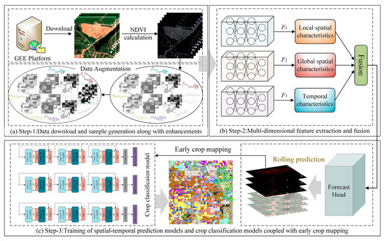
Figure 1.
Illustration of the general framework of the STPM, consisting of three main modules: (a) preparation and generation of time-series remote sensing data and sample augmentation, (b) extraction and fusion of multi-modal features from the samples, and (c) training of crop classification and spatial–temporal prediction models in combination with early crop mapping.
2.2. Local–Global–Temporal Multi-Modal Feature Exploration and Fusion
In order to effectively extract robust spatial–temporal evolving features of crops from remote sensing data, we have designed an integrated multi-modal feature extraction net-work architecture. Figure 2 shows an intuitive representation of the proposed network architecture. This model takes randomly cropped spatial–temporal patches as input samples, followed by an in-depth analysis of the recursive characteristics of remote sensing time-series data for future data generation. From various perspectives, such local–global–temporal multi-modal features are able to explore the spatial–temporal evolution patterns of crops for better simulation. Specifically, when the input sample (where H and W represent the height and width of the input patch, and T represents the length of the temporal dimension) enters the feature extraction network, it is extracted by multiple different feature extraction backbone networks for corresponding modal features. For local-scale features, the model uses a shallow depth separable convolution network (DSC) as the feature extractor. Compared with commonly used backbones [34,35], the DSC network can reduce the required training parameters while ensuring efficient feature extraction. For the input sample, this feature extraction stage includes two processes, namely convolution over time (DT) and convolution over pixels (PC). In the DT stage, n (n = T) 3 × 3 two-dimensional convolution kernels are used to perform sliding convolution on different temporal nodes to obtain the feature that is consistent with the initial dimension of the sample. The calculation process can be represented as . Then, based on feature , feature aggregation calculations are performed for each pixel using C convolution kernels of size 1 × 1 × T, resulting in the local-scale feature F1. The calculation involved can be represented as , where represent two different convolution operations. This network branch is used to extract local texture features from the sample. We set the depth of the final output feature to be C.
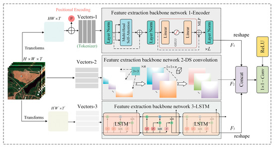
Figure 2.
Details of the multi-modal feature extraction process in the spatial–temporal prediction modular. Specifically, the input samples are extracted by three feature extraction backbone networks simultaneously for the corresponding types of features. These extracted features are then fused together by a deep feature fusion module.
For the extraction of global-scale features for the spatial dimension, we used the Transformer model as the feature extraction backbone network. The input sample x is first reshaped and flattened into a two-dimensional vector , and then a two-dimensional convolution layer is used to project the feature dimension of the vector to D, resulting in a feature vector . To maintain the order of the sequence within the sample and reduce the computational cost of the model, the backbone network preserves the original 1-D position embedding module. Specifically, a fixed position vector p is added to the feature vector to obtain a feature vector of the same dimension. Finally, the feature vector is fed into the stacked encoders, and the corresponding weight information is obtained through the attention mechanism. The internal structure of the encoder is shown in Figure 2. From the figure, it can be seen that each encoder layer consists of a Multi-Head Self-Attention (MHSA) module, an MLP module, and three Layer Norm (LN) layers. Meanwhile, the MLP module is connected by two fully connected layers and a GeLU activation function. Therefore, the entire process of obtaining the final global spatial feature representation F2 from the vector through the encoder can be expressed in the formula as follows:
In this equation, l denotes the number of layers in the encoder, and . Q, K, and V represent the projections of input feature vectors in different feature vector spaces, which are used to compute similarity and output vectors. Wi represents the corresponding projection parameter, while Hi denotes the distinct heads in the attention mechanism.
Finally, to effectively extract temporal features from the samples, a set of LSTM layers is integrated into the framework for temporal feature extraction. Specifically, the input sample x is continuously passed through interconnected LSTM cells, allowing the model to iteratively learn the temporal patterns within the data. Within each cell unit, the flow and propagation of information are controlled using forget gates (), input gates (), and output gates (), while the cell state () is used to capture and store temporal features. In summary, the process of obtaining temporal features F3 within the samples using the LSTM feature extraction backbone can be represented by the following equation:
where denotes the current moment of the hidden state inside the cell.
Once the local–global–temporal features are extracted, we concatenate all the resulting feature vectors to form a fused feature vector. In order to enhance the coupling relationship between the fused features, we design a simple feature aggregation module based on the fused feature. In particular, we use one-dimensional convolution and ReLU activation function in sequence to aggregate information of the concatenated feature, resulting in the final fused feature U. The specific process is shown in Equation (7).
In contrast to simple time-series prediction, in order to enable the model to learn robust spatial–temporal features that characterize the complex remote sensing scenes, we performed rolling training strategy along the temporal axis with representative samples. The training process is shown in Figure 3.
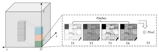
Figure 3.
Illustration of spatial–temporal rolling training.
Assuming that the input sample can be represented as , where denotes the two-dimensional spatial data at the i-th time node, we set a fixed temporal length K, which represents the two-dimensional spatial data containing K temporal nodes included in each sliding input, denoted as . At the same time, we take the center pixel value of the data corresponding to the K+1 node as the target label for the model. Once the current training step is finished, the model will continue to roll down within the batch of samples and obtain the second training sample, denoted as , while taking the center pixel value of the K + 2 node as the new target label. The advantage of training the model in this way is that it not only enables infinite rolling prediction of future data, but also allows the spatial–temporal prediction model to be unrestricted by the initial length of input time-series data.
Finally, the model feeds the aggregated feature U into a fully connected layer to predict the corresponding future pixel values. During this process, the algorithm utilizes the root mean square error (RMSE) as the loss function to continuously optimize and guide training process. The calculation method of the RMSE can be expressed as Equation (8).
where represent the predicted and true values, respectively, and N denotes the number of samples.
2.3. Spatial–Temporal Prediction for Early Crop Mapping
The spatial–temporal prediction module mentioned in the previous section was conducted to obtain future remote sensing data at the early growth stage of crops. Compared with existing early crop mapping methods [17,18,19], the STPM framework aims to forecast crop growth patterns step-by-step with current remote sensing data and perform early crop type mapping at the same time. The corresponding processing flow is shown in Figure 4.
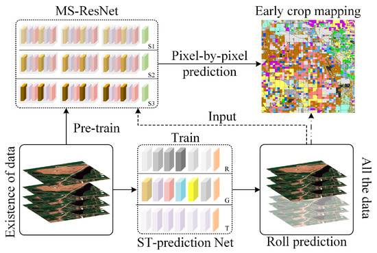
Figure 4.
Illustration of the STPM framework for collaborative processing, where MS-ResNet represents the crop identification module, and ST-prediction Net denotes the spatial–temporal prediction module.
Due to the inherent differences in training methods between the crop type identification module and spatial–temporal prediction module, it is necessary to pre-train a universal and transferable crop identification model. Considering the inter-annual growth variability of crops, in order to obtain a robust crop classification model, we trained a robust crop identification model based on a large number of time-series crop samples over the past years. Compared to existing time-series classification models, the Multi-Scale 1D ResNet (MS-ResNet) [36] classification network was chosen as the basic model for crop identification module due to its smaller network parameters, superior crop recognition ability, and model transferability. The MS-ResNet refers to the process of extracting features at different time scales from the input vector using multiple one-dimensional convolution kernels of different sizes, and then fusing all the scale features for subsequent crop classification tasks. Assuming that the convolution kernel sizes of the multi-scale convolution layer are and the corresponding convolution step sizes are , the process of extracting multi-scale features can be represented as follows,
Throughout the model training, the cross-entropy was adopted as the loss function, as formulated in Equation (11).
Among them, ReLU represents the activation function, BN stands for Batch Normalization layer, and denote the true crop label and the predicted result of the model, respectively.
Finally, assuming that the time-series remote sensing data available to us in the current year are , and the future time-series data to be predicted are . The final mapping result obtained through the proposed early crop mapping framework can be represented by
3. Materials
3.1. Study Area and Ground Reference Data Introduction
The test area selected for this experiment is located in California, United States, as shown in Figure 5. California, located on the west coast of the United States, has a population of approximately 39.5 million and a geographic area of approximately 414,000 square kilometers, making it the third-largest state in the USA. Due to its proximity to the Sierra Nevada Mountains and its location along the Pacific Ocean, the Central Valley has abundant water and thermal resources, providing excellent growing conditions for economically important crops such as fruits and vegetables. This has made California one of the most important agricultural states in the USA. According to official US statistics, the major crops planted in California in 2022 include almonds, walnuts, grapes, tomatoes, and winter wheat [37]. Within this state, we selected an area of interest, a 40 × 40 km crop plantation area in Fresno County. This plot is mainly used for growing economically important crops such as cotton, winter wheat, alfalfa, tomatoes, and grapes, and its corresponding crop calendar is described in Appendix A.
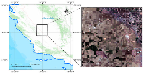
Figure 5.
Illustration of the study area, where the left map shows the geographical location of the study area, and the right map shows the actual surface distribution.
The Cropland Data Layer (CDL) [38] is a nationwide dataset created by the United States Department of Agriculture (USDA) using remote sensing, drone imagery, and ground sampling data. The CDL dataset provides information on crop planting and types across most of the United States, with higher spatial resolution. This dataset is not only valuable for agricultural decision-makers and policymakers but also has broad applications in fields such as land use, environmental protection, and natural disaster monitoring. Therefore, we used the CDL data of the study area as the ground reference data for training our crop classification model. Simultaneously, we pre-sampled the CDL data to a spatial resolution of 10 m using the nearest neighbor method to better match the remote sensing imagery.
3.2. Satellite Data Download and Pre-Processing
To test the effectiveness of the STPM, we utilized the widely used NDVI time-series data as the background data for spatial–temporal prediction and crop identification. To this end, we obtained multiple years of NDVI time-series remote sensing data with a time span from 1 January 2019 to 31 December 2022, using the S2 Level-2A data obtained from the Google Earth Engine (GEE) [39] cloud platform under limited conditions of time, cloud cover, and cloud masks (with QA60 band markers). Optical remote sensing data is often affected by cloud cover, which can lead to differences in the amount of effective data available and the time intervals between adjacent data for the same area in different years, thereby interfering with the evaluation of subsequent spatial–temporal prediction and crop identification models. To address this issue, we used the 10-day median synthesis method to synthesize multiple scenes, where all available data for a fixed time window of 10 days are arranged from smallest to largest. Then, the median of all data for these 10 days is taken as the composite value, and the results are stored, thus ensuring that the effective data length for each year in the study area remains at 37 scenes. Finally, we applied S-G filtering [40] to the synthesized data with an initial window size of seven iterations to fill in missing values in the time-series data, reducing the impact of noise or outliers during the model training process.
Figure 6 shows the rules set for the synthesis of data. Assuming that the latest S2-NDVI data on the GEE platform is the 20th synthesized scene in 2022, and three years of CDL data from 2019 to 2021 can be obtained as crop labels, we trained and tested the STPM model based on these data after necessary pre-processing.
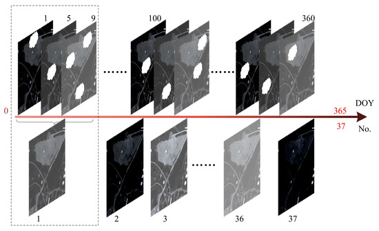
Figure 6.
Rules for data synthesis. The sequences from left to right represent time-series data within a year, where the dashed boxes indicate the synthesis process of ten days.
3.3. Sample Acquisition and Splitting
For the crop classification module, we first statistically analyze the proportions of different crop types based on historical label data and then reclassify them, as shown in Table 1. Although crop rotation occurs in the agricultural areas of the USA, the main crop types in the research area remain relatively stable across different years. Therefore, we reclassified the main crop types in the research area into 12 categories. On this basis, we take a random sampling within each year to extract the NDVI time-series data and labels corresponding to each sample point. Specifically, we used the CDL data as a reference and took a random scattering of points on top of it to obtain the samples, where the number of samples selected was 0.5% of the total number of pixels. Finally, all crop samples from different years were mixed and randomly divided into mutually independent training, testing, and validation sets at a ratio of 5:3:2.

Table 1.
Real crop type distribution in the study area and selection of main crop types (“Others” represents the total proportion of all crop types that account for a relatively small percentage compared to the entire study area, and “Impervious” represents all impervious surfaces).
Unlike the training mode of the classification model, when generating spatial–temporal prediction samples, we first overlay the NDVI time-series data from 2019 to 2022 (with 20 scenes) and then randomly cut out 17 × 17 tiles on the original data at a certain ratio. In order to balance the sample size and the generalization ability of the model, we performed data augmentation on the obtained tiles using commonly used methods such as rotation, translation, and adding noise. Finally, we divided the samples into mutually independent training, testing, and validation sets at a ratio of 5:3:2, consistent with the splitting of classification samples. Table 2 and Table 3 show the respective distributions of the two types of samples.
Table 2.
The number of samples for each crop type listed in the table refers to only one of the three years 2019–2021, so the number of samples used to train the crop classification model (including the training, validation, and test sets) is equal to the number in the table multiplied by 3.
Table 3.
Division of spatial–temporal prediction sample quantity distribution.
3.4. Experimental Design and Model Parameter Configuration
To better capture the spatial–temporal evolution patterns of the crops, we designed multiple feature extraction channels to obtain multi-modal feature information. Specifically, in each stage of training, the model slides to extract input samples within multiple spatial–temporal tiles, with a size of 4 × 17 × 17, and takes the center pixel of the corresponding next time node as the output label. For local feature extraction, the network uses four convolution kernels of sizes 3 × 3 and 1 × 1 to extract local feature vectors, which are then stretched into a size of 4 × 289. In addition, for the Transformer component, the model sets up 6 layers of encoders, with the heads of the multi-head attention set to 17 and the input dimension of the feed-forward network set to 289. Finally, a global feature vector of size 5 × 289 is outputted. For the temporal feature extraction branch, the input dimension is set to 289, the hidden nodes are set to 64, the network layers are set to 3, and the output feature size is set to 4 × 289. After all the feature extraction is completed, the multi-modal features are concatenated to form a fusion feature vector of size 13 × 289, and then an information aggregation is performed using a one-dimensional convolution kernel of size 1 × 13 to obtain a final feature vector of size 1 × 289.
Regarding crop classification, the model takes an input crop time-series of size 1 × 37 and uses 64 1 × 3, 1 × 5, and 1 × 7 convolution kernels to extract features of different scales. These features are then passed through multiple BN layers, ReLU layers, and convolutional layers. Next, multiple mean pooling layers are used to reduce the dimensionality of the extracted multiscale features to a size of 1 × 18. Finally, the features of different scales are concatenated and passed through fully connected layers and activation layers to output crop category information.
All of the modules described above were trained using the PyTorch framework [41]. The Adam optimizer was used for training all models, with default settings of beta_1 = 0.9, beta_2 = 0.999, and epsilon = 1 × 10⁻⁸. For the crop classification model, we set the initial learning rate to 0.0001, batch size to 256, and trained for 100 epochs. For the spatial–temporal prediction model, we set the initial learning rate to 0.001, batch size to 512, and trained for 256 epochs. To prevent overfitting during the training process, we employed an early stopping mechanism to obtain the optimal set of model parameters. Model training was conducted on a server with the CentOS 7.6 operating system, an Intel(R) Xeon(R) Gold 5118 CPU, and two NVIDIA Tesla 100 16G graphics cards. The training process used Python version 3.7.
3.5. Model Evaluation Indicators
To better evaluate the potential of the proposed STPM methods in the paper, we used different evaluation metrics to assess the spatial–temporal prediction module and crop classification module, respectively. For the proposed spatial–temporal prediction module, we used RMSE as the evaluation metric to judge the model’s training performance during the training phase. When the model made predictions, we also added R2 as an evaluation metric. As for the crop identification module, we used five commonly used accuracy evaluation metrics, including accuracy, precision, recall, F1-score, and Kappa coefficient, to assess the training accuracy and prediction capabilities. In detail, we used accuracy to evaluate the pre-trained crop classification model from an overall perspective. Recall and precision were selected to assess the model’s ability to distinguish between positive and negative samples, and finally, we used F1-score and Kappa coefficient as two comprehensive metrics to evaluate the model’s robustness.
4. Results
4.1. Evaluation of Spatial–Temporal Prediction Results
In this section, we employed our proposed spatial–temporal prediction model to forecast the spatial–temporal distribution of S2-NDVI in the selected study area from day 210 to 365 in 2022. To evaluate the performance of the model in predicting remote sensing time-series data, we conducted qualitative and quantitative evaluations. At the qualitative level, we visualized the spatial–temporal prediction results of the first nine prediction scenes and assessed the spatial pattern of the model from various aspects, including the degree of surface texture preservation. Meanwhile, we quantified the NDVI prediction results at each temporal node and the overall prediction results using multiple evaluation methods, such as density scatter plots, R2, and RMSE. Finally, we conducted a comparative analysis of the prediction errors of different crop types from different aspects.
Figure 7 presents the NDVI prediction results of the selected study area for days 210–300 in 2022. All spatial predictions of the model are very similar to the real surface distribution in visual inspection. The boundaries of cultivated land and field contours can be accurately distinguished on the map, proving the potential of our proposed spatial–temporal prediction module for large-scale prediction even in complex regions. For the fragmented and heterogeneous regions, as shown in the red box of Figure 7, the proposed method is able to capture the evolution pattern from the spatial–temporal domain, keeping spatial details in all nine prediction maps. In addition, we will discuss the impact of heterogeneity on the prediction results in depth in the following section.
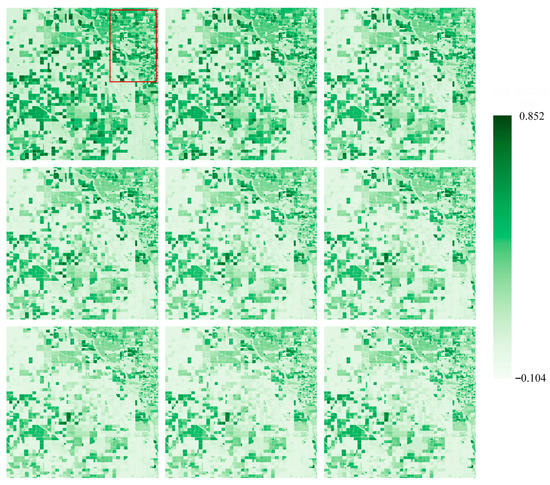
Figure 7.
The spatial-temporal prediction results of the NDVI data, based on our proposed model, are presented using a pseudocolor visualization. From left-up corner to right-down corner, they represent the 21st to 30th scenes of the synthesized data in 2022, corresponding to the real-time span of 210–300 days in 2022.
In Figure 8 and Figure 9, we quantitatively analyze and evaluate the prediction results from two aspects: density scatter plot and error histogram. These measures clearly demonstrate the similarity between the predicted NDVI time-series data and the real time-series data for the first nine predicted scenes. From the distribution of the density scatter plots and the statistics of R2 and RMSE, we can see that the scatter plot distributions corresponding to the predicted data from the first scene to the ninth scene are gradually diverging towards both ends, with a clear downward trend in R2 and a significant increase in RMSE. These results indicate that as time goes on, the prediction accuracy of the model gradually decreases. This is an understandable phenomenon for any rolling prediction model because every prediction process of the model will introduce certain errors. As the prediction length increases, the accumulated error also increases, leading to worse prediction results. Still, our proposed model outperforms most existing spatial–temporal prediction networks in terms of prediction accuracy and maximum effective prediction time, which will be discussed in Section 4.2. Meanwhile, we can also observe from the change of the scatter plots that although the distribution range of the scatter plot increases with the increase of the prediction length, most of the red hotspots shown in the figures are distributed on the diagonal, and their relative positions in the figure are continuously decreasing along the line. Considering that the starting time of our prediction model was around the end of June to early July 2022, which is close to the peak growth and harvest periods of most crops in the study area, most NDVI values corresponding to the initial time-series data for prediction are relatively high and gradually decrease as time goes.
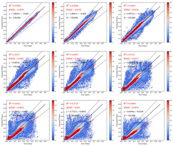
Figure 8.
Scatter plot results of partial NDVI prediction and actual data. A total of 150,000 representative pixels were randomly selected from the predicted image and the corresponding real image to calculate their R2, average RMSE, and fitting function relationship. The time range corresponds to that in Figure 7.
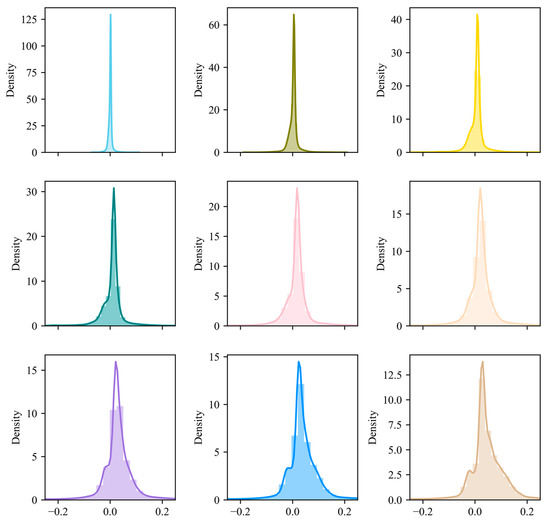
Figure 9.
Histogram statistics of the error of the top nine scenes of NDVI prediction.
The histogram of prediction errors (the difference between the true value and the predicted value) for each predicted scene shows that the errors of the first nine scenes are concentrated within the range of (−0.2, 0.2) and almost follow a normal distribution. This undoubtedly indicates that the proposed model has a good predictive ability. When we observe the prediction errors along the time axis, we can see that the corresponding kernel density curve gradually widens and moves towards the positive direction with the in-crease in time, indicating that the corresponding standard deviation is continuously increasing, and the predicted values are gradually decreasing compared to the true values. This provides us with ideas and information sources for future improvement of the model.
In response to the previous question, to explore the impact of surface heterogeneity on the prediction results, we used a trained spatial–temporal prediction model to perform rolling prediction of the remaining 17 scenes of NDVI data in the study area in 2022 and overlaid them in chronological order. Based on this model, we obtained the spatialized results shown in Figure 10 by calculating the R2 and RMSE between the predicted temporal data and the actual results on a pixel-by-pixel basis.
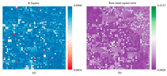
Figure 10.
(a) and (b) respectively illustrate the R2 and RMSE calculation results between the predicted NDVI time-series based on the proposed model and the actual time-series data.
Combining Figure 10a,b, it can be found that there are a few outliers in the flat and homogeneous cultivated land blocks, and these outliers exhibit a clear block distribution phenomenon. Considering that different crop types are planted in this area, there are significant differences in the growth and development patterns of different crop types (The anomalous areas are mainly found in plots planted with the three crop types, alfalfa, others, and fallow). This error distribution phenomenon may be related to the crop types planted in the parcel, which is also confirmed in our discussion of the impact of different crop types on the prediction results later. Compared with the vast majority of homogeneous and regular parcels, the prediction errors in the surface fragmented area corresponding to the red box are generally at a relatively high level, which indicates that the higher the degree of surface heterogeneity, the more errors are introduced during prediction.
In the previous discussion, we mainly analyzed and evaluated the accuracy of the prediction model at the spatial scale. However, the ultimate goal is to achieve early crop mapping based on remote sensing data through spatial–temporal prediction. Assuming that the crop classification model established can accurately identify all crop types, the prediction ability of the model will directly affect the accuracy of crop mapping. With this assumption, we refer to the CDL data and randomly select 300 sample points for each crop type based on the complete temporal prediction data obtained prior. We then calculate the average error between the predicted data and the actual data and display it in a violin plot.
Based on the quantitative indicators in Figure 11, it can be seen that the median of the average error of most crop types in the study area is distributed around 0. However, the distribution of prediction errors for different crop types in the figure varies significantly, which confirms our previous hypothesis that the prediction accuracy of spatial–temporal prediction models is related to crop types. Specifically, the average prediction errors for fallow, garlic, and onions are clearly represented by a “short and thick” violin plot in the figure, indicating that the spatial–temporal prediction model performs quite well in predicting the spatial–temporal changes of these three crop types. After comparing and analyzing the NDVI values of the three crop types from the 21st to 37th scenes, we found that these three crop types have a common characteristic: they are generally near their lower value during the year. This indicates that the model is sensitive to low values, which is consistent with the fact that the predicted values are generally lower than the true values, as reflected in the error histogram. For the five crop types of almonds, pistachios, winter wheat, tomatoes, and grapes, their corresponding average error violin plots exhibit a relative regularity. This is because their NDVI curves during this period show a process of decreasing from high values to low values, and the low sensitivity of the prediction model to high values leads to an expansion of the error. Finally, for the four types of cotton, alfalfa, impervious, and others, we can see clearly from Figure 11 that their corresponding violin plots are wide and long, indicating that there is a large difference in the average prediction errors among these types and a wide distribution range. Upon closer examination, the poor prediction performance of the model can be attributed to the fact that impervious, others, and alfalfa are not single crop types, making it difficult for the model to learn a stable spatial–temporal evolution pattern within them. Compared with the NDVI regularity changes of other crop types, the high value duration of cotton occupies the vast majority of the predicted time. Combining the previous analysis and error accumulation effects, the relatively scattered average prediction error of cotton can also be explained.
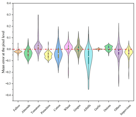
Figure 11.
The violin plot represents the distribution of prediction errors for different crop types, where the white dot indicates the median of the error distribution, the width of the violin represents the frequency distribution of the prediction errors, and the thin black lines inside the violins indicate the range between the minimum and maximum values.
4.2. Comparative Experiment Based on Spatial–Temporal Prediction Models
To evaluate the superiority of our model in spatial–temporal prediction of fine-scale remote sensing data, we compared our proposed model with other spatial–temporal prediction models in this section. Since our model is trained based on the spatial–temporal sequence-to-pixel approach, it is difficult to find competitors with similar techniques. Therefore, based on existing research, we selected four competitive models for comparison, namely Memory In Memory (MIM) [42], ConvLSTM [43], PredRNN [44], and CubicRNN [45]. Simultaneously, to ensure fairness in the comparison, we used the same set of samples for all models and kept the training method unchanged. Table 4 summarizes the relevant information for all the models used in the experiment.
Table 4.
Brief summary of the comparison of model structures, including MIM, ConvLSTM, PredRNN, and CubicRNN.
By observing Table 4, it can be seen that different spatial–temporal prediction models use different building blocks, while almost all of them involve convolution and LSTM computing units internally. Once all models were well-trained, we selected the best training parameters for each model to conduct rolling prediction on S2-NDVI data and summarized the prediction accuracy of all models at each temporal point in Table 5. Regarding Table 5, we first conducted a vertical self-comparison of the four comparison models and found that, except for the ConvLSTM model, the effective prediction length of the remaining three comparison models is only up to the third scene, and the R2 of predicting the first scene data is not higher than 0.9. This indicates that these three models cannot effectively learn the spatial–temporal evolving rules of large-scale remote sensing data, and their predictive capabilities for unknown remote sensing data are generally weak. The ConvLSTM model has a relatively excellent prediction ability, which may be due to its wide range of applicability and strong spatial–temporal modeling ability. Then, we continued to conduct horizontal comparisons of the prediction results of these four models with the model proposed in this article. It can be clearly seen that our proposed model has an advantage in both the effective length of prediction and the accuracy at each time point. At the same time, the decline rate of the prediction accuracy of all comparison models is significantly higher than that of our proposed model, which indirectly indicates that these models are more sensitive to error accumulation on spatial–temporal scales and have weaker robustness.
Table 5.
Comparison of the accuracy of spatial–temporal prediction models. We set the R2 value of 0.30 as the threshold for determining the validity of the prediction results. Any predictions below this threshold are considered invalid and denoted by a “-” in the table. The same threshold is used for Table 6.
4.3. Early Crop Mapping Accuracy Assessment
In the process of large-scale crop mapping, the training of the crop identification model is crucial as it directly affects the accuracy of the down-stream crop mapping task. Therefore, we first evaluated the training effectiveness of the crop classification model used based on the hyperparameters determined in the previous chapters. Among them, Figure 12 illustrates five evaluation metrics for crop classification accuracy during the training process and the trend of the loss function on the validation set. We can clearly see that the model’s loss function has become stable by around the 40th epoch, and the overall validation accuracy is maintained at around 80%. To improve the generalization ability of the model, we trained a classification model on a collection of crop samples from multiple years, as mentioned in the previous section, in order to enhance its robustness. Combining prior conditions such as label quality and sample type distribution, the final validation accuracy of the classification model is acceptable.
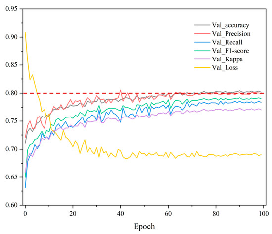
Figure 12.
Changes in various accuracy evaluation metrics and loss function on the validation set as the number of epochs increases during crop classification model training.
At the same time, Figure 13 shows the confusion matrix on the validation set in the last training stage. From the figure, we can see that, except for the relatively poor training accuracy of winter wheat and impervious, the training effectiveness of other crop types is still satisfactory.
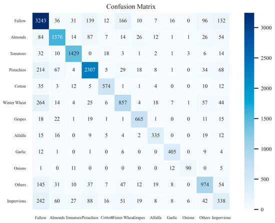
Figure 13.
Confusion matrix results on the validation set during crop classification model training.
Finally, based on the time-series prediction data obtained in the upper section, we combined the known NDVI time-series data of crop early growth with the predicted results and input them into the crop identification model for prediction, obtaining the crop early mapping results shown in Figure 14. From the figure, we can see that the predicted results are filled with a small amount of noise, and the prediction accuracy of the impervious type is very low, which is consistent with the information displayed in the confusion matrix. This may be due to the weak correlation between the predicted data and the real data. As a result, the NDVI values corresponding to the impervious surfaces gradually decreased over the year from being relatively stable to less stable, and when the cumulative errors between the data exceeded the tolerance range of the crop identification model, recognition errors occured. However, for major crop types such as almonds, tomatoes, and cotton, we can visually observe that the model’s recognition accuracy has reached an acceptable level when the initial length is only 20 in 2022. By observing the annual growth curves of different crop types, it can be inferred that the pre-trained crop classification model mainly focuses on the growth peak range [46]. Therefore, it is not difficult to conclude that the longer the time span of known remote sensing data, the higher the recognition accuracy, which is discussed in detail in Section 5.2.
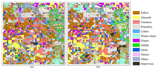
Figure 14.
(a) Visualization of the early crop mapping results in 2022 by combining existing NDVI data with spatial–temporal prediction results. (b) Distribution of actual crop types in 2022.
5. Discussion
5.1. Contribution Evaluation of Multi-Modal Features to the Spatial–Temporal Prediction Module
To better evaluate the contribution of multi-modal features to S2-NDVI spatial–temporal prediction, we trained and predicted the model based on local, global spatial features, and temporal features, respectively, while ensuring that the input data and hyperparameters were the same. Figure 15 shows the corresponding loss function changes of these four models during the validation set training. Several rules can be observed from the figure. Firstly, our proposed model showed the fastest decrease in the loss function during training, followed by the time-based model, while the model that used ViT solely as the feature extraction backbone performed the worst. The second point is that the models based on multi-modal features and temporal features showed a decreasing trend in the loss function during training, while the models based on local and global features exhibited multiple fluctuations in the loss function, indicating that these two models had poor fitting performance and could not effectively learn the temporal and spatial patterns of the data. After all models were trained, we performed rolling predictions along the temporal axis based on their respective best training parameters and evaluated the prediction accuracy. The results are summarized in Table 6.
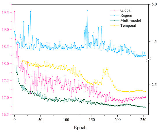
Figure 15.
Changes in the loss function of the spatial–temporal prediction model based on different features during training on the validation set. As the numerical differences corresponding to the stable state of loss reduction during the training process of different models are too large to be displayed effectively, a double y-axis line graph is used to show the differences between the models. Each model is represented by a different color, and except for the pink line, which is referenced to the left axis, the other three lines are referenced to the right axis.
From Table 6, it is clear that the model based on multi-modal features for spatial–temporal prediction has significant advantages in both prediction accuracy and effective prediction length, which directly proves the validity of our proposed viewpoint. Secondly, for single-feature prediction, the model based on temporal features performs best for S2-NDVI data, while the model based on global spatial features performs the worst. Although there are many improved versions of ViT models that have achieved excellent results in video prediction and other areas [47,48], our experiments demonstrate that the Transformer itself is not particularly suitable for spatial–temporal prediction of fine-scale remote sensing data. Finally, we can conclude that for our proposed spatial–temporal prediction model, temporal features play a dominant role in the entire learning process, while local and global spatial features serve as auxiliary learning factors.
Table 6.
Comparison of accuracy for spatial–temporal prediction models based on multi-modal and single features.
Table 6.
Comparison of accuracy for spatial–temporal prediction models based on multi-modal and single features.
| Feature | Local | Global | Temporal | Local–Global–Temporal | |
|---|---|---|---|---|---|
| R2-RMSE | |||||
| 21 | 0.9855–0.0224 | 0.7225–0.0981 | 0.9979–0.0086 | 0.9982–0.0078 | |
| 22 | 0.9427–0.0433 | 0.3187–0.1492 | 0.9870–0.0206 | 0.9886–0.0192 | |
| 23 | 0.8413–0.0696 | - | 0.9595–0.0351 | 0.9631–0.0036 | |
| 24 | 0.5955–0.1065 | - | 0.9102–0.0500 | 0.9170–0.0482 | |
| 25 | - | - | 0.8431–0.0637 | 0.8447–0.0633 | |
| 26 | - | - | 0.7675–0.0746 | 0.7630–0.0757 | |
| 27 | - | - | 0.6628–0.0848 | 0.6611–0.0853 | |
| 28 | - | - | 0.5664–0.0915 | 0.5724–0.0910 | |
| 29 | - | - | 0.4765–0.0976 | 0.4949–0.0954 | |
| 30 | - | - | 0.3883–0.1044 | 0.4168–0.1018 | |
| 31 | - | - | - | 0.3653–0.1031 | |
| 32 | - | - | - | 0.3221–0.1022 | |
| 33 | - | - | - | 0.3137–0.0952 | |
| 34 | - | - | - | 0.3546–0.0794 | |
| 35 | - | - | - | 0.3566–0.0632 | |
| 36 | - | - | - | - | |
| 37 | - | - | - | - | |
5.2. The Impact of Initial Sequence Length on Early Crop Mapping Accuracy
The initial length of the input data directly affects the training effectiveness of spatial–temporal prediction models. In the preceding experimental section, all experiments were conducted with an initial length of 20 in the year 2022. To investigate the impact of the initial sequence length on crop mapping accuracy, we deliberately increased or decreased the original input length by five-time steps while keeping other hyperparameters the same and trained the model accordingly. Subsequently, the trained model was used to make rolling predictions on the input of the next step. Finally, the three stacked NDVI time-series data were fed into the same trained crop identification model for large-scale crop spatial mapping, and the corresponding mapping accuracy was statistically analyzed. The mapping and statistical results are shown in Figure 16 and Table 7, respectively.
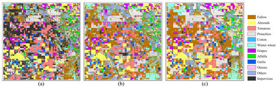
Figure 16.
Early crop mapping results corresponding to different initial data lengths, where (a–c) represent the available data lengths in 2022 as 15, 20, and 25, respectively.
Table 7.
Comparison of early crop mapping accuracy for different initial training lengths (where data from 2019–2021 were used for training, the only difference being the length of available data in 2022).
Regarding the spatial crop mapping results, we can clearly see significant changes in the pattern. Firstly, the salt-and-pepper noises in the crop mapping results gradually decreased. Secondly, for some crop parcels, the initial misclassification or omission gradually shifted to correct classification as the initial length increased. This change was most evident for others and impervious types, while some crop types, such as almonds and pistachios, showed little difference. At the same time, from the quantitative indicators in Table 7, we can see that the identification accuracy of almost all crop types improved with the initial data extension. Even the identification accuracy of the other types increased from 0.44 to 0.75. Surprisingly, when the available data in 2022 reached 25-time steps (around mid-June), the early crop mapping framework we proposed almost achieved the same accuracy as that of using data for the entire year. This result confirms the effectiveness of our work. Clearly, these changes align with our initial hypothesis that the longer the initial data length, the better the spatial–temporal prediction model’s prediction effect and the lower the accumulated error.
5.3. Advantages and Limitations
Against the backdrop of a general lag in mapping research on most existing crops, researchers have begun to focus on early crop mapping. Although a small amount of work has been devoted to early crop mapping based on sample selection and feature selection, these methods are obviously not scalable. Instead, the STPM framework starts from the spatial–temporal prediction of remote sensing data, combined with historical time-series data and crop identification models, fundamentally alleviating the problem of lack of data in the early stages of crop growth. We also analyzed the applicable scope of the spatial–temporal prediction model and the reliable time for early crop mapping from both qualitative and quantitative perspectives, comprehensively exploring the outstanding advantages of the STPM early crop mapping framework in crop mapping production.
However, there are several shortcomings in this work. Firstly, the STPM framework requires a significant amount of computational time and running costs for training, as well as a large sample size. This is because the training of time-series prediction models requires continuous learning of internal changes in data across multiple feature dimensions, and fine-scale remote sensing data contains much more information than other types of data, such as video data. Secondly, the model itself lacks an error correction mechanism. From the above result analysis, we found that unlimited rolling prediction without restrictions leads to a rapid accumulation of prediction errors and a sharp decrease in prediction accuracy. Finally, our proposed STPM model is based on many years of historical remote sensing data and ignores various extreme factors to learn the near-stable spatial–temporal pattern of crop changes, so it is difficult to predict abnormal changes in crop growth caused by sudden natural disasters. In future work, we will focus on lightweight models and error correction mechanisms to achieve timely detection of crop information.
6. Conclusions
This study proposes a novel deep learning framework for fine-scale remote sensing data prediction and early crop mapping. The results of the experiments demonstrate that our proposed spatial–temporal prediction module can achieve high prediction accuracy in terms of future data generation, even in heterogeneous regions. Furthermore, the analysis of the prediction results shows that the prediction accuracy in the crop planting area is affected by crop types and the degree of surface heterogeneity. When compared to other competing spatial–temporal forecasting models, our model is able to outperform all of them in terms of effective forecast length of over 100 days, as well as forecast accuracy per view. Regarding large-scale early crop mapping, we analyzed the impact of different initial sequence lengths on crop mapping accuracy and examined the transfer effect of pre-trained crop recognition models over time from multiple perspectives.
In summary, this study provides a new deep learning framework for early crop mapping to alleviate the problem of information lag due to the lack of early crop growth data. However, there are still a few issues with this method that need further improvement, for example, the accumulation of errors when the spatial–temporal prediction model is rolling for a long time, etc.
Author Contributions
K.L. constructed the experimental framework and gathered datasets of the study area; W.Z. conceived the idea of the STPM; J.C. and L.Z. helped with the experiments and analysis of results; Q.W. and D.H. offered help with paper revision and language proofreading. All authors have read and agreed to the published version of the manuscript.
Funding
This work is supported by the National Natural Science Foundation of China (62201063), the National Natural Science Foundation of China Major Program under Grant (42192580, 42192584), and Alibaba Innovative Research (AIR) project.
Data Availability Statement
The data that support the findings of this study are available from the corresponding authors upon reasonable request.
Conflicts of Interest
The authors declare no conflict of interest.
Appendix A. Introduction to the Crop Calendar
Figure A1 illustrates the harvest time frames of major crop types within the study area across California. Overall, most crops exhibit maturity periods primarily ranging from June onwards, with varying durations of two to five months. Additionally, due to the shorter growth cycles of crops such as alfalfa, onions, and tomatoes, which can be cultivated multiple times within a year, they demonstrate longer maturity periods.

Figure A1.
Diagram showing the harvesting calendar for each of the major crops in the study area.
Simultaneously, the following outlines the distribution of planting periods for the aforementioned crop types:
Almonds: Planting of almonds typically commences between February and March.
Tomatoes: The planting time for tomatoes varies by variety and region. Early-season tomatoes are typically sown from late February to early April, while late-season tomatoes are planted between July and August.
Pistachios: Pistachios are typically planted between March and April.
Cotton: Cotton is typically planted between April and May.
Winter wheat: Winter wheat is usually sown between October and December.
Grapes: The planting time for grapes varies by variety and region, generally beginning in spring, specifically from late February to early April.
Alfalfa: Alfalfa is typically planted between March and May.
Garlic: Garlic is typically planted between October and November.
Onions: Onions are usually planted between February and March.
However, it should be noted that actual planting times may vary due to factors such as geographical location, climatic conditions, and cultivation goals. The aforementioned planting and harvest time periods serve as a general reference.
References
- Milner, G.R.; Boldsen, J.L. Population trends and the transition to agriculture: Global processes as seen from North America. Proc. Natl. Acad. Sci. USA 2023, 120, e2209478119. [Google Scholar] [CrossRef]
- Pinstrup-Andersen, P. Challenges to agricultural production in Asia in the 21st Century. In Water in Agriculture; ACIAR Proceedings No. 116; Australian Centre for International Agricultural Research: Canberra, Australia, 2004. [Google Scholar]
- Fontanelli, G.; Crema, A.; Azar, R.; Stroppiana, D.; Villa, P.; Boschetti, M. Agricultural crop mapping using optical and SAR multi-temporal seasonal data: A case study in Lombardy region, Italy. In Proceedings of the 2014 IEEE Geoscience and Remote Sensing Symposium, Quebec City, QC, Canada, 13–18 July 2014; pp. 1489–1492. [Google Scholar]
- Hao, P.-Y.; Tang, H.-J.; Chen, Z.-X.; Meng, Q.-Y.; Kang, Y.-P. Early-season crop type mapping using 30-m reference time series. J. Integr. Agric. 2020, 19, 1897–1911. [Google Scholar] [CrossRef]
- Osman, J.; Inglada, J.; Dejoux, J.-F. Assessment of a Markov logic model of crop rotations for early crop mapping. Comput. Electron. Agric. 2015, 113, 234–243. [Google Scholar] [CrossRef]
- Yaramasu, R.; Bandaru, V.; Pnvr, K. Pre-season crop type mapping using deep neural networks. Comput. Electron. Agric. 2020, 176, 105664. [Google Scholar] [CrossRef]
- Lin, C.; Zhong, L.; Song, X.-P.; Dong, J.; Lobell, D.B.; Jin, Z. Early-and in-season crop type mapping without current-year ground truth: Generating labels from historical information via a topology-based approach. Remote Sens. Environ. 2022, 274, 112994. [Google Scholar] [CrossRef]
- Blickensdörfer, L.; Schwieder, M.; Pflugmacher, D.; Nendel, C.; Erasmi, S.; Hostert, P. Mapping of crop types and crop sequences with combined time series of Sentinel-1, Sentinel-2 and Landsat 8 data for Germany. Remote Sens. Environ. 2022, 269, 112831. [Google Scholar] [CrossRef]
- Kumar, S.; Meena, R.S.; Sheoran, S.; Jangir, C.K.; Jhariya, M.K.; Banerjee, A.; Raj, A. Remote sensing for agriculture and resource management. In Natural Resources Conservation and Advances for Sustainability; Elsevier: Amsterdam, The Netherlands, 2022; pp. 91–135. [Google Scholar]
- Zhao, W.; Wang, M.; Pham, V. Unmanned Aerial Vehicle and Geospatial Analysis in Smart Irrigation and Crop Monitoring on IoT Platform. Mob. Inf. Syst. 2023, 4213645, 2023. [Google Scholar] [CrossRef]
- Li, H.; Tian, Y.; Zhang, C.; Zhang, S.; Atkinson, P.M. Temporal Sequence Object-based CNN (TS-OCNN) for crop classification from fine resolution remote sensing image time-series. Crop J. 2022, 10, 1507–1516. [Google Scholar] [CrossRef]
- Sun, C.; Bian, Y.; Zhou, T.; Pan, J. Using of multi-source and multi-temporal remote sensing data improves crop-type mapping in the subtropical agriculture region. Sensors 2019, 19, 2401. [Google Scholar] [CrossRef]
- Virnodkar, S.S.; Pachghare, V.K.; Patil, V.; Jha, S.K. Application of machine learning on remote sensing data for sugarcane crop classification: A Review. In ICT Analysis and Applications; Proceedings of ICT4SD 2019; Springer: Singapore, 2020; Volume 2, pp. 539–555. [Google Scholar]
- Wei, S.; Zhang, H.; Wang, C.; Wang, Y.; Xu, L. Multi-temporal SAR data large-scale crop mapping based on U-Net model. Remote Sens. 2019, 11, 68. [Google Scholar] [CrossRef]
- Hu, Q.; Sulla-Menashe, D.; Xu, B.; Yin, H.; Tang, H.; Yang, P.; Wu, W. A phenology-based spectral and temporal feature selection method for crop mapping from satellite time series. Int. J. Appl. Earth Obs. Geoinf. 2019, 80, 218–229. [Google Scholar] [CrossRef]
- Wang, J.; Xiao, X.; Liu, L.; Wu, X.; Qin, Y.; Steiner, J.L.; Dong, J. Mapping sugarcane plantation dynamics in Guangxi, China, by time series Sentinel-1, Sentinel-2 and Landsat images. Remote Sens. Environ. 2020, 247, 111951. [Google Scholar] [CrossRef]
- Park, N.-W.; Park, M.-G.; Kwak, G.-H.; Hong, S. Deep Learning-Based Virtual Optical Image Generation and Its Application to Early Crop Mapping. Appl. Sci. 2023, 13, 1766. [Google Scholar] [CrossRef]
- Yi, Z.; Jia, L.; Chen, Q.; Jiang, M.; Zhou, D.; Zeng, Y. Early-Season Crop Identification in the Shiyang River Basin Using a Deep Learning Algorithm and Time-Series Sentinel-2 Data. Remote Sens. 2022, 14, 5625. [Google Scholar] [CrossRef]
- Yan, Y.; Ryu, Y. Exploring Google Street View with deep learning for crop type mapping. ISPRS J. Photogramm. Remote Sens. 2021, 171, 278–296. [Google Scholar] [CrossRef]
- Gao, F.; Zhang, X. Mapping Crop Phenology in Near Real-Time Using Satellite Remote Sensing: Challenges and Opportunities. J. Remote Sens. 2021, 2021, 8379391. [Google Scholar] [CrossRef]
- Chen, C.; Liu, Y.; Chen, L.; Zhang, C. Bidirectional spatial-temporal adaptive transformer for Urban traffic flow forecasting. IEEE Trans. Neural Netw. Learn. Syst. 2022, 1–13, early access. [Google Scholar] [CrossRef]
- Yang, R.; Srivastava, P.; Mandt, S. Diffusion probabilistic modeling for video generation. arXiv 2022, arXiv:2203.09481. [Google Scholar]
- Zhang, Q.; Feng, G.; Wu, H. Surveillance video anomaly detection via non-local U-Net frame prediction. Multimed. Tools Appl. 2022, 81, 27073–27088. [Google Scholar] [CrossRef]
- Zhou, T.; Huang, B.; Li, R.; Liu, X.; Huang, Z. An attention-based deep learning model for citywide traffic flow forecasting. Int. J. Digit. Earth 2022, 15, 323–344. [Google Scholar] [CrossRef]
- Azari, M.; Billa, L.; Chan, A. Multi-temporal analysis of past and future land cover change in the highly urbanized state of Selangor, Malaysia. Ecol. Process. 2022, 11, 2. [Google Scholar] [CrossRef]
- Nakapan, S.; Hongthong, A. Applying surface reflectance to investigate the spatial and temporal distribution of PM2.5 in Northern Thailand. ScienceAsia 2022, 48, 75–81. [Google Scholar] [CrossRef]
- Wang, D.; Cao, W.; Zhang, F.; Li, Z.; Xu, S.; Wu, X. A review of deep learning in multiscale agricultural sensing. Remote Sens. 2022, 14, 559. [Google Scholar] [CrossRef]
- Alhichri, H.; Alswayed, A.S.; Bazi, Y.; Ammour, N.; Alajlan, N.A. Classification of remote sensing images using EfficientNet-B3 CNN model with attention. IEEE Access 2021, 9, 14078–14094. [Google Scholar] [CrossRef]
- Seydi, S.T.; Hasanlou, M.; Amani, M.; Huang, W. Oil spill detection based on multiscale multidimensional residual CNN for optical remote sensing imagery. IEEE J. Sel. Top. Appl. Earth Obs. Remote Sens. 2021, 14, 10941–10952. [Google Scholar] [CrossRef]
- Wang, W.; Chen, Y.; Ghamisi, P. Transferring CNN with Adaptive Learning for Remote Sensing Scene Classification. IEEE Trans. Geosci. Remote Sens. 2022, 60, 5533918. [Google Scholar] [CrossRef]
- Ho, Q.-T.; Le, N.Q.K.; Ou, Y.-Y. FAD-BERT: Improved prediction of FAD binding sites using pre-training of deep bidirectional transformers. Comput. Biol. Med. 2021, 131, 104258. [Google Scholar] [CrossRef]
- Rahali, A.; Akhloufi, M.A. End-to-End Transformer-Based Models in Textual-Based NLP. AI 2023, 4, 54–110. [Google Scholar] [CrossRef]
- Han, K.; Wang, Y.; Chen, H.; Chen, X.; Guo, J.; Liu, Z.; Tang, Y.; Xiao, A.; Xu, C.; Xu, Y. A survey on vision transformer. IEEE Trans. Pattern Anal. Mach. Intell. 2022, 45, 87–110. [Google Scholar] [CrossRef]
- Zhang, C.; Benz, P.; Argaw, D.M.; Lee, S.; Kim, J.; Rameau, F.; Bazin, J.-C.; Kweon, I.S. Resnet or densenet? Introducing dense shortcuts to resnet. In Proceedings of the IEEE/CVF Winter Conference on Applications of Computer Vision, Waikoloa, HI, USA, 3–8 January 2021; pp. 3550–3559. [Google Scholar]
- Chollet, F. Xception: Deep learning with depthwise separable convolutions. In Proceedings of the IEEE Conference on Computer Vision and Pattern Recognition, Honolulu, HI, USA, 21–26 July 2017; pp. 1251–1258. [Google Scholar]
- Wang, F.; Han, J.; Zhang, S.; He, X.; Huang, D. Csi-net: Unified human body characterization and pose recognition. arXiv 2018, arXiv:1810.03064. [Google Scholar]
- Tran, K.H.; Zhang, H.K.; McMaine, J.T.; Zhang, X.; Luo, D. 10 m crop type mapping using Sentinel-2 reflectance and 30 m cropland data layer product. Int. J. Appl. Earth Obs. Geoinf. 2022, 107, 102692. [Google Scholar] [CrossRef]
- Mueller, R.; Harris, M. Reported uses of CropScape and the national cropland data layer program. In Proceedings of the International Conference on Agricultural Statistics VI, Rio de Janeiro, Brazil, 23–25 October 2013; pp. 23–25. [Google Scholar]
- Mutanga, O.; Kumar, L. Google earth engine applications. Remote Sens. 2019, 11, 591. [Google Scholar] [CrossRef]
- Chen, J.; Jönsson, P.; Tamura, M.; Gu, Z.; Matsushita, B.; Eklundh, L. A simple method for reconstructing a high-quality NDVI time-series data set based on the Savitzky–Golay filter. Remote Sens. Environ. 2004, 91, 332–344. [Google Scholar] [CrossRef]
- Imambi, S.; Prakash, K.B.; Kanagachidambaresan, G. PyTorch. In Programming with TensorFlow: Solution for Edge Computing Applications; Springer: Cham, Switzerland, 2021; pp. 87–104. [Google Scholar]
- Wang, Y.; Zhang, J.; Zhu, H.; Long, M.; Wang, J.; Yu, P.S. Memory in memory: A predictive neural network for learning higher-order non-stationarity from spatiotemporal dynamics. In Proceedings of the IEEE/CVF Conference on Computer Vision and Pattern Recognition, Long Beach, CA, USA, 15–20 June 2019; pp. 9154–9162. [Google Scholar]
- Shi, X.; Chen, Z.; Wang, H.; Yeung, D.-Y.; Wong, W.-K.; Woo, W.-C. Convolutional LSTM network: A machine learning approach for precipitation nowcasting. In Proceedings of the Advances in Neural Information Processing Systems 28: Annual Conference on Neural Information Processing Systems 2015, Montreal, QC, Canada, 7–12 December 2015. [Google Scholar]
- Wang, Y.; Long, M.; Wang, J.; Gao, Z.; Yu, P.S. Predrnn: Recurrent neural networks for predictive learning using spatiotemporal lstms. Adv. Neural Inf. Process. Syst. 2017, 30, 879–888. [Google Scholar]
- Fan, H.; Zhu, L.; Yang, Y. Cubic LSTMs for video prediction. Proc. AAAI Conf. Artif. Intell. 2019, 33, 8263–8270. [Google Scholar] [CrossRef]
- Li, K.; Zhao, W.; Peng, R.; Ye, T. Multi-branch self-learning Vision Transformer (MSViT) for crop type mapping with Optical-SAR time-series. Comput. Electron. Agric. 2022, 203, 107497. [Google Scholar] [CrossRef]
- Aksan, E.; Kaufmann, M.; Cao, P.; Hilliges, O. A spatio-temporal transformer for 3d human motion prediction. In Proceedings of the 2021 International Conference on 3D Vision (3DV), London, UK, 1–3 December 2021; pp. 565–574. [Google Scholar]
- Yang, A.; Miech, A.; Sivic, J.; Laptev, I.; Schmid, C. Tubedetr: Spatio-temporal video grounding with transformers. In Proceedings of the IEEE/CVF Conference on Computer Vision and Pattern Recognition, New Orleans, LA, USA, 18–24 June 2022; pp. 16442–16453. [Google Scholar]
Disclaimer/Publisher’s Note: The statements, opinions and data contained in all publications are solely those of the individual author(s) and contributor(s) and not of MDPI and/or the editor(s). MDPI and/or the editor(s) disclaim responsibility for any injury to people or property resulting from any ideas, methods, instructions or products referred to in the content. |
© 2023 by the authors. Licensee MDPI, Basel, Switzerland. This article is an open access article distributed under the terms and conditions of the Creative Commons Attribution (CC BY) license (https://creativecommons.org/licenses/by/4.0/).