
Spatial and Temporal Variations of Atmospheric CH4 in Monsoon Asia Detected by Satellite Observations of GOSAT and TROPOMI
 ,
,
Abstract
:
1. Introduction
2. Materials and Methods
2.1. Materials
2.1.1. Satellite XCH4 Observations
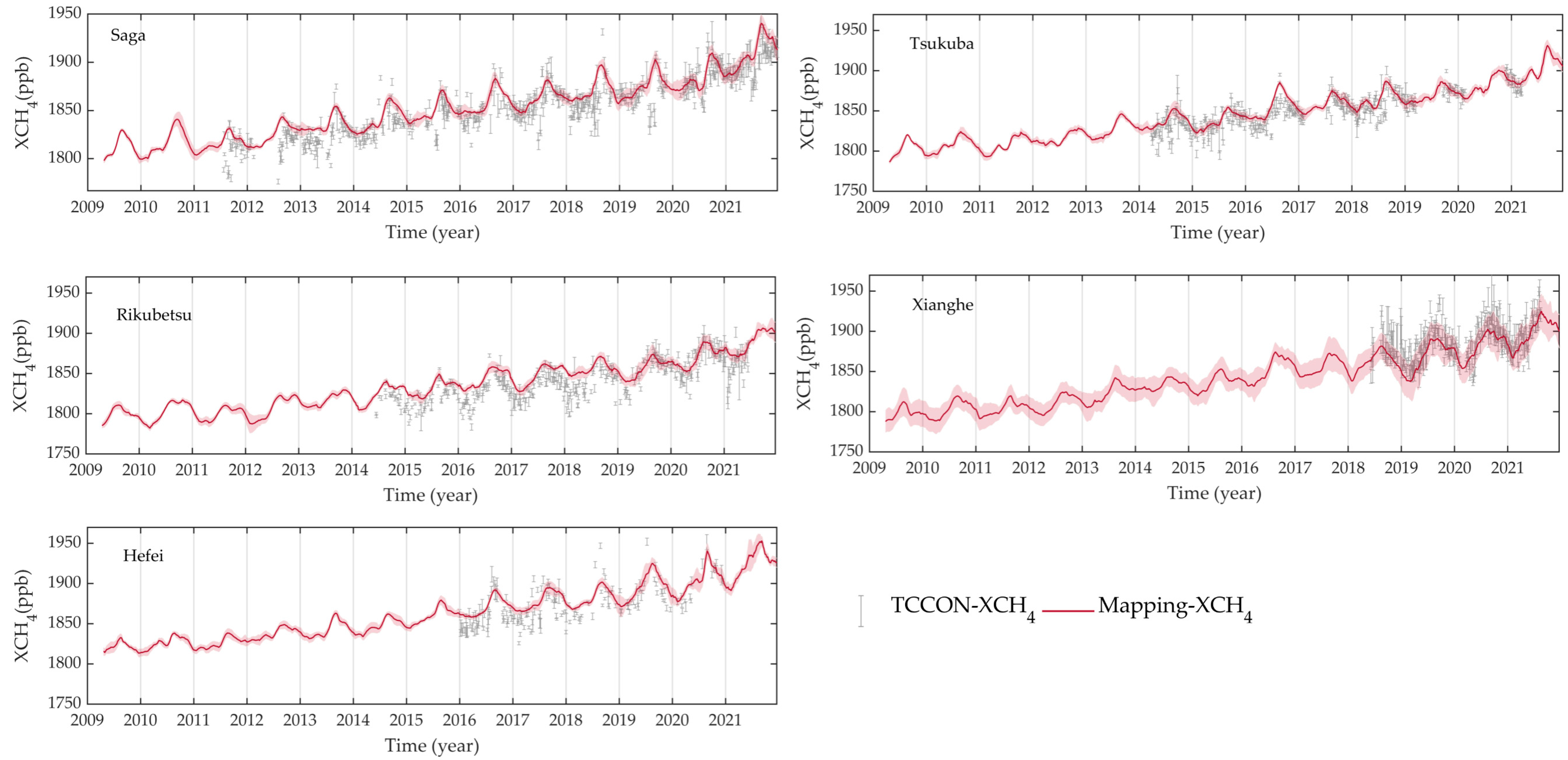
2.1.2. Ground-Based XCH4 Data
2.1.3. CH4 Emission Data from EDGAR
2.2. Methods
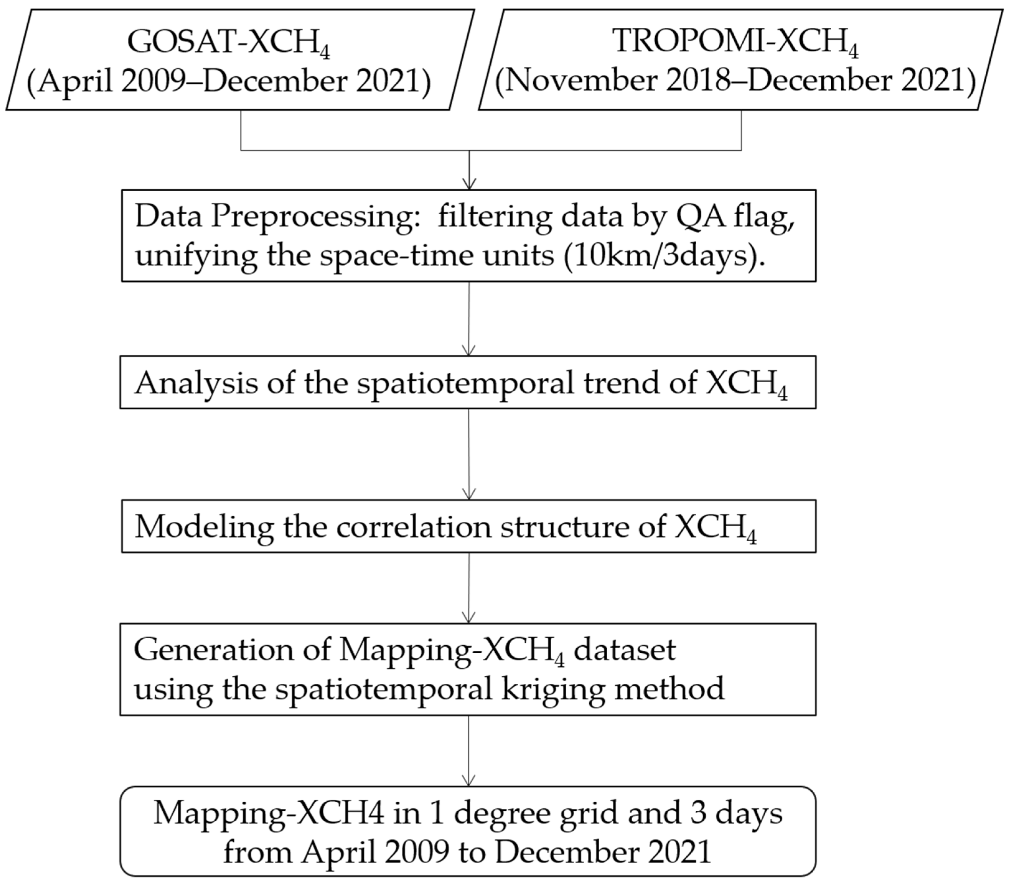
2.2.1. The XCH4 Mapping Method Using GOSAT and TROPOMI Observations
- (1)
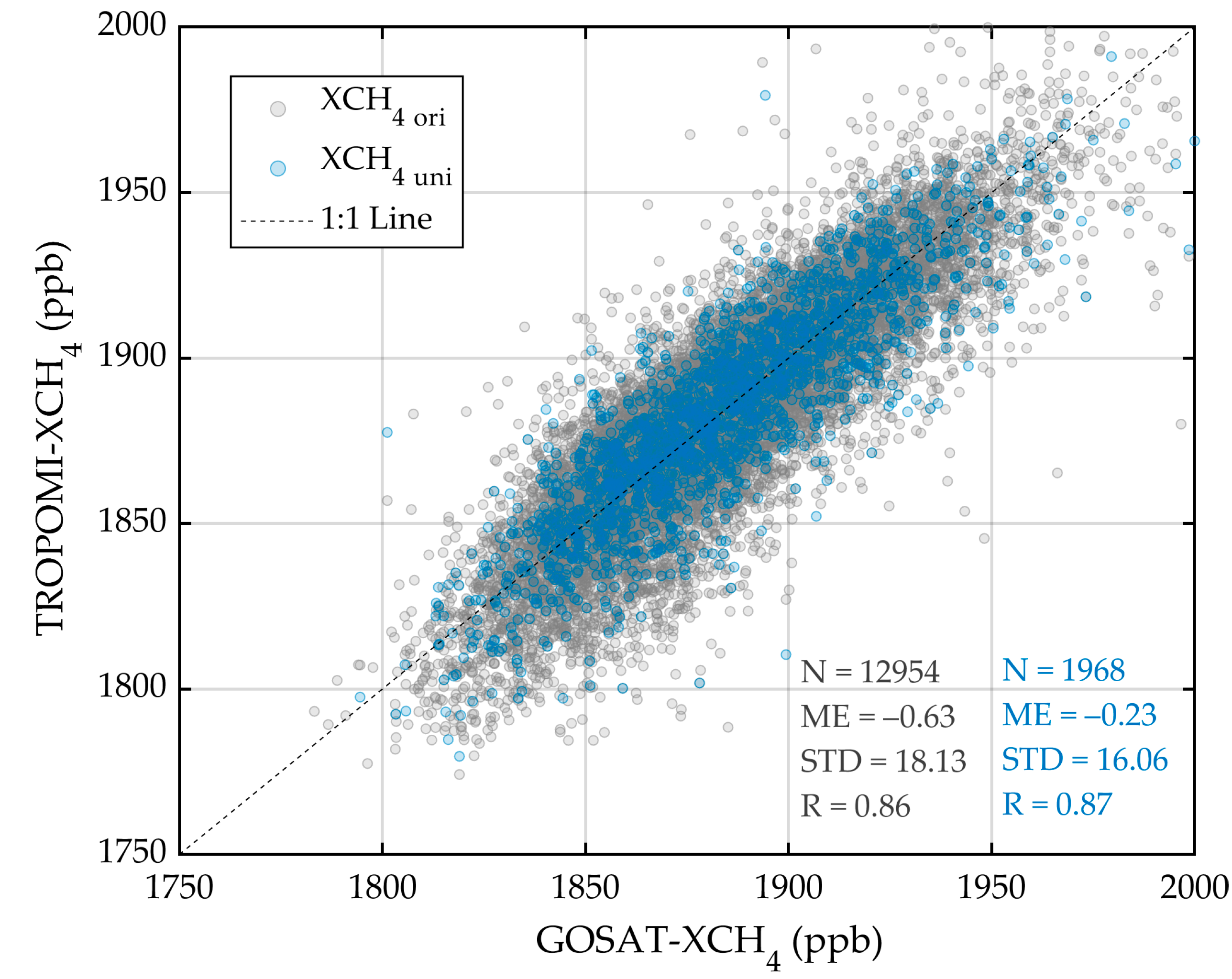
- Data preprocessing
- (2)
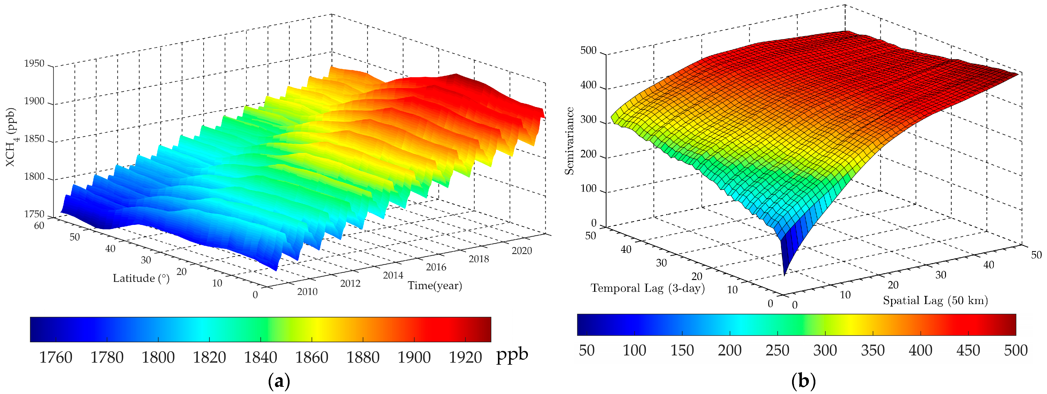
- Spatiotemporal correlation analysis
- (3)
- The mapping of gridded XCH4 data
2.2.2. Local Indicators of Spatial Association
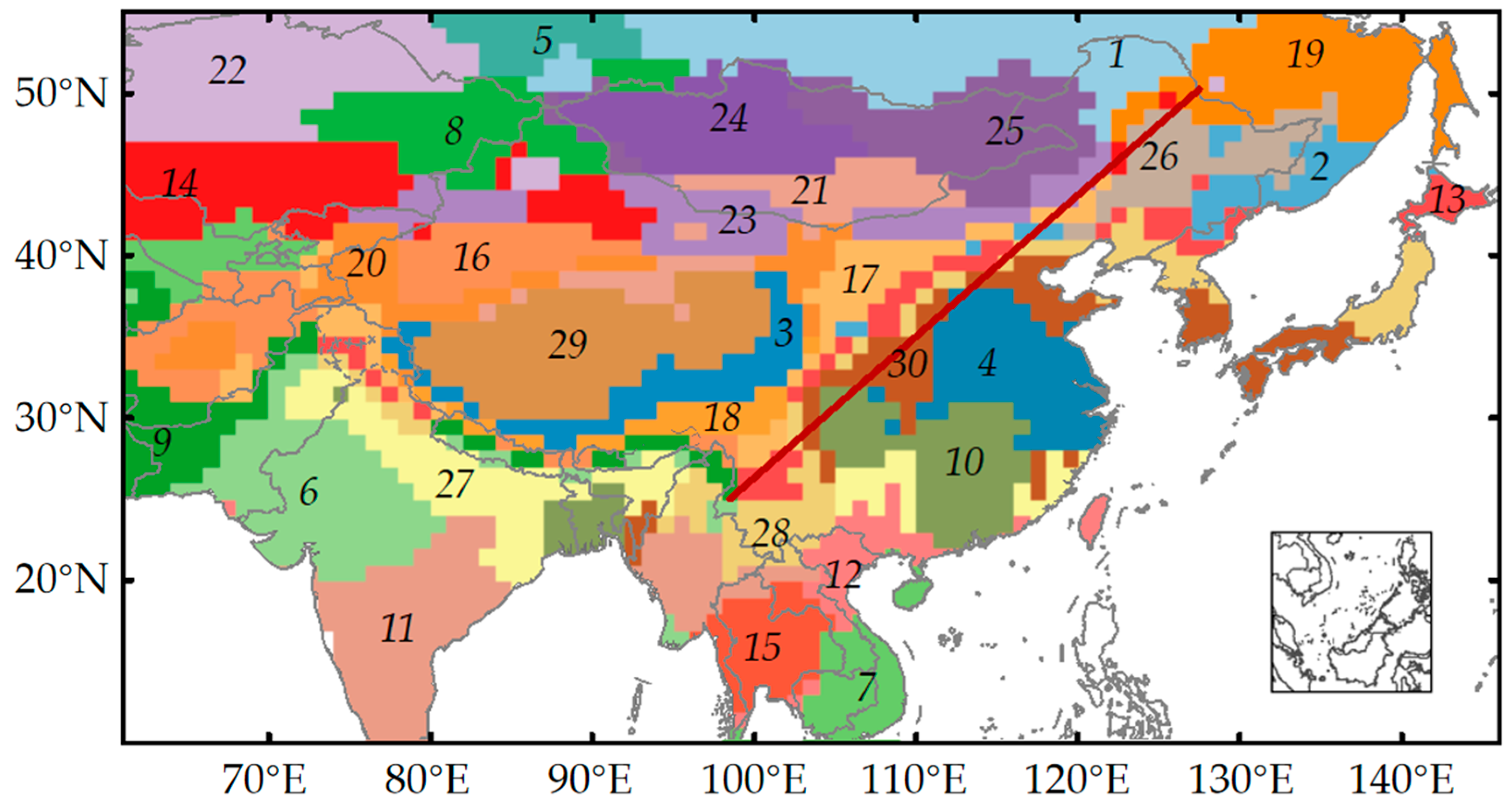
2.2.3. Clustering Spatial Pattern of XCH4 Temporal Changes
3. Results
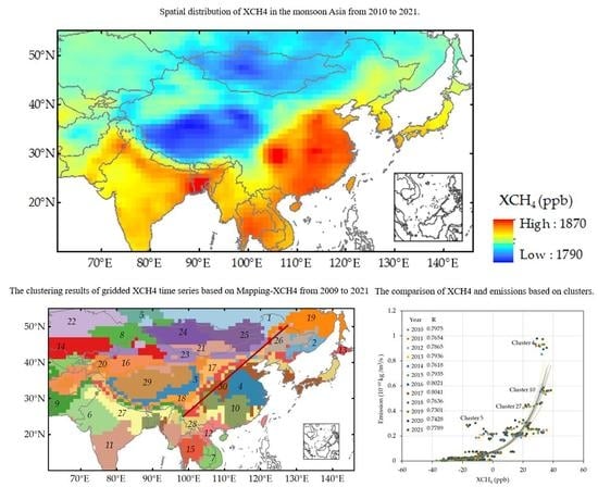
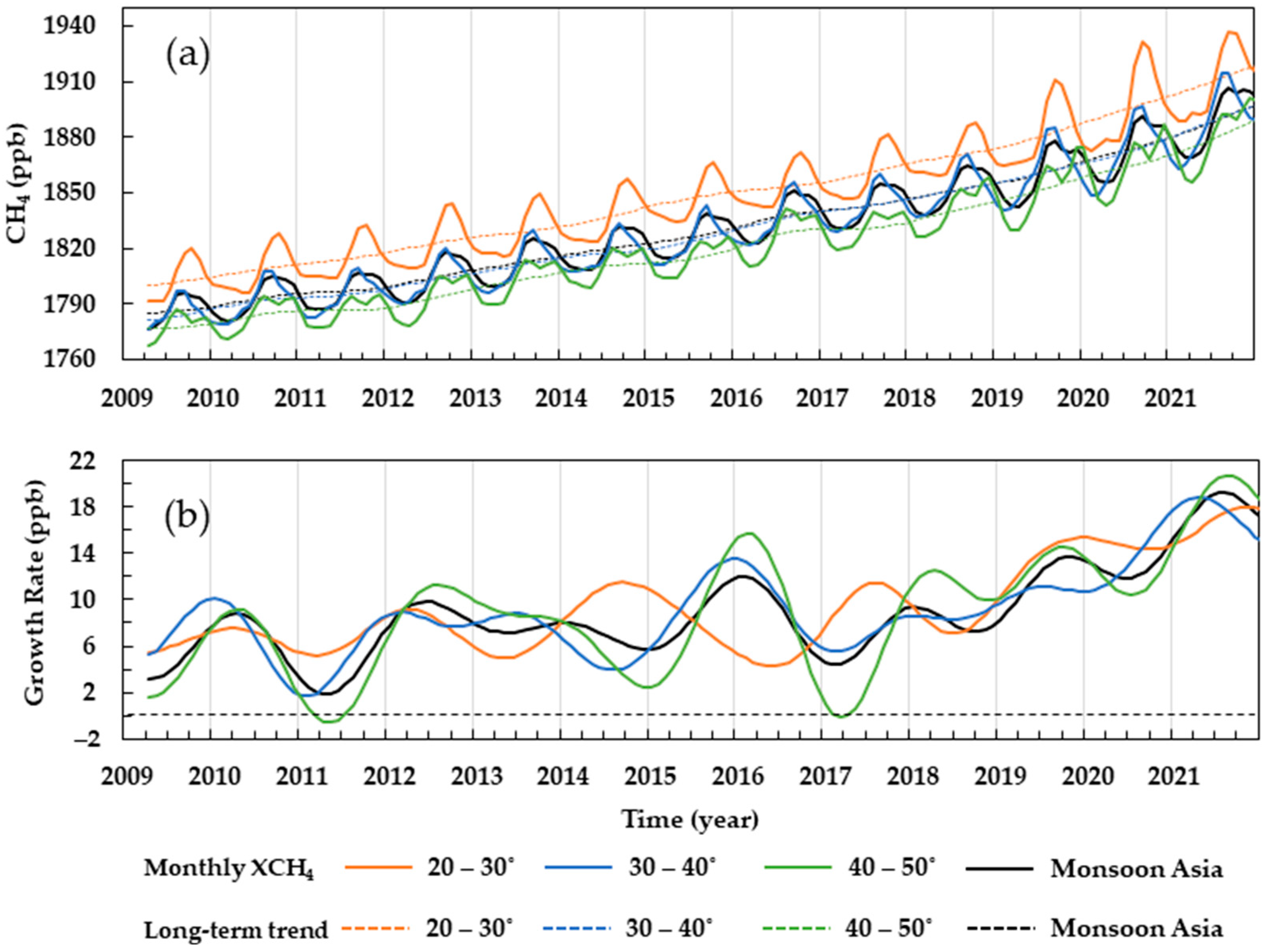
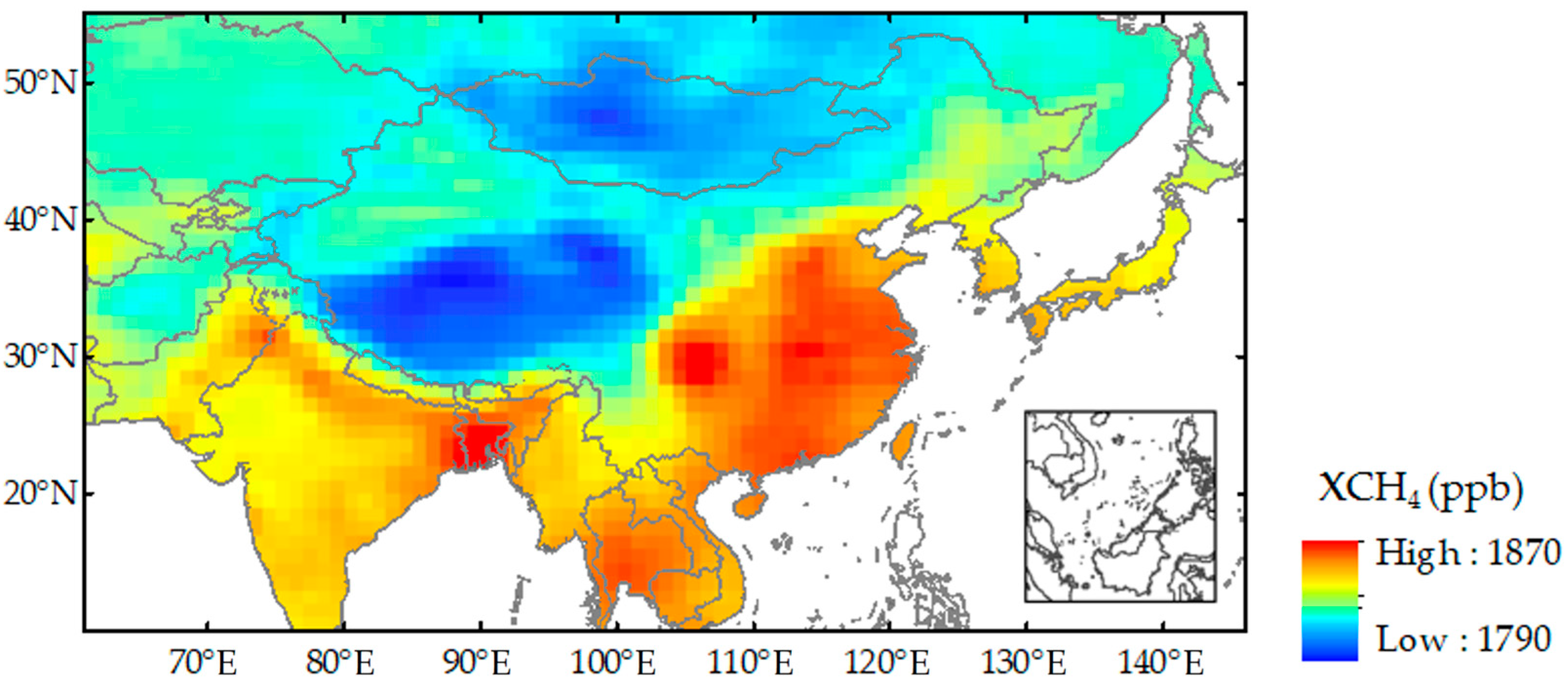
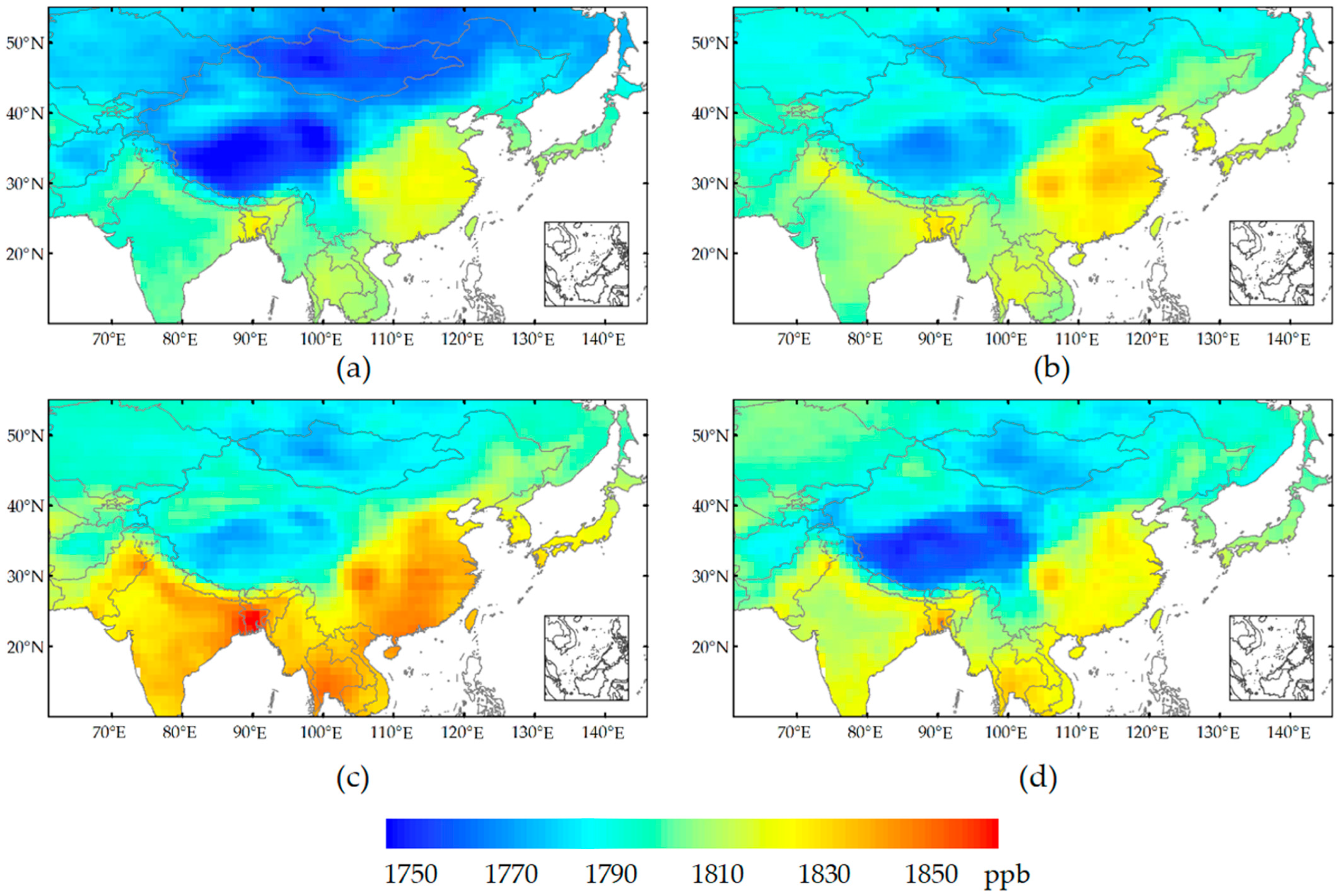
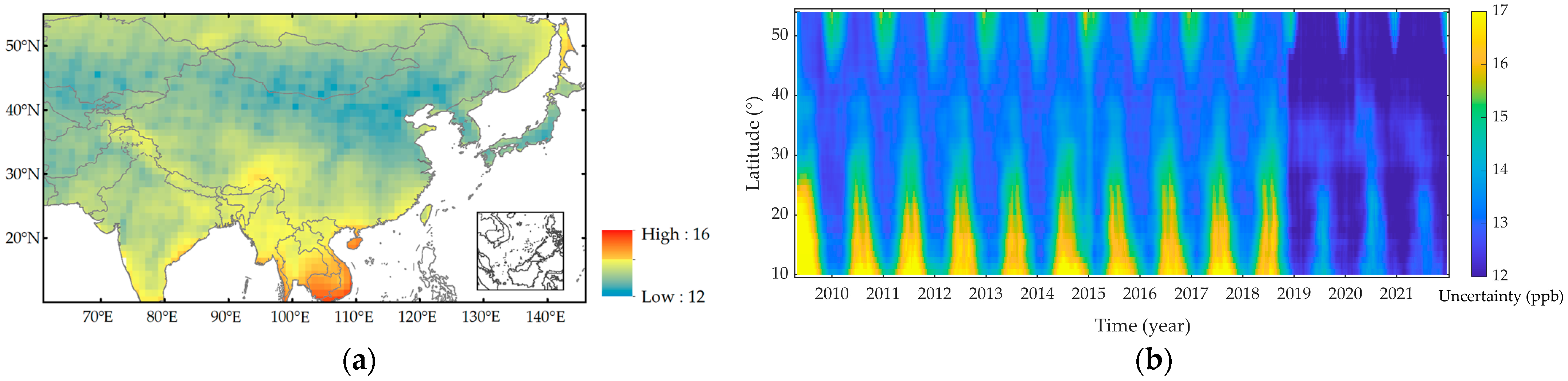
3.1. Spatiotemporal Characteristic of XCH4 Variations in the Asian Monsoon Region from 2009 to 2021
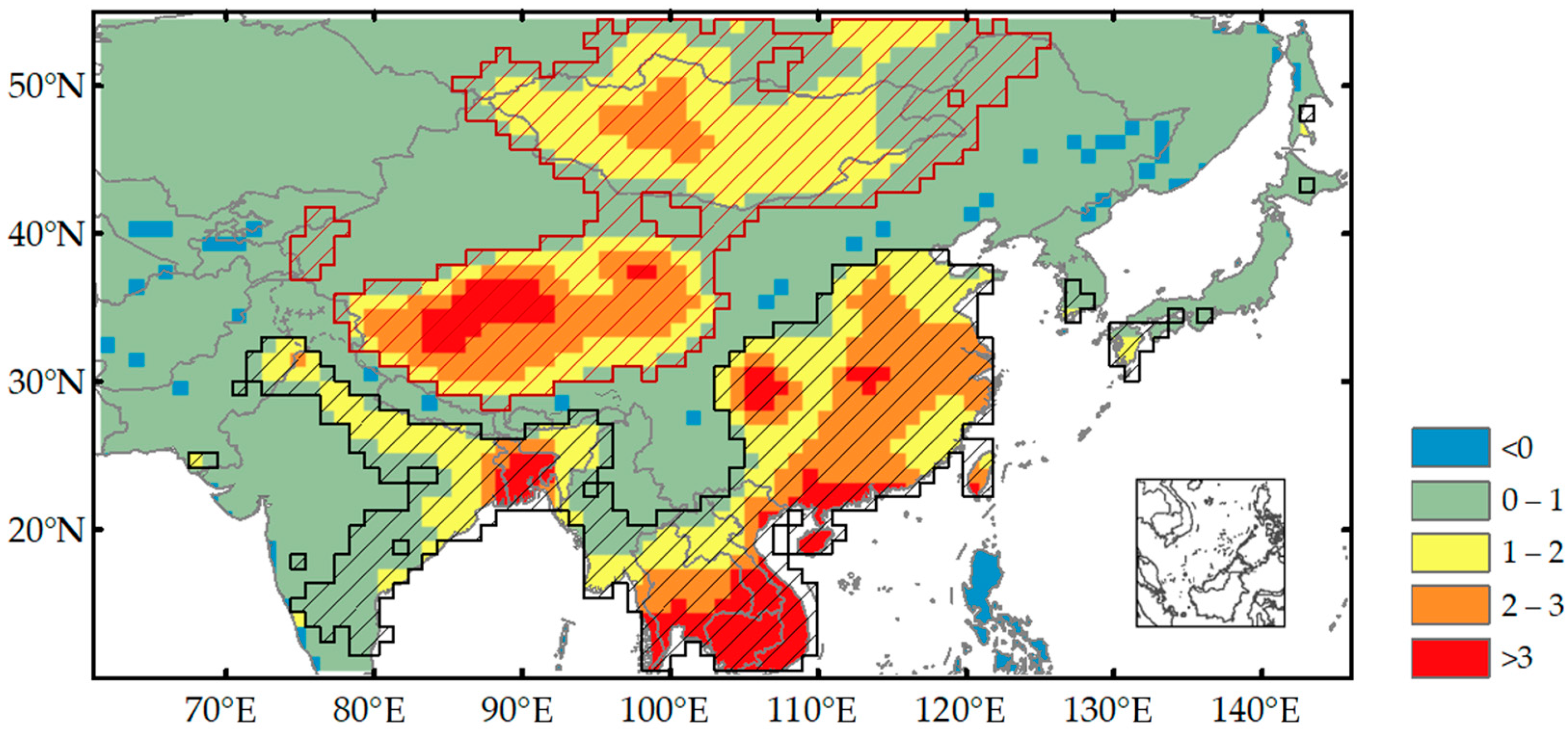
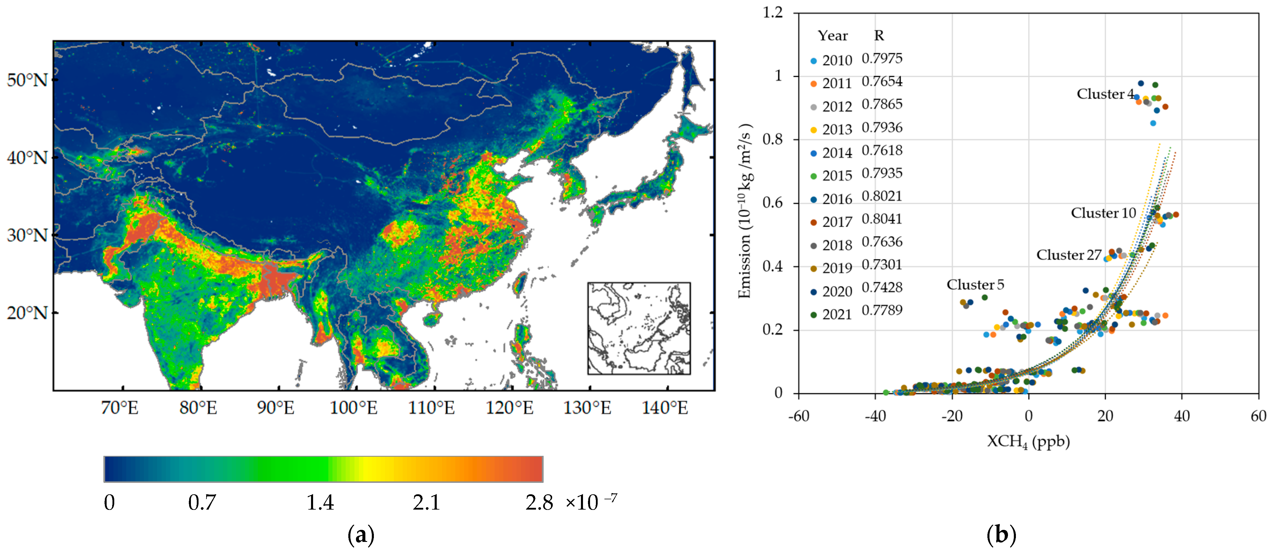
3.2. Spatial Pattern of XCH4 Variations Corresponding to the Surface Emissions
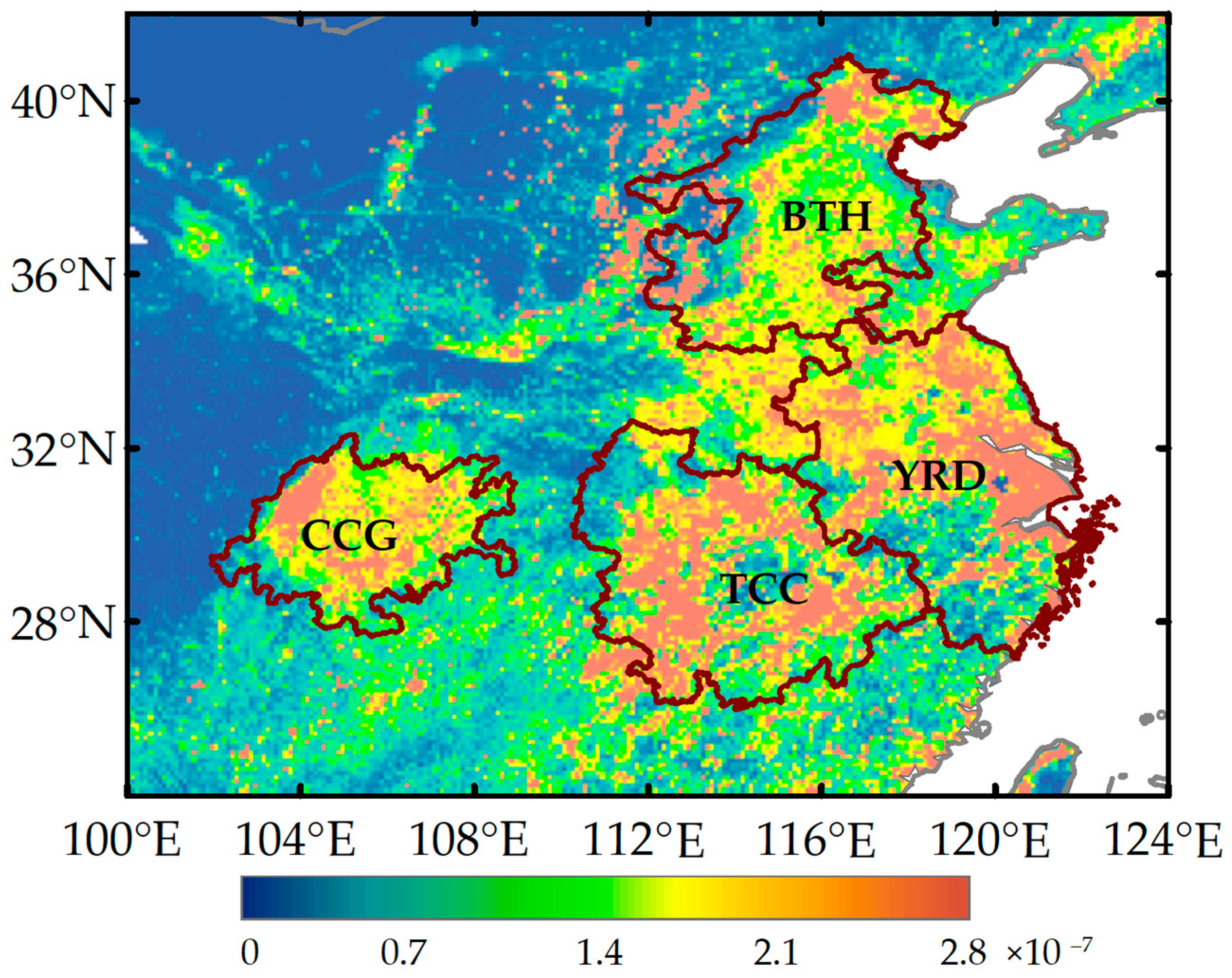
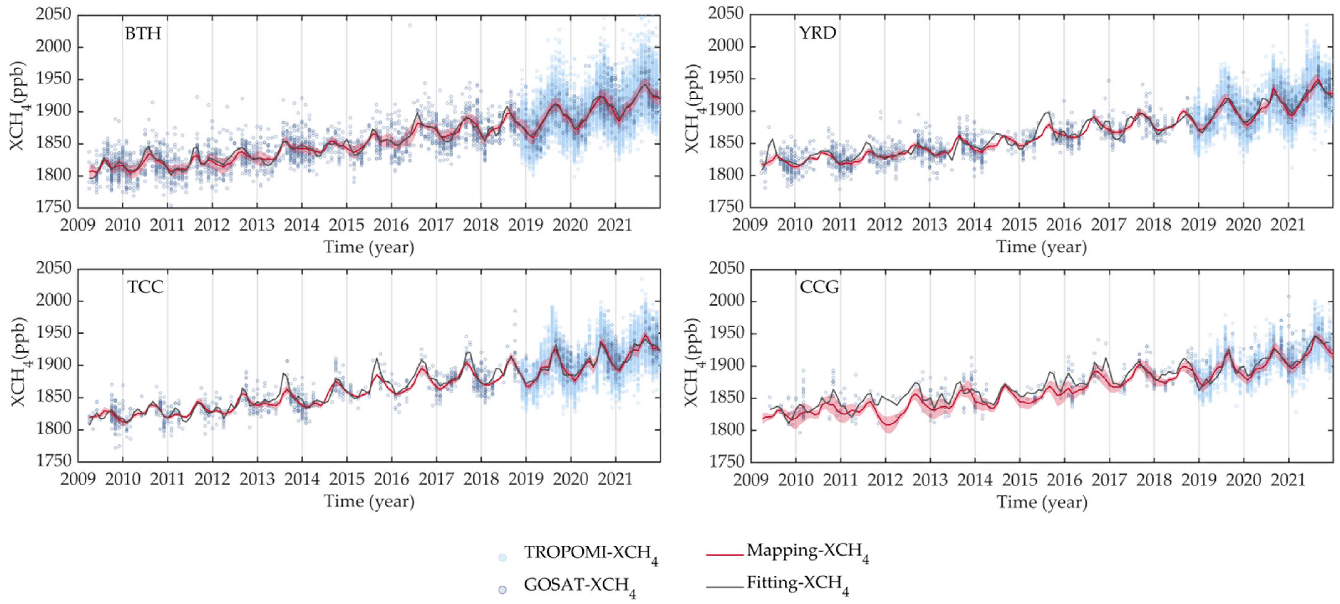
3.3. Regional Characteristics of XCH4 Variations in Urban Agglomerations of China
4. Discussion
5. Conclusions
Author Contributions
Funding
Data Availability Statement
Acknowledgments
Conflicts of Interest
References
- Lin, X.; Zhang, W.; Crippa, M.; Peng, S.; Han, P.; Zeng, N.; Yu, L.; Wang, G. A Comparative Study of Anthropogenic CH4 Emissions over China Based on the Ensembles of Bottom-up Inventories. Earth Syst. Sci. Data 2021, 13, 1073–1088. [Google Scholar] [CrossRef]
- Shukla, P.R.; Skea, J.; Slade, R.; Al Khourdajie, A.; Van Diemen, R.; McCollum, D.; Pathak, M.; Some, S.; Vyas, P.; Fradera, R. IPCC, 2022: Climate Change 2022: Mitigation of Climate Change. Contribution of Working Group III to the Sixth Assessment Report of the Intergovernmental Panel on Climate Change; Cambridge University Press: Cambridge, UK; New York, NY, USA, 2022; Volume 10, p. 9781009157926. [Google Scholar]
- Nisbet, E.G.; Manning, M.R.; Dlugokencky, E.J.; Fisher, R.E.; Lowry, D.; Michel, S.E.; Myhre, C.L.; Platt, S.M.; Allen, G.; Bousquet, P.; et al. Very Strong Atmospheric Methane Growth in the 4 Years 2014–2017: Implications for the Paris Agreement. Glob. Biogeochem. Cycles 2019, 33, 318–342. [Google Scholar] [CrossRef] [Green Version]
- Wuebbles, D.J.; Hayhoe, K.A.; Kotamarthi, R. Methane in the Global Environment. Atmos. Methane Its Role Glob. Environ. 2000, 12, 304–341. [Google Scholar]
- World Meteorological Organization (WMO). Greenhouse Gas Bulletin (GHG Bulletin): The State of Greenhouse Gases in the Atmosphere Based on Global Observations through 2021 (No. 18|26 October 2022); WMO: Geneva, Switzerland, 2022. [Google Scholar]
- Bruhwiler, L.; Dlugokencky, E.; Masarie, K.; Ishizawa, M.; Andrews, A.; Miller, J.; Sweeney, C.; Tans, P.; Worthy, D. CarbonTracker-CH 4: An Assimilation System for Estimating Emissions of Atmospheric Methane. Atmos. Chem. Phys. 2014, 14, 8269–8293. [Google Scholar] [CrossRef] [Green Version]
- Menon, S.; Denman, K.L.; Brasseur, G.; Chidthaisong, A.; Ciais, P.; Cox, P.M.; Dickinson, R.E.; Hauglustaine, D.; Heinze, C.; Holland, E.; et al. Couplings between Changes in the Climate System and Biogeochemistry; Lawrence Berkeley National Lab: Berkeley, CA, USA, 2007. [Google Scholar]
- Zhang, B.; Yang, T.R.; Chen, B.; Sun, X.D. China’s Regional CH4 Emissions: Characteristics, Interregional Transfer and Mitigation Policies. Appl. Energy 2016, 184, 1184–1195. [Google Scholar] [CrossRef]
- Dlugokencky, E.J.; Nisbet, E.G.; Fisher, R.; Lowry, D. Global Atmospheric Methane: Budget, Changes and Dangers. Philos. Trans. R. Soc. Math. Phys. Eng. Sci. 2011, 369, 2058–2072. [Google Scholar] [CrossRef] [Green Version]
- Shi, T.; Han, G.; Ma, X.; Mao, H.; Chen, C.; Han, Z.; Pei, Z.; Zhang, H.; Li, S.; Gong, W. Quantifying Factory-Scale CO2/CH4 Emission Based on Mobile Measurements and EMISSION-PARTITION Model: Cases in China. Environ. Res. Lett. 2023, 18, 034028. [Google Scholar] [CrossRef]
- World Meteorological Organization (WMO). Greenhouse Gas Bulletin (GHG Bulletin)-No. 14: The State of Greenhouse Gases in the Atmosphere Based on Global Observations through 2017; WMO: Geneva, Switzerland, 2017. [Google Scholar]
- Jackson, R.B.; Saunois, M.; Bousquet, P.; Canadell, J.G.; Poulter, B.; Stavert, A.R.; Bergamaschi, P.; Niwa, Y.; Segers, A.; Tsuruta, A. Increasing Anthropogenic Methane Emissions Arise Equally from Agricultural and Fossil Fuel Sources. Environ. Res. Lett. 2020, 15, 071002. [Google Scholar] [CrossRef]
- Sheng, M.; Lei, L.; Zeng, Z.-C.; Rao, W.; Zhang, S. Detecting the Responses of CO2 Column Abundances to Anthropogenic Emissions from Satellite Observations of GOSAT and OCO-2. Remote Sens. 2021, 13, 3524. [Google Scholar] [CrossRef]
- Zeng, Z.; Lei, L.; Hou, S.; Ru, F.; Guan, X.; Zhang, B. A Regional Gap-Filling Method Based on Spatiotemporal Variogram Model of CO2 Columns. IEEE Trans. Geosci. Remote Sens. 2013, 52, 3594–3603. [Google Scholar] [CrossRef]
- Xu, J.; Li, W.; Xie, H.; Wang, Y.; Wang, L.; Hu, F. Long-Term Trends and Spatiotemporal Variations in Atmospheric XCH4 over China Utilizing Satellite Observations. Atmosphere 2022, 13, 525. [Google Scholar] [CrossRef]
- Tomosada, M.; Kanefuji, K.; Matsumoto, Y.; Tsubaki, H. A Prediction Method of the Global Distribution Map of CO2 Column Abundance Retrieved from GOSAT Observation Derived from Ordinary Kriging. In Proceedings of the 2009 ICCAS-SICE, Fukuoka, Japan, 18–21 August 2009; IEEE: Scottsdale, AZ, USA, 2009; pp. 4869–4873. [Google Scholar]
- Liu, Y.; Wang, X.; Guo, M.; Tani, H. Mapping the FTS SWIR L2 Product of XCO2 and XCH4 Data from the GOSAT by the Kriging Method–a Case Study in East Asia. Int. J. Remote Sens. 2012, 33, 3004–3025. [Google Scholar] [CrossRef] [Green Version]
- Liu, M.; Lei, L.; Liu, D.; Zeng, Z.-C. Geostatistical Analysis of CH4 Columns over Monsoon Asia Using Five Years of GOSAT Observations. Remote Sens. 2016, 8, 361. [Google Scholar] [CrossRef] [Green Version]
- Li, L.; Lei, L.; Song, H.; Zeng, Z.; He, Z. Spatiotemporal Geostatistical Analysis and Global Mapping of CH4 Columns from GOSAT Observations. Remote Sens. 2022, 14, 654. [Google Scholar] [CrossRef]
- NIES. GOSAT Project Release Note of Bias-Corrected FTS SWIR Level 2 CO2, CH4 Products (V02.95/V02.96) for General Users; Copernicus Publications: Gottingen, Germany, 2021. [Google Scholar]
- Landgraf, J.; Lorente, A.; Borsdorff, T.; Hasekamp, O.P.; de Gouw, J.; Veefkind, P. Two Year of TROPOMI Methane Observations: Data Quality and Science Opportunities. In Proceedings of the AGU Fall Meeting Abstracts, San Francisco, CA, USA, 9–13 December 2019; Volume 2019, p. A53F-01. [Google Scholar]
- Lorente, A.; Borsdorff, T.; Butz, A.; Langerock, B.; Sha, M.K.; Hasekamp, O.P.; Landgraf, J. TROPOMI Methane Total Column Measurements from TROPOMI S5-P and Suomi-NPP: Improved Data Quality, Validation and First Applications. In Proceedings of the AGU Fall Meeting Abstracts, San Francisco, CA, USA, 9–13 December 2019; Volume 2019, p. A43J-2974. [Google Scholar]
- Sha, M.K.; Langerock, B.; Blavier, J.-F.L.; Blumenstock, T.; Borsdorff, T.; Buschmann, M.; Dehn, A.; De Mazière, M.; Deutscher, N.M.; Feist, D.G.; et al. Validation of Methane and Carbon Monoxide from Sentinel-5 Precursor Using TCCON and NDACC-IRWG Stations. Atmos. Meas. Technol. 2021, 14, 6249–6304. [Google Scholar] [CrossRef]
- Shiomi, K.; Kawakami, S.; Ohyama, H.; Arai, K.; Okumura, H.; Ikegami, H.; Usami, M. GGG2020.R0, TCCON Data from Saga (JP); Caltech Library: Pasadena, CA, USA, 2022. [Google Scholar] [CrossRef]
- Morino, I.; Ohyama, H.; Hori, A.; Ikegami, H. GGG2020.R0, TCCON Data from Rikubetsu (JP); Caltech Library: Pasadena, CA, USA, 2022. [Google Scholar] [CrossRef]
- Morino, I.; Ohyama, H.; Hori, A.; Ikegami, H. GGG2020.R0, TCCON Data from Tsukuba (JP), 125HR; Caltech Library: Pasadena, CA, USA, 2022. [Google Scholar] [CrossRef]
- Zhou, M.; Wang, P.; Kumps, N.; Hermans, C.; Nan, W. GGG2020.R0, TCCON Data from Xianghe, China; Caltech Library: Pasadena, CA, USA, 2022. [Google Scholar] [CrossRef]
- Liu, C.; Wang, W.; Sun, Y.; Shan, C. GGG2020.R0, TCCON Data from Hefei (PRC); Caltech Library: Pasadena, CA, USA, 2022. [Google Scholar] [CrossRef]
- Crippa, M.; Solazzo, E.; Huang, G.; Guizzardi, D.; Koffi, E.; Muntean, M.; Schieberle, C.; Friedrich, R.; Janssens-Maenhout, G. High Resolution Temporal Profiles in the Emissions Database for Global Atmospheric Research. Sci. Data 2020, 7, 121. [Google Scholar] [CrossRef] [Green Version]
- Muntean, M.; Janssens-Maenhout, G.; Song, S.; Giang, A.; Selin, N.E.; Zhong, H.; Zhao, Y.; Olivier, J.G.J.; Guizzardi, D.; Crippa, M.; et al. Evaluating EDGARv4.Tox2 Speciated Mercury Emissions Ex-Post Scenarios and Their Impacts on Modelled Global and Regional Wet Deposition Patterns. Atmos. Environ. 2018, 184, 56–68. [Google Scholar] [CrossRef]
- Han, P.; Zeng, N.; Oda, T.; Lin, X.; Crippa, M.; Guan, D.; Janssens-Maenhout, G.; Ma, X.; Liu, Z.; Shan, Y.; et al. Evaluating China’s Fossil-Fuel CO2 Emissions from a Comprehensive Dataset of Nine Inventories. Atmos. Chem. Phys. 2020, 20, 11371–11385. [Google Scholar] [CrossRef]
- Crippa, M.; Guizzardi, D.; Solazzo, E.; Muntean, M.; Schaaf, E.; Monforti-Ferrario, F.; Banja, M.; Olivier, J.; Grassi, G.; Rossi, S. GHG Emissions of All World Countries; Publications Office of the European Union: Luxembourg, 2021. [Google Scholar]
- Zeng, Z.-C.; Lei, L.; Strong, K.; Jones, D.B.; Guo, L.; Liu, M.; Deng, F.; Deutscher, N.M.; Dubey, M.K.; Griffith, D.W. Global Land Mapping of Satellite-Observed CO2 Total Columns Using Spatio-Temporal Geostatistics. Int. J. Digit. Earth 2017, 10, 426–456. [Google Scholar] [CrossRef] [Green Version]
- He, Z.; Lei, L.; Zhang, Y.; Sheng, M.; Wu, C.; Li, L.; Zeng, Z.-C.; Welp, L.R. Spatio-Temporal Mapping of Multi-Satellite Observed Column Atmospheric CO2 Using Precision-Weighted Kriging Method. Remote Sens. 2020, 12, 576. [Google Scholar] [CrossRef] [Green Version]
- Anselin, L. Local Indicators of Spatial Association—LISA. Geogr. Anal. 1995, 27, 93–115. [Google Scholar] [CrossRef]
- Bivand, R.S.; Wong, D.W. Comparing Implementations of Global and Local Indicators of Spatial Association. Test 2018, 27, 716–748. [Google Scholar] [CrossRef]
- Kennedy, J.; Eberhart, R. Particle Swarm Optimization. In Proceedings of the IEEE ICNN’95-International Conference on Neural Networks, Perth, WA, USA, 27 November–1 December 1995; Volume 4, pp. 1942–1948. [Google Scholar]
- Mucherino, A.; Papajorgji, P.J.; Pardalos, P.M.; Mucherino, A.; Papajorgji, P.J.; Pardalos, P.M. K-Nearest Neighbor Classification. Data Min. Agric. 2009, 34, 83–106. [Google Scholar]
- Huang, L.; Ning, Z.; Lin, H.; Zhou, W.; Wang, L.; Zou, J.; Xu, H. High-Pressure Sorption of Methane, Ethane, and Their Mixtures on Shales from Sichuan Basin, China. Energy Fuels 2021, 35, 3989–3999. [Google Scholar] [CrossRef]
- Song, K.; Zhang, G.; Yu, H.; Xu, H.; Lv, S.; Ma, J. Methane and Nitrous Oxide Emissions from a Ratoon Paddy Field in Sichuan Province, China. Eur. J. Soil Sci. 2021, 72, 1478–1491. [Google Scholar] [CrossRef]
- Behera, M.D.; Mudi, S.; Shome, P.; Das, P.K.; Kumar, S.; Joshi, A.; Rathore, A.; Deep, A.; Kumar, A.; Sanwariya, C. COVID-19 Slowdown Induced Improvement in Air Quality in India: Rapid Assessment Using Sentinel-5P TROPOMI Data. Geocarto Int. 2021, 37, 8127–8147. [Google Scholar] [CrossRef]
- Gupta, K.; Kumar, R.; Baruah, K.K.; Hazarika, S.; Karmakar, S.; Bordoloi, N. Greenhouse Gas Emission from Rice Fields: A Review from Indian Context. Environ. Sci. Pollut. Res. 2021, 28, 30551–30572. [Google Scholar] [CrossRef]
- Metya, A.; Datye, A.; Chakraborty, S.; Tiwari, Y.K.; Sarma, D.; Bora, A.; Gogoi, N. Diurnal and Seasonal Variability of CO2 and CH4 Concentration in a Semi-Urban Environment of Western India. Sci. Rep. 2021, 11, 2931. [Google Scholar] [CrossRef]
- Wu, D.; Lin, J.C.; Fasoli, B.; Oda, T.; Ye, X.; Lauvaux, T.; Yang, E.G.; Kort, E.A. A Lagrangian Approach towards Extracting Signals of Urban CO2 Emissions from Satellite Observations of Atmospheric Column CO2 (XCO2): X-Stochastic Time-Inverted Lagrangian Transport Model (“X-STILT V1”). Geosci. Model Dev. 2018, 11, 4843–4871. [Google Scholar] [CrossRef] [Green Version]
- Belikov, D.A.; Saitoh, N.; Patra, P.K.; Chandra, N. GOSAT CH4 Vertical Profiles over the Indian Subcontinent: Effect of a Priori and Averaging Kernels for Climate Applications. Remote Sens. 2021, 13, 1677. [Google Scholar] [CrossRef]
- Sheng, M.; Lei, L.; Zeng, Z.-C.; Rao, W.; Song, H.; Wu, C. Global Land 1° Mapping Dataset of XCO 2 from Satellite Observations of GOSAT and OCO-2 from 2009 to 2020. Big Earth Data 2022, 7, 170–190. [Google Scholar] [CrossRef]


| Dataset | GOSAT-XCH4 | TROPOMI-XCH4 |
|---|---|---|
| Period | April 2009–December 2021. | November 2018–December 2021 |
| Data Product | Bias-corrected FTS SWIR L2 CH4 | S5P_OFFL_L2__CH4 |
| Spatiotemporal Resolution | 3 days, 10.5 km | 1 day, ~7 km |
| Criteria of Data Screening | xCH4_quality_flag = 0, land_fraction > 90 | qa_value > 0.75 |
| Data Source | GDAS | Copernicus S5p Open Access Hub |
| Site | Latitude | Longitude | Start Time | End Time | N | ME | MAE | STD | R |
|---|---|---|---|---|---|---|---|---|---|
| Saga | 33.24°N | 130.29°E | 28 July 2011 | 30 June 2021 | 747 | 8.0386 | 11.3856 | 13.3502 | 0.8970 |
| Rikubetsu | 43.46°N | 143.77°E | 24 June 2014 | 30 June 2021 | 439 | 10.8249 | 13.2031 | 12.7522 | 0.8516 |
| Tsukuba | 36.05°N | 140.12°E | 28 March 2014 | 28 June 2021 | 484 | 5.5391 | 9.0189 | 10.8386 | 0.8452 |
| Xianghe | 39.8°N | 116.96°E | 14 June 2018 | 30 November 2021 | 324 | –9.3133 | 13.8883 | 15.3010 | 0.7261 |
| Hefei | 31.9°N | 119.17°E | 8 January 2016 | 31 December 2020 | 185 | 8.4948 | 13.3280 | 13.7827 | 0.8256 |
Disclaimer/Publisher’s Note: The statements, opinions and data contained in all publications are solely those of the individual author(s) and contributor(s) and not of MDPI and/or the editor(s). MDPI and/or the editor(s) disclaim responsibility for any injury to people or property resulting from any ideas, methods, instructions or products referred to in the content. |
© 2023 by the authors. Licensee MDPI, Basel, Switzerland. This article is an open access article distributed under the terms and conditions of the Creative Commons Attribution (CC BY) license (https://creativecommons.org/licenses/by/4.0/).
Share and Cite
Song, H.; Sheng, M.; Lei, L.; Guo, K.; Zhang, S.; Ji, Z. Spatial and Temporal Variations of Atmospheric CH4 in Monsoon Asia Detected by Satellite Observations of GOSAT and TROPOMI. Remote Sens. 2023, 15, 3389. https://doi.org/10.3390/rs15133389
Song H, Sheng M, Lei L, Guo K, Zhang S, Ji Z. Spatial and Temporal Variations of Atmospheric CH4 in Monsoon Asia Detected by Satellite Observations of GOSAT and TROPOMI. Remote Sensing. 2023; 15(13):3389. https://doi.org/10.3390/rs15133389
Chicago/Turabian StyleSong, Hao, Mengya Sheng, Liping Lei, Kaiyuan Guo, Shaoqing Zhang, and Zhanghui Ji. 2023. "Spatial and Temporal Variations of Atmospheric CH4 in Monsoon Asia Detected by Satellite Observations of GOSAT and TROPOMI" Remote Sensing 15, no. 13: 3389. https://doi.org/10.3390/rs15133389
APA StyleSong, H., Sheng, M., Lei, L., Guo, K., Zhang, S., & Ji, Z. (2023). Spatial and Temporal Variations of Atmospheric CH4 in Monsoon Asia Detected by Satellite Observations of GOSAT and TROPOMI. Remote Sensing, 15(13), 3389. https://doi.org/10.3390/rs15133389