Abstract
The accuracy of surface reflectance estimation for satellite sensors using radiance-based calibrations can depend significantly on the choice of solar spectral irradiance (or solar spectrum) model used for atmospheric correction. Selecting an accurate solar spectrum model is also important for radiance-based sensor calibration and estimation of atmospheric parameters from irradiance observations. Previous research showed that Landsat 8 could be used to evaluate the quality of solar spectrum models. This paper applies the analysis using five previously evaluated and three more recent solar spectrum models using both Landsat 8 (OLI) and Landsat 9 (OLI2). The study was further extended down to 10 nm resolution and a wavelength range from Ultraviolet A (UVA) to shortwave infrared (SWIR) (370–2480 nm) using inversion of field irradiance measurements. The results using OLI and OLI2 as well as the inversion of irradiance measurements were that the more recent Chance and Kurucz (SA2010), Meftah (SOLAR-ISS) and Coddington (TSIS-1) models performed better than all of the previous models. The results were illustrated by simulating dark and bright surface reflectance signatures obtained by atmospheric correction with the different solar spectrum models. The results showed that if the SA2010 model is assumed to be the “true” solar irradiance, using the TSIS-1 or the SOLAR-ISS model will not significantly change the estimated ground reflectance. The other models differ (some to a large extent) in varying wavelength areas.
1. Introduction
An accurate normalized solar spectral irradiance model at the top of the atmosphere (TOA) is very important for atmospheric correction and sensor calibration of Earth observation data [1]. It is also an important boundary condition used in computing the energy balance, heating and cooling of the atmosphere [2] and total solar radiation estimation and is a key factor in models used to invert irradiance data for atmospheric parameters and field estimation of reflectance. Li et al. [3] showed how different choices of the solar spectral irradiance model at mean Sun–Earth distance (in this paper simply called the solar spectrum), at environmental satellite spectral resolution, can significantly impact the surface reflectance retrieval from satellite sensors measuring only calibrated top-of-atmosphere radiance. The findings took advantage of the Landsat 8 Operational Land Imager (OLI) instrument recording both lamp-calibrated radiance data and diffuser panel (or solar diffuser)-referenced reflectance data [4]. If the calibrations for both TOA reflectance and radiance are perfect, these data together can be used to estimate the solar spectrum for the Landsat bands. The analysis in [3] consequently used the observed solar spectrum of Landsat 8 as an estimate of the “true” solar spectrum within the current level of calibration error, where “true” means a hypothetical very accurate estimate. In [3], some suggestions were made as to which solar spectrum selections were “good” or even “best” using the observed Landsat solar spectrum. However, as the Landsat bands are broadband and only cover a few areas of the spectrum, they concluded that it would be best if any revisions were made by groups using recent satellite-based observations to study the solar spectrum at fine spectral resolution.
Since [3] were published, a number of circumstances have led the authors to extend the study and introduce some new methods. Firstly, three additional solar spectrum models may be worth further investigation. One is the Chance and Kurucz (2010) model [5]. This is a significant revision of the Kurucz (2005) [6] model evaluated in [3], although it has only been made available for the UVA-NIR (near infrared) range. Another is the Meftah et al. (2020) update of the SOLAR-ISS model [7], and the third is the recent publication of the Total and Spectral Solar Irradiance Sensor (TSIS-1) spectrum by Coddington et al. (2021) [8]. This has been accepted by the Committee on Earth Observation Satellites (CEOS) as an alternative to the Thuillier et al. (2003) SOLSPEC model [9] for atmospheric correction. In addition, Landsat 9, with the OLI2 instrument, has been launched with near identical spectral characteristics and calibration facilities as Landsat 8 (the OLI instrument), providing an independent estimate of a Landsat-based solar spectrum to increase the certainty of the results.
Recently an increasing number of hyperspectral options has been considered among planned remote sensing satellites. One example is the Hyperspectral Infrared Imager (HyspIRI) mission [10] which is designed to cover the spectral range of 380–2510 nm. The European PRISMA [11] and ENMAP [12] sensors have been collecting hyperspectral data for some time. Both have solar diffusers to support calibration (e.g., [13]). The EMIT [14] sensor is now deployed on the International Space Station (ISS). Others are being planned by various groups for calibration and validation support using lower-cost and lower-orbiting small satellites. Many, including the Surface Biology and Geology (SBG) HyspIRI and EMIT sensors, will apparently only have radiance-calibrated instruments, and the smallsats will also have very limited onboard calibration facilities. In these cases, accurate solar spectrum models are crucial for both calibration and atmospheric correction, especially in the UVA (300–400 nm) area. This paper therefore investigates whether the analysis in [3] can also be extended to investigate the potential issues with choice of solar spectrum models in the UVA area, beyond the range of Landsat 8 (OLI instrument) and 9 (OLI2 instrument).
The evaluation in [3] made use of the advantage of Landsat 8 recording both (lamp-based) radiance and panel-based reflectance measurements at the top of the atmosphere. Landsat 9 has the same opportunity. However, the “accuracy” of the solar spectrum in this analysis involves the spectral resolution of the sensor. The Landsat 8 and 9 bands are broad bands with the finest spectral resolution being about 15 nm. Almost all of the missions of interest will collect some or all data with at least a 10 nm or coarser resolution. Therefore, 10 nm has been selected as the base resolution for the extended study.
General studies of solar spectral irradiance have been advanced significantly in recent years by satellite observations such as Solar Radiation and Climate Experiment (SOURCE), the Total Irradiance Monitor (TIM) [15,16], the International Space Station-based SOLAR-ISS [7] and the TSIS-1 [8]. However, the very fine scale resolutions used in these studies are not needed to answer questions of interest to planned Earth observation missions at their currently planned resolutions. These questions include how much variation may occur in estimated surface reflectance due only to the choice of solar spectrum model. It is important to know what the magnitude of the variations may be and which solar spectrum models are most suitable to use at resolutions lower than 5–10 nm.
In this study, the method introduced in [3] is firstly applied to the previous Landsat 8 and then, using the equivalent evaluation, applied to the more recent Landsat 9 data. The study is then further extended to hyperspectral solar spectrum resolutions at 10 nm and to the UVA region using high spectral resolution surface irradiance measurements obtained by field radiometry. The extended study uses inversions of atmospheric parameters with measured irradiance data to separate solar spectra. The separation is based on the changes in parameter estimates and goodness of fit that occur when solar spectra are changed. Final conclusions are made on the combined results of the two analyses.
2. Methods
2.1. Model Evaluation Using Landsat 8 and 9 Solar Spectrum Observations
In [3], the effect of using different solar spectra on surface reflectance was evaluated and modeled to derive an expression for the difference that can occur in an estimated surface reflectance by using a different solar spectrum model. This expression was used in [3] to explain anomalous differences that occurred in atmospheric corrections for the Landsat 8 coastal blue band (band 1) and could not be explained as errors in calibration. Li et al. [3] also proposed a method to evaluate the performance of different solar spectrum models using independent calibrations of both radiance and reflectance available in the Landsat OLI sensor. The models and the implications are described in detail in [3]. In this section, some key equations are briefly presented, as they will be used to analyze the new data.
The solar spectrum term occurs in atmospheric correction for radiance-based observations primarily in the surface irradiance and path radiance. Therefore, a relatively simple atmospheric correction expression based on a Lambertian surface can be used to derive how estimated surface reflectance can change if a different solar spectrum model is used [3]. In the real situation, the surface is not Lambertian; however, most operational land surface reflectance products produce Lambertian surface reflectance. With this assumption, the relationship between the reflectance at the TOA and surface can be written as follows [3]:
Ts and Tv are the total transmittances in the sun and view directions, S is atmospheric albedo, is the TOA reflectance, is effective path reflectance and is related to the surface reflectance as . Without loss of generality, the results can be derived in terms of . If is measured, such as when the sensor uses a reference solar diffuser (sometimes called a panel or a plaque) to directly estimate , this equation is independent of the solar spectrum.
For the radiance-based situation, Ltoa is the measured and calibrated TOA radiance at the sensor and θs is the solar zenith angle. is written for a solar spectrum modified for Sun–Earth distance (indicated by the prime), and then
The TOA estimates for in Equations (1) and (2) should be the same if the solar spectrum is the “true” solar spectrum. If E01 and E02 are two different solar spectra and and are their corresponding Earth–Sun-adjusted values, then the ratio of the TOA reflectance estimates between the two choices of solar spectrum can be written as follows [3]:
For the TOA reflectance based on the solar diffuser on board a satellite, the estimate is made differently. The actual solar spectral irradiance at TOA () is reflected from the solar diffuser to fill the field of view of the instrument. The radiance is measured by each detector. If is the reflectance of the satellite solar diffuser (strictly bidirectional reflectance function (BRF)) then the calibrated solar diffuser radiance () is
The calculation of the TOA reflectance in this case is then (noting that the solar diffuser is assumed normal to the solar radiation)
From Equation (5), there are two outcomes. The first is that the radiance calibrations cancel in the ratio of to , and these can be replaced by the digital numbers of the two measurements. That is, can be computed if is known without any reference to a solar spectrum and with no dependence on a radiance calibration. The second equality shows that Equation (5) is in the same form as Equation (2) with the “true” solar spectrum replacing the selected one.
In Equation (3), if (the measured TOA reflectance of the solar diffuser) then the ratio will be that of the “true” solar spectrum to the selected solar spectrum [3] if the calibration of the sensor is perfect. The relationship between the various selections of the solar spectrum and an estimate for the “true” solar spectrum was established in [3] by considering , which can be seen as a relative error between the selected and estimated “true” solar spectrum using Equation (3):
The Landsat OLI and OLI2 instruments produce both TOA reflectance based on onboard solar diffuser reflectance and independent radiances based on pre-launch and in-orbit lamp readings [4]. Using another choice of the solar spectrum to convert TOA radiance to TOA reflectance allows rt to be estimated by Equation (3). If one of the solar spectra is a very close estimate for the “true” solar spectrum, then Equation (6) implies that a choice of the other solar spectrum is equally good as the estimated “true” one if rt = 1.
Li et al. [3] demonstrated and modeled the consequences of differences between solar spectrum models as expressed in Equation (6). The differences had been observed in Landsat data. According to [3], the relationship between surface reflectance estimated using E02 () and that using E01 () based on Equation (1) directly can be expressed as follows:
In this equation, is a bias term that arises in the blue/green end of the spectrum as the diffuse component increases with the decrease in the wavelength. The details of this derivation can be found in [3] where the model was used to explain the observed effects of using different selections of the solar spectrum in images. The significance of the factors in this equation was most clear when band 1 data were considered.
Defining rs = Equation (7) explains how the change from rt to rs can be highly variable depending on the band (worst in the blue end of the spectrum), atmosphere and land cover. Originally, a problem observed in Landsat 8 images was thought to be due to calibration error, but the types of changes observed at the surface could not be explained as a simple change in calibration gain. Quite small differences in rt can lead to large changes on the ground—especially in the blue bands. In Section 4.4 of this paper, Equation (7) is used to demonstrate the type of changes that may occur due to differences in the selected solar spectrum for darker signatures, such as water, in the UVA to green regions of the spectrum.
If, hypothetically, one of the solar spectra is the “true” solar spectrum, then Equation (7) models the differences between surface reflectance due to the difference between the chosen solar spectrum and the “true” case. If the two selected solar spectra are existing models, calibration errors do not affect the differences found but Equation (7) still holds. However, relative to the “true” solar spectrum, calibration errors can behave as additional (fixed) perturbations. As noted before, because Landsat 8 and 9 have both NIST traceable lamp calibration and a solar diffuser for reference, an estimate for the “true” solar spectrum is available. For Landsat 8, with calibration errors less than 3%, [3] showed that the differences between results due to the choice of the solar spectrum were significantly greater than those that would have only occurred due to calibration. Solar spectrum models can be compared using Equations (6) and (7). For example, the root mean square (RMS) of the values over all bands can provide a sensitive measure of the “closeness” of a solar spectrum model to the “true” one. The previous work demonstrated situations where variation between solar spectrum models created significant differences in estimates of surface reflectance independently of calibration errors, and these are indicated by values in specific bands. These are used in Section 4.1 to analyze Landsat 8 and Landsat 9 information. Equations (6) and (7) do not only apply to Landsat OLI and OLI2 but can be applied for any broadband or hyperspectral instrument and will be used in this paper in this context.
2.2. Model Evaluation Using Inversion of Measured Surface Irradiance Data
The Landsat 8-based study of [3] and the application of the same methods in this paper are broadband studies with the spectral resolution in any band being no finer than 15 nm. The spectral range is also limited with no bands occurring in the region from the blue into the UVA (<400 nm). To extend the conclusions of [3] to wider spectral ranges at a base resolution relevant to planned missions (judged to be 380–2500 nm with 10 nm resolution), measurements of solar irradiance can be used for a more detailed analysis. However, there is no estimate for the “true” solar irradiance at the top of the atmosphere as in [3], but only surface observations of it through the atmosphere.
Irradiance observations are regularly taken during field data collection [17,18]. Field missions also normally include reflectance panel readings (similar in purpose to the solar diffuser readings used in satellites) as part of surface reflectance estimation. Panel readings of reflected solar radiation made directly by narrow Instantaneous Field of View (IFOV) instruments have the advantage that they have high signal levels, are easier to calibrate for radiance measurements and are usually more stable. For field measurements, the panel radiance (Lpan,g) can be modeled as follows:
ET is the surface total irradiance on the panel, and is the reflectance of the reference panel. Provided (i) a high-quality diffuse reflecting panel with few (if any) bidirectional reflectance distribution function (BRDF) or specular effects is used, (ii) it is leveled accurately, and (iii) the panel diffuse reflectance () is known accurately, then it is possible to write the following:
Eg is the “Black Earth” irradiance, or surface irradiance when the reflectance (or albedo) of Earth’s surface is zero; Eg can be modeled by a suitable radiative transfer (RT) program. S is the atmospheric backscatter albedo, and ρb is the background albedo accounting for multiple reflections between surface and atmosphere. Since , Equation (9) leads to
is the total (diffuse and direct) transmittance of solar radiation to the Black Earth. The denominator represents the multiple reflectance and scattering between the ground and atmosphere. The background reflectance ρb must be measured separately by field observations. Equation (10) has similar terms to Equation (1), and if field observations were being made at the same time as a satellite overpass, , S and the solar spectral irradiance will be the same in each case. But they are different observations from different positions with Equation (1) representing observing radiance from above the atmosphere to estimate surface reflectance and Equation (10) representing observing irradiance through the atmosphere at the ground. In principle, if ET, ρb and atmospheric conditions are known and correctly modeled, Equation (10) could be used directly to compare estimates for . In practice, however, this is not so simple. Estimating from the surface is difficult, and the solar spectrum models discussed in this paper have been primarily the result of upper atmosphere and satellite-based observations to avoid complications of the atmosphere. For this reason, an inversion approach has been used.
The inversion-based method estimates atmospheric parameters from Equation (10) using an atmospheric irradiance model described in more detail in [19]. The inversion software program “Irr_Inv” (‘Irradiance Inversion”) is a legacy Fortran program used by the Commonwealth Scientific and Industrial Research Organisation (CSIRO) in the past to invert atmospheric parameters from irradiance data. It was written to be consistent with the MODerate resolution atmospheric TRANsmission (MODTRAN, [20]) radiative transfer model, and additional program details and validation are provided in [19]. Irr_Inv is used here to estimate the atmospheric parameters by minimizing the error of fit between the measurements and model. The best possible estimates of the parameters are assumed to occur when the “true” solar spectrum is used. If a solar spectrum model is used, there will be two types of change. One is that the estimates of the parameters will diverge from the best as the parameters compensate for the change in solar spectrum model. The other is that the RMS will change, presumably becoming larger, compared with the fit for the “true” model.
Since the “true” model is not known, a further assumption is made that among a selection of models, the one with smallest RMS error is closest to the “true” solar spectrum. Based on these assumptions, the selection of solar spectrum models can be ranked and a “best” one can be proposed. It may be felt that data at Earth’s surface are not sensitive enough to make these separations. However, when MODTRAN simulations of irradiance data based on one selection of solar spectrum model are inverted by Irr_Inv using another selection, the results are very sensitive to the differences between the solar spectrum models being used. Because of the previous use by the authors of MODTRAN in applications and operational atmospheric correction, it was convenient to use it in this paper. However, we believe the results of this paper would not be altered if other well-established RT programs such as 6S and LibRADTran were used.
The model and data are compared at a common resolution (or bandwidth) of (at least) 10 nm by integrating the data to the airborne visible/infrared imaging spectrometer (AVIRIS) bands [21]. AVIRIS data are not used here. Only AVIRIS spectral response functions are used to integrate the data to a standard set of (near) 10 nm width of bands and 10 nm sampling steps. It is believed better to use a real instrument band-pass model with realized properties and data than simply make one up. The AVIRIS band passes are similar to those measured for Earth Observing-1 (EO-1) Hyperion [22] the planned SBG HyspIRI [10] and other current or planned hyperspectral instruments such as the EMIT sensor [23]. This band set is referred to in this paper as the “10 nm Band Set”.
In Irr_Inv, the atmospheric species and profiles are modeled to include absorption by ozone (Uoz), precipitable water (W) and mixed gases. The aerosols are parameterized by aerosol optical depth (AOD) at 550 nm, an Ångström [24] exponent (n), a wavelength-independent single scattering albedo (SSA) and an asymmetry parameter (asym). The parameters AOD, Uoz and W were varied to fit the measured irradiances in the inversion runs used in this paper, and ancillary data were used to provide starting estimates and support the validity of the final estimates. The input data to Irr_Inv can be provided in the form of total irradiance, direct irradiance, total and diffuse irradiance or ratios of direct and diffuse radiation and include the background effect.
Given that differences in selected solar spectrum models can be compensated for by changes in AOD, Uoz and W, successful use of the inversion comparison requires some specific measurement and atmospheric conditions to reach useful conclusions. Basically, the measurements must be as accurate as possible, but also the atmospheric conditions must be stable, simple, cloud-free, high-sun and as close to a “Rayleigh” atmosphere as possible. It is also valuable to have a high background reflectance. At the site in Australia where data were collected for this paper (see Section 3.2), the clear and dry atmosphere was judged to have a typical dry desert aerosol with low AOD and humidity. Other initial estimates of atmospheric parameters were based on meteorological ancillary data. The very bright background reflectance was estimated from field data.
3. Data and Pre-Processing
3.1. Pre-Processing Solar Spectrum Data
Eight solar spectrum models were selected for the study. Five of them were previously used in the analysis of [3]. The eight solar spectra are listed in Table 1. They were first computed from the source data to sets with 1 nm resolution and at 1 nm steps covering the range 250–3000 nm. These datasets provided a consistent base for comparisons. Integrations were made to ensure the resolution was not degraded to greater than 1 nm. In this paper, they are referred to as Models 1–8 with a capital “M”. For the models from MODTRAN (Models 1–3 from Table 1), the solar spectrum models were obtained using output flux tables that saved data at 1 nm steps with 1 nm FWHM (the full width at half maximum) using a triangular slit function. For solar spectrum models that were obtained from source, the original resolution (varying from 0.01 to 1 nm) was integrated to 1 nm steps with 1 nm FWHM. In some places, ranges in the SWIR (1000–3000 nm) had to be extended. For example, the Chance and Kurucz (2010) solar spectrum (Model 6) was extended above 1000 nm by using the values from the MODTRAN version of the Kurucz (2005) Model 2. The Thuillier SOLSPEC (Model 4) and Coddington TSIS-1 (Model 7) models were also extended above 2400 nm and 2730 nm (respectively) from the same source. The SOLAR-ISS spectrum [7] was provided from 165–3000 nm at 0.05 nm precision and did not need to be extended. In this paper, these base models are used in both MODTRAN and Irr_Inv to provide consistent comparisons. Landsat 8 and 9 also provide a separate estimate for the “true” solar spectrum as described below. The estimates of the solar spectra for the eight selected models in the Landsat 8 OLI and Landsat 9 OLI2 bands were computed using the Landsat band-pass functions for each sensor as provided by the USGS (the United States Geological Survey). The results for the eight solar spectra used in the comparison are listed in columns labeled 1–8 of Table 2a (OLI) and Table 2b (OLI2). Column 3 in the tables contains the observed respective solar spectral spectrum of the Landsat 8 OLI and Landsat 9 OLI2 based on the sensor calibrations. The column labeled “cwl” is the mean value of wavelengths weighed by the respective band-pass functions. As shown in Table 2a, the estimated “true” OLI solar spectrum (labeled “OLI”) can be obtained using metadata files.

Table 1.
Solar spectrum models used in the analysis.
Table 2.
(a) Solar spectrum integrated using Landsat 8 OLI band pass for different solar spectrum models (unit: W/m2/μm) listed in Table 1. (b) Solar spectrum integrated using Landsat 9 OLI2 band pass for different solar spectrum models (unit: W/m2/μm) listed in Table 1. cwl is band central wavelength. “OLI” is the observed Landsat 8 solar spectrum; “OLI2” is the observed Landsat 9 solar spectrum.
Table 2b contains the same data as Table 2a but for OLI2. While OLI and OLI2 are different instruments on different satellites, the radiometric and spectral characteristics have been made as near identical as possible. Using the different band-pass functions, the estimates of the selected solar spectrum in the nine bands for the eight models have only a 0.2% mean RMS (%) difference between Table 2a (OLI) and Table 2b (OLI2). For the cwl, which depends on band passes, there is a small difference between the Pan Band 8 values (0.14%), and the others are only different by 0.05%. This indicates that the band-pass functions are essentially the same as confirmed by [27].
Landsat 8 is regarded as being well calibrated based on a combination of pre- and post-launch calibrations as described in [4,28]. The observed Landsat 8 broadband solar spectrum in Table 2a (OLI) is based on the calibrations as previously described. For Landsat 9, a pre-launch calibration for the reflectance and radiance products was adjusted using on-orbit diffuser collections [29] as had been done before for Landsat 8. This calibration was used to calculate the solar spectrum (column labeled OLI2 in Table 2b) because it provides a partially independent estimate for the broadband Landsat solar spectrum. Both trace to the US National Institute for Standards and Technology (NIST) standards and systems, although the systems changed somewhat between the Landsat 8 and Landsat 9 calibration tests. For example, for the Landsat 8 OLI diffuser, the now retired Spectral Tri-function Automated Reference Reflectometer (STARR), was used to characterize the transfer panel reflectance, whereas for the Landsat 9 OLI 2 diffuser, the Robotic Optical Scatter Instrument [30] was used. Similarly, the transfer process from the NIST calibrated standard to the OLI diffuser or instrument, though similar, evolved with new personnel, experience and equipment.
The OLI2 solar spectrum in Table 2b is not, however, the solar spectrum obtained from the released Landsat 9 data. Post-release Landsat 9 data use calibrations that have been adjusted based on underflights [27] to make the Landsat 9 reflectance and radiance products better match those of Landsat 8. An equivalent solar spectrum can be derived from the Landsat 9 metadata, but it is not an independent observation. The observed independent solar spectra (OLI in Table 2a and OLI2 in Table 2b) used in this study have a total RMS (%) difference of 1.5% for Bands 1–8. There is a significant difference in Band 9, and it is not used in this study. There are also large differences between this band and the other solar spectra as well as between sensors that need investigation.
The effects due to differences in the solar spectrum are dependent on band resolution. Sensors of interest in this study, e.g., Landsat 8 (OLI), 9 (OLI2), Sentinel 2a, b (Multispectral Instrument, MSI) and SBG HyspIRI (visible and UVA to SWIR) plus airborne and ground-based instruments, all seem to have 10 nm or coarser resolution in some or all bands. Therefore, in the second part of this study, when the field radiometer data are analyzed using inversion, the models are integrated to 10 nm resolution. In MODTRAN and Irr_Inv, these integrations are carried out implicitly by the software. Using the band-pass functions for a sensor, it is straightforward to integrate to any band set as described above for Landsat 8 and 9 data, but there is currently no equivalent of the observed solar spectrum column in Table 2a,b for other band sets. As discussed earlier in Section 2.2, to use a realistic band set for the 10 nm comparisons, the 221 airborne AVIRIS [21] bands were used, covering 373–2473 nm with an average FWHM of 9.55 nm. This band set has been referred to as the “10 nm Band Set” in this paper.
3.2. Field Site and Data Preparation
On 20 May 2018, members of Geoscience Australia (GA) and CSIRO undertook combined measurement and method comparisons at the Pinnacles site in Western Australia (sand dune site, 30.590555°S, 115.15972°E). CSIRO manages the Pinnacles as a long-term calibration and validation site. The site is very bright and has specific mineralogy [31] making it valuable for the growing number of planned space-borne hyperspectral missions. In 2018, the site was measured for surface reflectance using panel-referenced Analytical Spectral Devices (ASD) instruments with GPS location tagging of the collected spectra (ASD-FR, [32]) and regular panel readings. For the surface reflectance measurements, the procedures generally followed protocols outlined in [33]. An area of about 100 m by 100 m was measured by six near regularly spaced transects. At the start and end of each transect, there were reference panel readings at a fixed location. The period of measurement was about 1 h between 10:00 a.m. and 11:00 a.m. to include some satellite overpasses. The details of this visit and of other experiments and observations by GA and CSIRO can be found in [18]. ASD-FR and panel calibrations had been carried out before the field mission as described in [34]. Replicated measurements of solar irradiance were selected from the data taken at this site to provide inputs to the inversion program Irr_Inv.
The Fieldspec 4 instrument (ASD, 2016) that collected the field measurements (serial number 18296, calibration 4) delivers data at 1 nm steps in the range 350–2500 nm but has different effective resolutions in the UVA, visible-near infrared (VNIR) and SWIR. The ASD manual [32] indicates that the resolution of the ASD instruments used here is 3 nm at 700 nm and 10 nm in the SWIR. Operational use suggests that the resolution for the Fieldspec 4 instruments is closer to 5 nm in the VNIR and 10 nm in the SWIR and the UVA.
A 10-inch Labsphere Spectralon panel was used as the reference panel for this field deployment. About 10 replicate panel readings were taken as a group at each end and beginning of each of the six transects. A selection of edited and averaged panel data was later used to estimate irradiance over time by interpolation to estimate the background surface reflectance as an average of all reflectance values observed in the transects. Figure 1 shows the average signatures for each of the six transects at ASD-FR resolution (1 nm step). It also shows the average over all transects integrated to the 10 nm Band Set (named background in the figure) which has 10 nm steps. The average of the integrated band set reflectance values was used for the estimate of the average background reflectance for the area. It is very bright, reaching near to 0.8 in some parts of the spectrum. A small step at 1000 nm is likely due to the change in detector resolution/sensitivity.
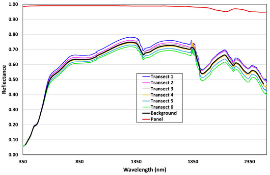
Figure 1.
Average signatures for six transects of the Pinnacles area, the panel and background reflectance.
The panel radiances taken in 11 groups between transects were tested for quality by plotting measured panel radiance against the cosine of solar zenith angle θs. Strictly, the total transmittance Ts in Equation (10) is also a function of θs, but it is a secondary effect. Good radiance data should have a high (near linear) relationship with cosine θs away from sunrise and noon The best data are in the later half of the set of measurements shown in Figure 2. The piecewise straight lines were used to define the panel value interpolations within transects used to obtain the reflectance values in Figure 1. The data were interpolated by time. Panel readings clearly off the line were rejected for future use.
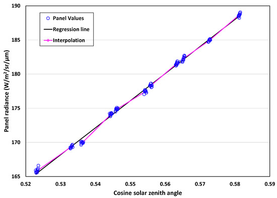
Figure 2.
The relationship between the individual panel radiance measurements averaged over all wavelengths and the cosine of solar zenith angle (θs).
As emphasized in [35], the leveling of the panel is essential to obtain useful data for radiometry and for accurate irradiance data. If a panel is not level, the irradiance is not proportional to the cosine of the solar zenith angle but rather to the cosine of the incident angle between the Sun and the sloping panel. The changes with time then depend on the angle between the azimuths of the panel slope and the solar azimuth, and if the slope is significant, the estimated irradiance will be biased. It is also important for any panels used to be close to Lambertian with few or no specular effects. The Labsphere panel quality is indicated by its high reflectance at all wavelengths (including the UVA), which is also plotted in Figure 1 for reference.
Three of the eleven groups were selected from the later part of the transect measurements. The three times (called t1, t2 and t3 in the following) were 10.317, 10.550 and 10.852 h local time of day (to be near satellite overpasses) with solar zenith angles of 57.8, 56.2 and 54.5 degrees. Each group of measurements consists of 10 replicates taken during less than 1 min. The three times (t1, t2 and t3) are the averages over times for the replicates with a group. Variation in measured irradiance over the 10 samples was estimated to be about 0.2% for 1 nm data, which would be less than 0.1% with 10 nm data. These variations show the atmosphere was very stable and do not provide a source of error in the data. The averaged total irradiance measurements at ASD-FR resolution for the three mean times are plotted in Figure 3. The ASD-FR data are also integrated to the 10 nm Band Set to illustrate the effect of the integration.
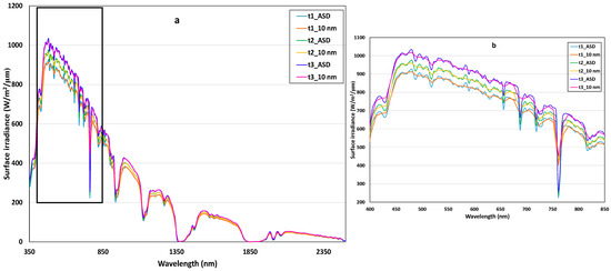
Figure 3.
Surface irradiance measurements for three different times (t1, t2, t3), where “ASD” means base ASD data at 1 nm sampling steps and “10 nm” means the ASD integrated to AVIRIS band-pass functions at close to 10 nm sampling steps. (a) for the wavelength 350–2500 nm; (b) for the wavelength 400–850 nm.
The “closer look” at Figure 3b shows that the 10 nm integrated data remove the high-frequency features noticeable in the base ASD-FR spectrum of the VNIR section (Figure 3b). However, in the SWIR, the ASD-FR and 10 nm resolution band data are effectively identical. Figure 3 also suggests that the ASD-FR resolution is possibly about 5 nm in the VNIR and about 10 nm in the SWIR and the UVA. There were some ancillary data collected during the measurements. A MICROTOPS II [36] was used to collect ozone data based on narrow bands in the region 300–350 nm. The output over a time period that included the three times t1, t2 and t3 estimated column ozone to be 0.2554 atm-cm with a variation of 8.5%. As field-measured water vapor and aerosol measurements were not available, some other information sources were accessed. The European Centre for Medium-Range Weather Forecasts (ECMWF) [37] data are provided globally at steps of 0.125 degrees and every 6 h, and [38] evaluated these data as the best reanalysis product in the Australian region. Interpolating for the Pinnacles site and date/time provided an estimate for ozone of 0.2853 atm-cm and an estimate for column water vapor of 0.6614 g cm−2. The ozone is similar, and the atmosphere was clearly very dry.
Aerosol levels in Australia are generally low. Mitchell et al. [39] divided the Australian climatology into tropical, arid and temperate zones. In the arid and temperate zones, the AOD550 is rarely above 0.1. The Pinnacles site is probably borderline to arid and temperate; in May, there would not have been any influence from seasonal fires, and no dust storms had occurred in this area in previous months. Qin et al. [40] used AATSR (the Advanced Along-Track Scanning Radiometer) data to develop a climatology of aerosol AOD for Australia that has been used in the GA time series [41]. The climatology data from the GA system provided an average AOD value of 0.0574 for an area covered by Landsat 8 images (path 113, row 81) containing the Pinnacles for May 20. Since the Pinnacles site is close to the coast, the AOD should be larger than the inland part of the averaging area. Therefore, it is reasonable to assume that the average AOD in May for Pinnacles is likely higher than this but less than 0.1.
4. Results
4.1. Model Evaluation Results from Landsat 8 and 9 Broadband Solar Spectrum Observations
In [3] and Section 2.1, it was proposed that the broadband E01 estimates from Landsat 8 OLI calibrations could be assumed close to the “true” values. In this case, the statistics rt (Equation (3)) and δrt (Equation (6)) can be used to compare solar spectra using their ratio to and relative difference from the “true” solar spectrum. These statistics can be directly computed from Table 2a,b. Changes from [3] are that the panchromatic band has been included in the analysis and the observed OLI solar spectrum has been calculated directly from the calibrations in the metadata file. These made only insignificant differences compared with the results in [3]. The OLI band 9 (1373.50 nm cirrus cloud band) estimate is also included in Table 2a. However, it has not been used in comparisons for reasons discussed earlier. For each band and each model, Table 3a lists the δrt value of Equation (6). The last three rows of Table 3a summarize the data. The mean indicates bias, the standard deviation is as normally defined and RMS is the root mean square over all bands of the δrt which are relative errors. The measure of performance is the RMS of the δrt over all bands. This is sensitive to large fractional errors occurring in some bands. For Landsat data with a few bands, a single outlier can indicate a major problem. The maximum absolute value of δrt for a single model is also significant information.
In [3], the Model 2 RMS (1.34%) was apparently “best” among the standard selections but was (and is) biased in the mean by about −1%. A “correction” was used to remove the apparent bias and created Model 5. The resulting Model 5 was better in the final figures (RMS < 1%) but has not been promoted due to possible overfitting from its “regression” correction. For individual bands, an absolute error of more than 3% (0.03) has been regarded as “poor” because differences of this relative magnitude often noticeably affected the image surface reflectance results. On this criterion, Models 1, 4 and 7 have a high positive bias in the coastal blue band; Model 4 has a negative bias in the SWIR, whereas Model 3 has high a negative bias in the NIR band.
Based on RMS, the ranking for the models included in [3] (Models 1–5) is unchanged from [3]. The order is Model 5 (0.94%) < Model 2 (1.34%) < Model 3 (2.20%) < Model 1 (2.52%) < Model 4 (3.37%). The three new models fall between Model 2 and Model 3 with Model 2 (1.34%) < Model 7 (1.39%) < Models 6 and 8 (1.47%) < Model 3 (2.20%). Li et al. [3] found that using radiance calibration with Models 1, 3 and 4 led to noticeable and often unacceptable differences in surface reflectance, especially in band 1, after atmospheric correction. On the other hand, Models 5 and 2 produced surface reflectance values close to those from the Landsat 8 TOA reflectance product.
Table 3b shows the same analysis as Table 3a but for Landsat 9 OLI2 data using the initial solar spectrum (as described in Section 3.1). The OLI2 band-pass models are not significantly different (about 0.2%) from OLI and have a negligible effect on the results between the instruments. The initial independent OLI2 solar spectrum observation (Table 2b) is about 1.5% different from that of OLI if Band 9 is not included. The general list of single-band differences above 3% mirror those from Table 3a with Models 1 and 4 having high bias in band 1, Model 4 again being high in the SWIR and Model 3 and Model 8 being high in the NIR. However, Model 7 is better in Band 1, and Models 3, 4 and 8 are above 3% in Band 3.
Table 3.
(a) δrt results from different solar spectrum models, where Mean, STD and RMS are the average, standard deviation and root mean square of the differences between the observed OLI solar spectrum and the selected solar spectrum model for 8 bands, respectively, where cwl is band central wavelength. (b) δrt results from different solar spectrum models, where Mean, STD and RMS are the average, standard deviation and root mean square of the differences between the observed OLI2 solar spectrum and the selected solar spectrum model for 8 bands, respectively, where cwl is band central wavelength. (c) δrt results from different solar spectrum models and the average solar spectrum of OLI and OLI2 observations, where “RMS” is the RMS of 8 bands for δrt and Max % is the maximum absolute δrt for an individual band.
| (a) | |||||||||
| Model | 1 | 2 | 3 | 4 | 5 | 6 | 7 | 8 | |
| Band | cwl (nm) | ||||||||
| 1 | 442.98 | 0.05849 | −0.00576 | 0.02621 | 0.04045 | 0.00631 | 0.01627 | 0.03115 | 0.02095 |
| 2 | 482.59 | −0.00447 | −0.01812 | −0.00638 | 0.00750 | −0.00619 | 0.00454 | 0.00125 | 0.00190 |
| 3 | 561.33 | −0.01052 | −0.01356 | 0.00808 | 0.02220 | −0.00160 | 0.00427 | −0.00326 | 0.00988 |
| 4 | 654.61 | 0.00380 | −0.00454 | −0.00125 | 0.01280 | 0.00760 | −0.00074 | 0.00284 | −0.00448 |
| 5 | 864.57 | 0.00915 | 0.00065 | −0.03946 | 0.00910 | 0.01281 | −0.01271 | 0.01236 | −0.02456 |
| 6 | 1609.10 | −0.02077 | −0.01451 | −0.01475 | −0.03525 | −0.00253 | −0.01512 | 0.00044 | −0.00544 |
| 7 | 2201.20 | −0.01816 | −0.02399 | −0.02411 | −0.05809 | −0.01214 | −0.02460 | −0.01131 | 0.00561 |
| 8 | 591.67 | 0.00523 | 0.00081 | 0.01604 | 0.03030 | 0.01297 | 0.01499 | 0.01037 | 0.01744 |
| Mean | 0.00284 | −0.00988 | −0.00445 | 0.00363 | 0.00215 | −0.00164 | 0.00548 | 0.00266 | |
| STD | 0.02499 | 0.00904 | 0.02154 | 0.03351 | 0.00916 | 0.01465 | 0.01275 | 0.01450 | |
| RMS | 0.02516 | 0.01339 | 0.02200 | 0.03371 | 0.00941 | 0.01474 | 0.01388 | 0.01474 | |
| (b) | |||||||||
| Model | 1 | 2 | 3 | 4 | 5 | 6 | 7 | 8 | |
| Band | cwl (nm) | ||||||||
| 1 | 442.76 | 0.05274 | −0.01172 | 0.02056 | 0.03476 | 0.00031 | 0.01007 | 0.02537 | 0.01515 |
| 2 | 482.30 | 0.01074 | −0.00311 | 0.00866 | 0.02279 | 0.00900 | 0.01984 | 0.01660 | 0.01721 |
| 3 | 560.92 | 0.01190 | 0.00890 | 0.03118 | 0.04561 | 0.02112 | 0.02718 | 0.01948 | 0.03302 |
| 4 | 654.30 | 0.01182 | 0.00355 | 0.00681 | 0.02090 | 0.01572 | 0.00745 | 0.01092 | 0.00361 |
| 5 | 864.61 | −0.00310 | −0.01152 | −0.05090 | −0.00318 | 0.00047 | −0.02482 | 0.00004 | −0.03656 |
| 6 | 1608.40 | −0.01298 | −0.00680 | −0.00709 | −0.02783 | 0.00526 | −0.00741 | 0.00828 | 0.00220 |
| 7 | 2201.10 | 0.00317 | −0.00278 | −0.00290 | −0.03775 | 0.00933 | −0.00340 | 0.01021 | 0.02749 |
| 8 | 593.95 | 0.00858 | 0.00402 | 0.01889 | 0.03318 | 0.01626 | 0.01778 | 0.01347 | 0.01988 |
| Mean | 0.010360 | −0.002433 | 0.003150 | 0.011058 | 0.009684 | 0.005833 | 0.013049 | 0.010253 | |
| STD | 0.019206 | 0.007506 | 0.025193 | 0.030651 | 0.007591 | 0.016968 | 0.007658 | 0.021650 | |
| RMS | 0.021822 | 0.007890 | 0.025389 | 0.032585 | 0.012305 | 0.017943 | 0.015130 | 0.023955 | |
| (c) | |||||||||
| Model | RMS | % | Max% | ||||||
| Model 5 | 0.00820 | 0.82 | 1.2 | ||||||
| Model 2 | 0.00832 | 0.83 | 1.3 | ||||||
| Model 7 | 0.01257 | 1.26 | 2.9 | ||||||
| Model 6 | 0.01473 | 1.47 | 1.9 | ||||||
| Model 8 | 0.01850 | 1.85 | 3.0 | ||||||
| Model 1 | 0.02242 | 2.24 | 5.6 | ||||||
| Model 3 | 0.02264 | 2.26 | 4.5 | ||||||
| Model 4 | 0.03236 | 3.24 | 4.8 | ||||||
In Table 3b, the results for Models 1–5 are generally similar to Landsat 8 data (Table 3a) with some exceptions. The order of the model performance for the common Models 1–5 is Model 2 (0.79%) < Model 5 (1.23%) < Model 1 (2.18%) < Model 3 (2.54%) < Model 4 (3.26%). Now Model 2 has become the best fitting. Model 5, derived by removing a bias, is next. Model 2 now has no significant mean bias. The new Models 6 and 7 are between Model 5 and Model 1, and Model 8 follows Model 1, with Model 5 (1.23%) < Model 7 (1.51%) < Model 6 (1.80%) < Model 1 (2.18%) < Model 8 (2.40%). Model 7 has the largest mean bias when compared with Landsat 9 data, and Model 8 changes the most between the two cases. In both the OLI (Table 3a) and OLI2 (Table 3b), the selected models, therefore, fall basically into three groups: firstly, Models 2 and 5 with an RMS at about 1%, then Models 6 and 7 at about 1.3–1.9% and finally Models 1, 3 and 4 at between 2 and 3% in each case. Model 8, however, is more variable between the cases.
The hypothetical “true” solar spectrum should not change with the sensor apart from (possibly) changes in band passes. As the band passes of OLI and OLI2 are essentially the same, the differences must be due to the calibration difference. However, which is closest to the “true” solar spectrum is not clear. If the individual band differences are examined, Bands 3 and 7 have more than a 2% difference between OLI and OLI2. Band 3 has played a significant part in the differences in percentages found above for OLI2 (especially for Model 8), and the differences may merit re-examination of the Landsat 9 calibrations in the future. Further relevant discussion can be found in [27].
A single conclusion can usefully be made from the two datasets. In both Landsat 8 OLI and Landsat 9 OLI2, the estimated solar spectra can be regarded as the “true” solar spectrum plus calibration errors. It is reasonable to assume that these errors are independent of the specific solar spectrum model selected as well as the “true” solar spectrum and are independent between OLIs. The average of the two should therefore be a better estimate of the “true” solar spectrum than either of the separate estimates and to balance the independent errors. A common conclusion has therefore been made using the average estimated solar spectrum. The complete Table 3a,b is not repeated for the average solar spectrum. Instead, Table 3c summarizes the rank order of models with RMS (%) for the average OLI and OLI2 estimated solar spectrum. Also included is the maximum absolute % δrt (Max %) among the individual bands for the model.
To summarize for the models that fit “well”, Models 2 and 5 persist in having the smallest RMS values and being close to 1% in all bands. The new Models 6, 7 and 8 at 1–2% will also produce values based on radiance that are similar to those based on top-of-atmosphere reflectance and be close to the “true” solar spectrum. However, Model 7 has a larger error at Band 1 than Model 6, and Model 8 has higher errors in Bands 3 and 5.
The findings from [3] suggested that Model 5 should be considered as the best candidate for the wavelengths involved in the Landsat sensors. However, based on the results of using the Landsat 9 (OLI2) independent observation and the combined average of OLI and OLI2, it is likely that Model 5 was overfitting and that Model 2 can be used instead for both sensors. In the Landsat 9 data, as well as in the average of OLI and OLI2, Model 2 fits at less than 1%, which is quite close. The simultaneous provision of solar diffuser-based reflectance and well-calibrated radiance products for the Landsat 8 OLI and Landsat 9 OLI2 has allowed consideration of the proposition that a small RMS indicates a model being close to the “best” solar spectrum. As discussed in [3], issues of calibration, which create the differences between the two solar spectrum observations used here, can potentially affect the selection of the “best” model. However, the differences observed do not change the findings that Model 2, Model 6 (which uses Model 2 SWIR values here) and Model 7 are the “best” under this criterion among the independent observations. Nor do they change the conclusion that Model 1, Model 3 and Model 4 have significant differences from the “best” solar spectrum. Model 8 is seen here to belong more with Models 2, 6 and 7 than with Models 1, 3 and 4.
4.2. Analysis of the Solar Spectra at 10 nm Resolution
Using the 10 nm Band Set aims to ensure the comparisons are at a consistent resolution scale. The solar spectrum models were integrated to this set of 221 bands to provide a realistic band set that is likely similar to the bands on current and future hyperspectral sensors. Plotting the results for all cases, as well as those observed for the OLI/OLI2 (Figure 4), it was found that differences between cases in the Landsat bands seen in the previous analysis are not independent or confined to the Landsat 8 or Landsat 9 bands but are due to much more systematic and persistent effects over wider spectral areas.
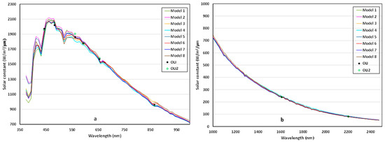
Figure 4.
Eight solar spectrum models integrated to the 10 nm Band Set resolution with OLI and OLI2 observations at central wavelength, where (a) shows the UVA and VNIR region 350–1000 nm and (b) plots the SWIR region 1000–2500 nm.
Viewed at 10 nm resolution, which could be regarded as a “continuum” scale by most scientists working with solar spectra, the differences previously found between choices of solar spectrum models are clear. The plotted Landsat observations need to be considered carefully (e.g., Band 8) as they are based on a broader bandwidth than 10 nm. Except for Model 4 and Model 8, the solar spectra seem to agree with each other in the SWIR at the plotting scale. This may be because they often use one of a small number of SWIR default models based on past measurements. The most obvious differences occur in the UVA, VNIR and NIR areas. However, many of the differences are outside of the Landsat band set. In the comparison between OLI and OLI2, the most striking difference is in Band 3 where the value plots away from the model selections.
In the development of Model 1 [25], Models 3 and 4 (each uses Thuillier et al., 2003 [9] in part or whole), Model 6 (Chance and Kurucz, 2010 [5]), Model 7 (TSIS−1, Coddington et al., 2021 [8]) and Model 8 (SOLAR-ISS, Meftah et al., 2020 [7]), the increasing number of space-borne instruments has been used to specifically help improve the UV solar spectrum models. The main differences in the UVA are between three sets of models. Models 2 and 5 are high, Model 1 is low and Models 3, 4, 6, 7 and 8 forming a cluster in between. Given the effort that has gone into these five models in the UVA, Model 3, Model 4, Model 6, Model 7 and Model 8 are the expected main candidates for best in the extended UVA/VNIR/SWIR range.
Of the five, Model 3 was a good model in the Landsat 8-based study in [3] but had some “splicing” error or another problem in the near-infrared (near 850 nm) which is still present. However, in the UVA, it is one of the “cluster” of UVA models above. Model 4 is biased low compared to the others over the 500–700 nm section of this range. This is opposite to a different bias in the SWIR (Figure 4). Nevertheless, the five selected models form a consistent set with a generally agreed value in the UVA. In relation to the Landsat 8 band 1, the value seemed high in OLI, and based on the work reported in [3], the OLI2 estimate would give better results. Bands 2 and 3 are higher for OLI2 than OLI and much higher for OLI2 in Band 3, suggesting this band, at least, may have a calibration issue. Unfortunately, apart from the few Landsat points which generally have coarser resolutions than 10 nm, there is no candidate “true” solar spectrum at 10 nm resolution with which to test the consequences of using Models 1–8. If there were, the δrt values could be calculated and an analysis similar to the previous Landsat-based study could be used.
4.3. Model Evaluation Results Based on Inversion of Surface Irradiance Observations
The report [19] used the inversion of data generated by MODTRAN data as a partial validation of the Irr_Inv software. One example used different solar spectrum models for the MODTRAN outputs and the Irr_Inv inversion models. The retrieved atmospheric parameters turned out to be physically unlikely and had a poor fit. When selected solar spectra were the same, the inversions worked well. It seemed that fitting atmospheric parameters could, in some cases, distinguish between the uses of different solar spectra. This observation led to using inversion to evaluate selections of the solar spectrum model as explained in Section 2.2.
The available data are panel-based estimates of total irradiance at various times. As discussed in Section 3.2 and the report in [19], inverting atmospheric parameters using only total irradiance can be achieved successfully with care in the provision of input data and parameter selection. To improve the stability of the inversions, the atmospheric parameters for the Pinnacles data were restricted to vary in a physically reasonable way by fixing the Ångström slope to 1.45. This is a likely value in the dry desert atmosphere. The atmosphere had low aerosol optical depth (believed to be <0.1) and was dry (W~0.6 g cm−2), as indicated by ancillary ECMWF data. The conditions were stable with very low cloud amounts, and the background reflectance was very bright (~0.7–0.8). Three groups of replicated panel estimates (t1, t2, t3) were selected from the panel readings.
The ASD-FR data and the background reflectance were integrated to 221 values using the 10 nm Band Set for inversion. As discussed before, this was done to put them on a similar footing in terms of resolution and scale so that significant differences in choices of solar spectrum will affect current and planned Earth observation data. The inversion of the irradiance started with parameters that were regarded as “reasonable” for the day, the type of atmosphere and the site with as much use of ancillary data as could be accessed. The resulting fits to data by inversion are summarized in Table 4. The major rows of the left-hand column of Table 4 indicate the time periods of the data collection, with the last major row being averages of the respective results in the first three. For each of the eight models used in this study, Table 4 records the final RMS, the aerosol optical depth (AOD550), water vapor (W) and ozone (Uoz). Ångström slope (n) is fixed. Column 11 is the average over the models, and column 12 is the coefficient of variation (%) over models. The mean RMS increases a little with time. However, the relative increase is not as high as the irradiance also increases. Apart from RMS, variations in parameters between times are not large. Atmospheric parameters may be expected to vary a little with time even for a stable atmosphere.
Table 4.
Inversion results for averaged panel total irradiance data at three different times (t1, t2 and t3) using eight different solar spectrum models, where RMS is the irradiance error (W/m2/μm), AOD550 is AOD at 550 nm, W is total water vapor (g/cm2), Uoz is ozone (ATM-cm) and n is Ångström slope.
Among the models, estimates of the parameters AOD550 (CV 47%) and Uoz (CV 26%) vary significantly between different models, but W (CV 5%) does not. Significantly, AOD550 and Uoz are being varied in each case to help fit the changing “shape” brought about by the selection of a different solar spectrum. Obviously, the atmosphere does not change with the choice of the solar spectrum. This “compensation” can, with more complex atmospheres, mask differences due only to a change in the solar spectrum. However, in this case, the CV of the various RMS values is 19%, indicating a wide spread of errors between cases which is due only to the selection of the solar spectrum despite the compensations, because of the stable and simple atmosphere with high background reflectance (Table 4).
In Table 4, the most persistent result is that Model 6 achieves the minimum error over solar spectra in all cases of choice of solar spectrum. In the early evaluation using OLI and OLI2 data, Model 6 and Model 7 were also among the best selections but not differentiated (Table 3). There is also a general stable ranking of goodness of fit between the models and data collections with some interchanges that are most likely due to atmospheric parameters compensating as previously described. For t1, the order is Model 6 < Model 7 < Model 3 < Model8 < Model 4 < Model 1< Model 2 < Model 5. For t2, it is Model 6 < Model 3 < Model 7 < Model 8 < Model 1 < Model 4 < Model 2 < Model 5. And for t3, it is Model 6 < Model 3 < Model 8 < Model 7 < Model 1 < Model 4 < Model 2 < Model 5. The generally poorer results for Models 2, 5 and 1 are consistent with the more recent improvements in the UVA implemented in the other models. Most important to emphasize is that these rankings are only due to differences in solar spectrum models and are independent of calibration or other errors in the data because these errors stay the same in every run.
As an indication of the goodness of “fit” in terms of the irradiance values being inverted, Figure 5 shows the t3 results in the UVA and VNIR for the five best models (Model 6, Model 7, Model 8, Model 3 and Model 4). Due to the broad frequency nature of the atmospheric parameters, and no absorption, only AOD controls changes in the UVA. The major differences between selections of the solar spectrum seem to be variations in the VNIR between about 440 nm and 1000 nm.
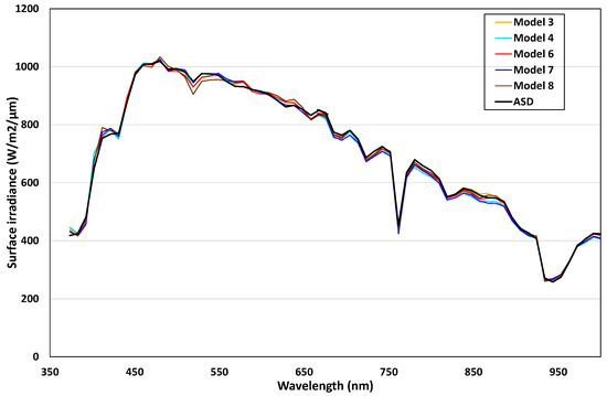
Figure 5.
Surface irradiance estimated from solar spectrum models and ASD-FR measurements for t3 for the 5 best spectrum models. All are integrated to the 10 nm Band Set bands.
The effects of atmospheric compensation can be seen clearly in these data by re-grouping them. Table 5 shows the results averaged separately for Models 2 and 5, Models 3, 4, 6, 7 and 8 and Model 1. The data are averaged over the three times to obtain a single value. For the first three columns, taking the five best models as “central”, Models 2 and 5 have compensated by increasing AOD to 0.172 (which, based on the information in Section 3.2, is too high for the location and day) and reducing ozone to 0.182—which is very low compared with the ancillary ozone data. In the opposite way, Model 1 reduces the AOD to a very low value and increases ozone to a very high value. These changes occur when forcing the “shape” in the UVA to the data when the solar spectrum changes.
Table 5.
Average inversion results for three different model groups, where RMS is irradiance error (W/m2/μm), AOD500 is AOD, W is total water vapor (g/cm2) and Uoz is ozone (ATM-cm).
While inversions based on least squares have a statistical interpretation, the differences between the selections of the solar spectrum are not statistical but systematic differences. The difference between the “true” solar spectrum and the selected solar spectrum is a systematic perturbation of the model. This perturbation allows some compensation by parameter variations from “true” as illustrated in Table 5. These changes represent errors in the parameter estimates from the attainable estimates.
The “best” solar spectrum can be proposed as the one that fits the data most closely using Irr_Inv (the “RMS” row in Table 4). However, a better total “result” in this situation should include both lower RMS and more acceptable results (less compensation or error) for the estimated aerosol, ozone and water vapor from an estimate for the “attainable” model. The “attainable” parameters are those obtained using the “true” solar spectrum. The evidence of significant compensation in Models 1, 2 and 5 in Table 5 is clear, and using this criterion, Model 6, Model 7, Model 8, Model 3 and Model 4 have been selected as the remaining candidates. The average values for the parameters for these selections are similar to the estimated MICROTOPS ozone over the time period (0.2554 atm-cm) and the regional ECMWF estimate for water vapor (0.6614 g cm−2). The AOD was expected to be larger than the climatological value 0.0574 as the Pinnacles site was nearer to the coast than the majority of the area where it was measured but less than 0.1. The average of 0.0831 is therefore also reasonable. The compensations by Models 1, 2 and 5 can also be seen as large errors in estimates of atmospheric parameters if these solar spectrum models are used for the estimation.
Applying the criterion of goodness of fit to the remaining selections using Table 4, Models 6, 3, 7 and 8 with average errors of 6.437, 6.883, 7.289 and 7.433 are separated from Model 4 with 8.159. To reach a final set, we have combined the results from the Landsat-based study (Study 1, Section 4.1) and the field irradiance study (Study 2, Section 4.3). Model 3 seems to have been adjusted from Model 4 with improvements, but one section was poorly spliced between the VNIR and the SWIR. This led to its poor performance when evaluated using Landsat OLI and OLI2 solar spectrum observations. The different measures of performance used in the two studies account for the different positions. The RMS of the relative errors () is less tolerant of local large errors. The conclusion based on combining the two studies is that Models 6, 7 and 8 are the best-performing models, with Model 6 being most persistently best in Study 2. Models 2 and 5 were rejected in the second study due to poor representation of the solar spectrum in the UV, and Model 3 was rejected because of the errors found in Study 1. Otherwise, the two studies are consistent.
4.4. Potential Change in Estimated Surface Reflectance with Change in Solar Spectrum
Li et al. [3] showed that the surface signature after atmospheric correction could have significant errors if incorrect solar spectrum models are used. In Section 2.1, Equation (7) was developed to model the variations found in estimates for surface reflectance in Landsat 8 images due only to different selections of the solar spectrum. To construct an application of Equation (7) for this paper, if MODTRAN is used to define the atmospheric terms, Model 6 is assumed to be the “true” solar spectrum and a signature is provided to represent the surface reflectance on the ground, then atmospheric correction of the simulated TOA radiance will obtain the signature provided if Model 6 is used. The possible variation in the estimated surface reflectance after atmospheric correction due to using another solar spectrum can then be simply computed from Equation (7). MODTRAN with settings the same as or similar to those used for Pinnacles can be used to provide the terms for Equation (7).
Li et al. [3] used an average of different land cover types to demonstrate variation in retrieved surface reflectance when different solar spectrum models are used. It is known from that work that darker signatures (such as coastal waters) will be most affected in the blue to UVA part of the spectrum and that very bright areas (such as clouds) maximally amplify differences at all wavelengths. Therefore, the selected dark and bright targets are used to demonstrate how the surface reflectance estimated by atmospheric correction can be affected by using different solar spectrum models. These extremes are sufficient to illustrate the result for the present paper. The darker example is coastal water in the north of Australia, and the second is simply the bright target signature of the Pinnacles area where ASD-FR data were collected. Both datasets are based on field measurements. An atmospheric state was assumed to run MODTRAN to compute . The atmosphere was given an AOD of 0.15 (higher than that at Pinnacles) and values for W of 0.484 and Uoz of 0.274 (similar to the Pinnacles atmosphere). With these settings, the ratio of surface reflectance values due to the choices of the solar spectrum can be computed from the selections based on Equation (7) and MODTRAN output . The magnitudes of AOD, W and Uoz will not impact the overall result patterns, but the magnitude of variation will increase for the darker target as AOD increases since the diffuse radiation will increase.
For the coastal water, the variation over all choices of solar spectrum used is shown in Figure 6. The estimated changes assume perfect calibrations. Overall, the variations previously noticed in Landsat 8 images in the coastal blue band [3] are repeated with increased effect in the UVA. Although it is not easy to see among the eight signatures in Figure 6, the differences obtained using Model 7 or Model 8 are similar to the assumed model signature for Model 6 with only a few small differences. Using the background signature from the Pinnacles, which is as high as 0.75–0.80 reflectance at some of the wavelengths measured, the above variations in the UVA/blue (where the background reflectance is small) are now relatively small. However, there are still some obvious variations in other wavelength regions that may require attention. These differences are now almost all due only to the ratio of the two solar spectra. Figure 7 plots them for both (a) UVA-VNIR and (b) SWIR areas.
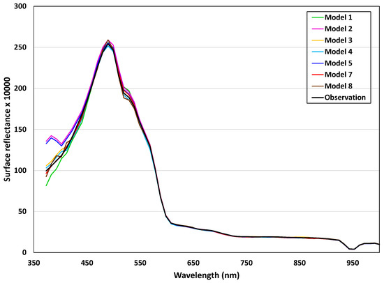
Figure 6.
The variation in water signatures using different solar spectrum models against Model 6.
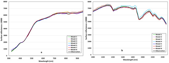
Figure 7.
The variation in desert signature using different solar spectrum models against Model 6, (a) for UV and VNIR (b) for SWIR.
The difference between using Model 6 and using Model 7 in both cases is mostly small except in the SWIR in Figure 7 where they separate slightly. To provide some ideas of magnitudes, the RMS difference between using Model 6 and Model 7 cases is 1% of the RMS of their average. The best RMS fits to the ASD-FR data at the 10 nm resolution were generally 1.5%. Because the background reflectance values used are high, differences in Figure 7a,b are magnified. Two obvious discrepancies are one in the near-infrared near 850 nm (Landsat 8 and 9 NIR band) and a high-biased case in the SWIR. The anomaly near the NIR band is in Model 3. It seems to have occurred during model construction. The high visible bias in the SWIR is due to Model 4. Model 8 also shows some differences from the others in the SWIR bands.
It has been concluded that Models 6, 7 and 8 are the best available based on the two studies, but there are remaining differences between the three. This final study of the stability of surface reflectance estimates shows that if Model 6 is taken as the “true” solar spectrum, then using either Model 7 or 8 will not make significant difference to estimated surface reflectance if calibrations are good and signal–noise ratio (SNR) is high. However, it seems the ideal would be if the remaining differences between these three models could be resolved to provide a common “best” model, at least at this scale of spectral resolution.
5. Discussion
5.1. Scale of Comparison
Using the 10 nm scale and hyperspectral data shows (Figure 4) what is creating the differences between the standard solar spectrum model selections used in the past. They are not random variations at a few band centers but rather systematic differences. In [3], it was shown that differences in the relative differences found in standard selections of the solar spectrum of perhaps 3% could create significant and noticeable variations in estimated surface reflectance from radiance products if the reflectance values are estimated using top-of-atmosphere radiance. One may argue that all sensors should be combined with accurate onboard panels or solar diffusers in the future. This can overcome the problems described as long as only surface reflectance products are needed and the reference solar diffuser is accurately characterized and calibrated. However, there are still many existing and planned sensors that do not or cannot (for various reasons) have accurate solar diffusers for reference. The differences observed seem likely to have come about through the combining and splicing of data from many solar radiation instruments at different resolutions from different platforms and at different times. Therefore, if these decisions are reviewed at 10 nm resolution and modified, there may be useful improvements made of value to many current and future missions.
5.2. Ancillary Information
The use of optimization to estimate atmospheric parameters as well as varying the selection of the solar spectrum to “rank” the performance of the solar spectra can give useful results. Sufficient ancillary data were obtained for this study to provide starting models and validation from standard sources such as the ECMWF [37]. However, in the future, especially if more sensitive instruments are used, it would be useful if additional accurately measured and independent ancillary values for the atmospheric parameters could also be available to support the conclusions. It would certainly also help to use the ECMWF profiles in MODTRAN and Irr_Inv with adjustments based on local meteorological data from a weather station. The problem, however, is that it is not always clear how to provide accurate and independently characterized observations. CIMEL and MICROTOPS sun photometer instruments have both been deployed at the site on other occasions. However, neither instrument is hyperspectral; their processing also assumes a solar spectrum, and the results are likely to have variance issues when aerosol levels are as low as in the present case. Standard processing of CIMEL data at AErosol RObotic NETwork (AERONET) [42,43] has often had difficulty with Australian low aerosol conditions. At one time, Australian data were processed routinely as described in [44,45]. The authors claimed that AOD could be measured from their network to 0.007 with 95% confidence. The methods were based on long-term monitoring and cross-calibration at a number of sites that included nephelometer and multiple sun photometer data. If similar precision for water vapor, ozone and possibly CO2 data could be obtained, they would certainly help in a future analysis of panel data to compare solar spectra.
6. Conclusions
Accurate solar spectrum models are essential for atmospheric correction and sensor calibrations for (lamp-)calibrated radiance satellites and, equally, for accurate estimates of atmospheric parameters from irradiance measurements. Five previously evaluated and three more recent solar spectrum models have been evaluated using the broadband Landsat 8 and 9 observations for the solar spectrum as well as independent surface irradiance observations. The results from the observed Landsat 8 and 9 solar spectra showed that Model 2 and Model 5 (both based on the work of Kurucz, 2005 [6]) with the more recent solar spectrum Model 6 (SA2010, Chance and Kurucz, 2010 [5]) and Model 7 (TSIS-1, Coddington et al., 2021 [8]) and Model 8 (SOLAR-ISS, Meftah, et al., 2020 [7]) obtained good results in the VNIR and SWIR bands. Although Model 4 (Thuillier et al., 2003 [9]) gave relatively good results in VNIR bands, it had poor performance in SWIR bands. The results (order of agreement) for the previously studied Models 1, 2, 3, 4 and 5 using the observed Landsat 8 and 9 solar spectra were essentially the same as those found in [3].
The Landsat 8 and 9 solar spectra are broadband and contained in the VNIR and SWIR spectral regions. The selected eight solar spectrum models were therefore further analyzed and examined in detail at higher spectral resolution (10 nm) and over an extended wavelength range from UVA to SWIR (370–2480 nm) using field solar irradiance measurements. The consequences of differences in the choice of solar spectrum model were evaluated by differences they create when using inversion of the parameters. The results showed that Models 6, 7 and 8 gave the best results, including in the UVA region. It is hard to distinguish the performance of Models 6, 7 and 8 apart from the observation that Model 6 persistently gives a lower RMS fit to field data. The eight solar models were also used to test how the surface reflectance estimate from a calibrated radiance sensor would change if different solar spectrum models were used. This is an application of Equation (7). Using dark (water) and bright (desert) signatures, the differences were simulated. If one of the best three models is assumed to be the “true” solar spectrum (in this case, Model 6), then using another will not significantly alter the estimated ground reflectance. On the other hand, the rest of the candidates gave differences (some large) in varying wavelength areas.
Although Model 4 had a similar UVA response to the best models in this study, its biases in SWIR region meant that it should be replaced by one of Models 6, 7 and 8. Models 2 and 5, which had the best performance for the Landsat 8 and 9 bands, had poor performance in the UVA region which removed them from consideration. CEOS recently replaced the Thuillier SOLSPEC Model 4 with the Coddington TSIS-1 Model 7 as the recommended solar spectrum model for Earth observation. This paper shows how this change represents a significant improvement in accuracy for applications, including the analysis of data from field instruments. However, the remaining differences found in this paper suggest it is still useful to review Models 6, 7 and 8 to possibly achieve a better overall result for current and future applications at 5–10 nm resolution.
Author Contributions
F.L. and D.L.B.J.: Conceptualization, Methodology, Software, Formal Analysis, Investigation, Writing—Original Draft Preparation, Writing—Review and Editing; B.L.M.: Formal Analysis, Resources, Writing—Review and Editing; I.C.L., C.O., G.B., T.M. and P.F.: Validation, Resources, Data Curation; M.T.: Validation, Project Administration; S.O.: Supervision, Writing—Review and Editing, Project Administration. All authors have read and agreed to the published version of the manuscript.
Funding
This research received no external funding.
Data Availability Statement
The dataset used in this research is available upon a valid request to any of the authors of this research article.
Acknowledgments
This paper is published with the permission of the CEO, Geoscience Australia, and of CSIRO (Australia). The MODTRAN® 6 radiative transfer software was used in calculations, and information has been taken from the User Manual (Berk et al. [20]). The Landsat 8 and calibration solar spectrum estimates were provided by the USGS and NASA. Fieldspec is a registered trademark of Malvern Pan Analytical. The authors thank Mark Broomhall and Zhi Huang of GA for reading an early draft and making valuable suggestions. Two anonymous reviewers made comments and suggestions that improved the paper. The Editors of MDPI have provided valuable input that has improved the style and clarity of the manuscript.
Conflicts of Interest
The authors declare no conflict of interest.
References
- Thome, K.J.; Biggar, S.F.; Slater, P.N. Effects of assumed solar spectral irradiance on intercomparisons of Earth-observing sensors. Proc. SPIE 2001, 4540, 260–269. [Google Scholar] [CrossRef]
- Fröhlich, C. Solar irradiance variability. In Solar Variability and Its Effects on Climate; Geophysical Monograph 141; AGU: Washington, DC, USA, 2004; pp. 97–110. [Google Scholar]
- Li, F.; Jupp, D.L.B.; Sagar, S.; Schroeder, T. The Impact of Choice of Solar Spectral Irradiance Model on Atmospheric Correction of Landsat 8 OLI Satellite Data. IEEE Trans. Geosci. Remote Sens. 2021, 59, 4094–4104, Erratum in IEEE Trans. Geosci. Remote Sens. 2021, 59, 5388–5388. [Google Scholar] [CrossRef]
- Markham, B.; Barsi, J.; Kvaran, G.; Ong, L.; Kaita, E.; Biggar, S.; Czapla-Myers, J.; Mishra, N.; Helder, D. Landsat-8 Operational Land Imager radiometric calibration and stability. Remote Sens. 2014, 6, 12275–12308. [Google Scholar] [CrossRef]
- Chance, K.; Kurucz, R.L. An improved high-resolution solar reference spectrum for Earth’s atmosphere measurements in the ultraviolet visible and near infrared. J. Quant. Spectrosc. Radiat. Transf. 2010, 111, 1289–1295. [Google Scholar] [CrossRef]
- Kurucz, R. High Resolution Irradiance Spectrum from 300 to 1000 nm. Available online: https://arxiv.org/pdf/astro-ph/0605029.pdf (accessed on 1 August 2019).
- Meftah, M.; Damé, L.; Bolsée, D.; Pereira, N.; Snow, M.; Weber, M.; Bramstedt, K.; Hilbig, T.; Cessateur, G.; Boudjella, M.-Y.; et al. A New Version of the SOLAR-ISS Spectrum Covering the 165–3000 nm Spectral Region. Sol. Phys. 2020, 295, 14. [Google Scholar] [CrossRef]
- Coddington, O.M.; Richard, E.C.; Harber, D.; Pilewskie, P.; Woods, T.N.; Chance, K.; Liu, X.; Sun, K. The TSIS-1 Hybrid Solar Reference Spectrum. Geophys. Res. Lett. 2021, 48, e2020GL091709. [Google Scholar] [CrossRef]
- Thuillier, G.; Herse, M.; Labs, D.; Foujols, T.; Peetermans, W.; Gillotay, D.; Simon, P.C.; Mandel, H. The solar spectral irradiance from 200 to 2400 nm as measured by SOLSPEC Spectrometer from the ATLAS and EURECA missions. Sol. Phys. 2003, 214, 1–22. [Google Scholar] [CrossRef]
- Green, R. (Ed.) HyspIRI Final Report, HyspIRI Mission Concept Team. NASA & JPL. 2018. Available online: https://hyspiri.jpl.nasa.gov/ (accessed on 1 February 2021).
- Loizzo, R.; Guarini, R.; Longo, F.; Scopa, T.; Formaro, R.; Facchinetti, C.; Varacalli, G.N. Prisma: The Italian Hyperspectral Mission. In Proceedings of the IGARSS 2018—2018 IEEE International Geoscience and Remote Sensing Symposium, Valencia, Spain, 22–27 July 2018; pp. 175–178. [Google Scholar] [CrossRef]
- ENMAP. Environmental Mapping and Analysis Program, DLR, Germany. Available online: https://www.enmap.org/ (accessed on 1 October 2022).
- Senese, S.; Thiel, M.; König, B.; Sornig, M.; Fischer, S.; Bergander, A.; Brunner, S.; Müller, S.; Schmidt, T.; Zajac, K. Full aperture diffuser assembly, fully redundant and high reliable optic mechanism for ENMAP mission. In Proceedings of the ‘ESMATS 2017’, Hatfield, UK, 20–22 September 2017; Available online: https://esmats.eu/esmatspapers/pastpapers/pdfs/2017/senese.pdf (accessed on 1 October 2022).
- EMIT. Earth Surface Mineral Dust Source Investigation. NASA EOS. Available online: https://eospso.gsfc.nasa.gov/missions/earth-surface-mineral-dust-source-investigation-evi-4 (accessed on 1 October 2022).
- Kopp, G.; Lawrence, G.; Rottman, G. The Total Irradiance Monitor (TIM): Science results. Sol. Phys. 2005, 230, 129–139. [Google Scholar] [CrossRef]
- Lean, J.L.; Coddington, O.; Marchenko, S.V.; Machol, J.; DeLand, M.T.; Kopp, G. Solar Irradiance Variability: Modeling the Measurements. Earth Space Sci. 2020, 7, e2019EA000645. [Google Scholar] [CrossRef]
- Rochford, P.A.; Acharya, P.K.; Adler-Golden, S.M.; Berk, A.; Bernstein, L.S.; Matthew, M.W.; Richtsmeier, S.C.; Gulick, S.; Slusser, J. Validation and Refinement of Hyperspectral/Multispectral Atmospheric Compensation using Shadowband Radiometers. IEEE Trans. Geosci. Remote Sens. 2005, 43, 2898–2907. [Google Scholar] [CrossRef]
- Byrne, G.; Walsh, A.; Thankappan, M.; Broomhall, M.; Hay, E. DEA Analysis Ready Data: Phase 1 Validation Project Report; Data Summary; Geoscience Australia: Canberra, Australia, 2022. [Google Scholar] [CrossRef]
- Jupp, D.L.B.; Li, F.; Byrne, G.; Ong, C.; Lau, I.; Malthus, T.; Thankappan, M.; Fearns, P. Using Irr_Inv, MODTRAN and Spectral Irradiance data to Estimate Atmospheric Parameters; CSIRO Report EP2022-3491; CSIRO: Canberra, Australia, 2022. [CrossRef]
- Berk, A.; van den Bosch, J.; Hawes, F.; Perkins, T.; Conforti, P.F.; Acharya, P.K.; Anderson, G.P.; Kennett, R.G. MODTRAN 6.0 User’s Manual. 2019. Available online: http://MODTRAN.spectral.com/ (accessed on 1 January 2020).
- Thompson, D.R.; Gao, B.C.; Green, R.O.; Roberts, D.A.; Dennison, P.E.; Lundeen, S.R. Atmospheric correction for global mapping spectroscopy: ATREM advances for the HyspIRI preparatory campaign. Remote Sens. Environ. 2015, 167, 64–77. [Google Scholar] [CrossRef]
- Pearlman, J.S.; Crawford, M.; Jupp, D.L.B.; Ungar, S. Foreword to the earth observing 1 special issue. IEEE Trans. Geosci. Remote Sens. 2003, 41, 1147–1148. [Google Scholar] [CrossRef]
- Green, R.O.; Mahowald, N.; Ung, C.; Thompson, D.R.; Bator, L.; Bennet, M.; Bernas, M.; Blackway, N.; Bradley, C.; Cha, J.; et al. The Earth Surface Mineral Dust Source Investigation: An Earth Science Imaging Spectroscopy Mission. In Proceedings of the 2020 IEEE Aerospace Conference, Big Sky, MT, USA, 7–14 March 2020; pp. 1–15. [Google Scholar]
- Ångström, A. The parameters of atmospheric turbidity. Tellus 1964, 16, 64–75. [Google Scholar] [CrossRef]
- Fontenla, J.M.; Harder, J.; Livingston, W.; Snow, M.; Woods, T. High-resolution solar spectral irradiance from extreme ultraviolet to far infrared. J. Geophys. Res. 2011, 116. [Google Scholar] [CrossRef]
- CEOS. Recommended Solar Irradiance Spectrum for Use in Earth Observation Applications. 2006. Available online: https://eocalibration.wordpress.com/2006/12/ (accessed on 1 August 2019).
- Gross, G.; Helder, D.; Begeman, C.; Leigh, L.; Kaewmanee, M.; Shah, R. Initial cross-calibration of Landsat 8 and Landsat 9 using the simultaneous underfly event. Remote Sens. 2022, 14, 2418. [Google Scholar] [CrossRef]
- Morfitt, R.; Barsi, J.; Levy, R.; Markham, B.; Micijevic, E.; Ong, L.; Scaramuzza, P.; Vanderwerff, K. Landsat-8 Operational Land Imager (OLI) Radiometric Performance On-Orbit. Remote Sens. 2015, 7, 2208–2237. [Google Scholar] [CrossRef]
- Markham, B.; Barsi, J.; (NASA Biospheric Sciences Laboratory, Greenbelt, MD, USA). Personal communication, 2022.
- Patrick, H.; Zarobila, C.; Germer, T. The NIST Robotic Optical Scatter Instrument (ROSI) and its Application to BRDF Measurements of Diffuse Reflectance Standards for Remote Sensing. Proc. SPIE 2013, 8866, 886615. [Google Scholar] [CrossRef]
- Ong, C.; Caccetta, M.; Lau, I.C.; Ong, L.; Middleton, E. Compositional characterisation of the pinnacles vicarious calibration site. In Proceedings of the IEEE International Geoscience and Remote Sensing Symposium (IGARSS), Fort Worth, TX, USA, 23–28 July 2017; pp. 3059–3062. [Google Scholar] [CrossRef]
- ASD. Fieldspec® 4 User Manual. ASD Document 600540 Rev. J. 2016. Available online: https://www.malvernpanalytical.com/en/products/product-range/asd-range/fieldspec-range (accessed on 1 May 2021).
- Malthus, T.; Ong, C.; Lau, I.; Fearns, P.; Byrne, G.; Thankappan, M.; Chisholm, L.; Suarez Barranco, L.; Clarke, K.; Scarth, P.; et al. A Community Approach to the Standardised Validation of Surface Reflectance Data—A Technical Handbook to Support the Collection of Field Reflectance Data; CSIRO Report EP183233; CSIRO Centre for Earth Observation: Brisbane, Australia, 2019. [CrossRef]
- Lau, I.C.; Thapar, N. Laboratory Spectroscopy Calibration Procedures, Version 2.0; CSIRO Report EP147766; CSIRO: Kensington, Australia, 2015. [CrossRef]
- Ruddick, K.G.; Voss, K.; Banks, A.C.; Boss, E.; Castagna, A.; Frouin, R.; Hieronymi, M.; Jamet, C.; Johnson, B.C.; Kuusk, J.; et al. A Review of Protocols for Fiducial Reference Measurements of Downwelling Irradiance for the Validation of Satellite Remote Sensing Data over Water. Remote Sens. 2019, 11, 1742. [Google Scholar] [CrossRef]
- Morys, M.; Mims, F.M.; Hagerup, S.; Anderson, S.E.; Baker, A.; Kia, J.; Walkup, T. Design, calibration, and performance of MICROTOPS II handheld ozone monitor and Sun photometer. J. Geophys. Res. Atmos. 2001, 106, 14573–14582. [Google Scholar] [CrossRef]
- Dee, D.P.; Uppala, S.M.; Simmons, A.J.; Berrisford, P.; Poli, P.; Kobayashi, S.; Andrae, U.; Balmaseda, M.A.; Balsamo, G.; Bauer, D.P.; et al. The ERA-Interim Reanalysis: Configuration and Performance of the Data Assimilation System. Q. J. R. Meteorol. Soc. 2011, 137, 553–597. [Google Scholar] [CrossRef]
- Li, F.; Jupp, D.L.B.; Thankappan, M.; Wang, L.W.; Sixsmith, J.; Lewis, A.; Held, A. Land surface brightness temperature retrieved from Landsat data. In Proceedings of the 21st International Congress on Modelling and Simulation, Gold Coast, Australia, 29 November–4 December 2015. [Google Scholar]
- Mitchell, R.M.; Forgan, B.W.; Campbell, S.K. The climatology of Australian aerosol. Atmos. Chem. Phys. 2017, 17, 5131–5154. [Google Scholar] [CrossRef]
- Qin, Y.; Mitchell, R.; Forgan, B.W. Characterizing the Aerosol and Surface Reflectance Over Australia Using AATSR. IEEE Trans. Geosci. Remote Sens. 2015, 53, 6163–6182. [Google Scholar] [CrossRef]
- Geoscience Australia 2022. Available online: https://cmi.ga.gov.au/data-products/dea/365/dea-surface-reflectance-landsat-8-oli-tirs (accessed on 17 February 2022).
- Holben, B.; Eck, T.; Slutsker, I.; Tanré, D.; Buis, J.; Setzer, A.; Vermote, E.; Reagan, J.; Kaufman, Y.; Nakajima, T.; et al. AERONET—A Federated Instrument Network and Data Archive for Aerosol Characterization. Remote Sens. Environ. 1998, 66, 1–16. [Google Scholar] [CrossRef]
- Holben, B.N.; Tanré, D.; Smirnov, A.; Eck, T.F.; Slutsker, I.; Abuhassan, N.; Newcomb, W.W.; Schafer, J.S.; Chatenet, B.; Lavenu, F.; et al. An emerging ground-based aerosol climatology: Aerosol optical depth from AERONET. J. Geophys. Res. Space Phys. 2001, 106, 12067–12097. [Google Scholar] [CrossRef]
- Mitchell, R.M.; Forgan, B.W. Aerosol measurements in the Australian Outback: Intercomparison of sun photometers. J. Atmos. Ocean. Technol. 2003, 20, 54–66. [Google Scholar] [CrossRef]
- Mitchell, R.M.; Campbell, S.K.; Qin, Y.; Gras, J. Performance characteristics of integrating nephelometers in the Australian Outback. J. Atmos. Ocean. Technol. 2009, 26, 984–995. [Google Scholar] [CrossRef]


Disclaimer/Publisher’s Note: The statements, opinions and data contained in all publications are solely those of the individual author(s) and contributor(s) and not of MDPI and/or the editor(s). MDPI and/or the editor(s) disclaim responsibility for any injury to people or property resulting from any ideas, methods, instructions or products referred to in the content. |
© 2023 by the authors. Licensee MDPI, Basel, Switzerland. This article is an open access article distributed under the terms and conditions of the Creative Commons Attribution (CC BY) license (https://creativecommons.org/licenses/by/4.0/).