Abstract
The bidirectional reflectance distribution function (BRDF) factor ƒ′ provides a bridge between the inherent and apparent optical properties (IOPs and AOPs) of inland waters. The previous BRDF studies focused on ocean waters, while few studies examine inland waters. It is meaningful to improve the theory of remote sensing of water surface and the accuracy of image derivation in inland waters. In this study, radiative transfer simulation was applied to calculate the ƒ′ values using appropriate IOPs based on in situ combined with realistic boundary conditions (N = 11,232). This study shows that ƒ′ factor varied over the range of 0.33–16.64 in Lake Nansihu, a finite depth water, higher than the range observed for the ocean (0.3–0.6). Our results demonstrate that the factor ƒ′ depends on not only solar zenith angle () but also the average number of collisions () and particulate backscattering ratio (). The ƒ′ factor shows a continuous geometric increase as the solar zenith angle increases at 400–650 nm but is relatively insensitive to solar angle in the 650–750 nm range in which ƒ′ increases as and decreases. To account for these findings, two empirical models for ƒ′ factor as a function of , and are proposed in various spectral wavelengths for Lake Nansihu waters. Our results are crucial for obtaining Hyperspectral normalized reflectance or normalized water-leaving radiance and improving the accuracy of satellite products.
1. Introduction
The ability to model the irradiance distribution in inland waters is a fundamental step in the development of advanced remote sensing techniques that can accurately determine the optically significant components. The irradiance reflectance just below the surface (, where and are the upward and downward irradiances just beneath the water surface) contains necessary information about the constituents of the water [1,2], as apparent optical properties (AOPs) are largely determined by inherent optical properties (IOPs). Assessing the relationship between and IOPs is valuable, as it enables estimation of IOPs from irradiance reflectance, which is more easily measured [2,3], for use in the theory of water color remote sensing. The most widely used remote sensing optical algorithm is expressed as [1,4,5].
where and are the total absorption and backscattering coefficients, respectively. is a distribution factor that depends on the solar zenith angle (), wavelength (), volume scattering functions (VSFs, ), surface roughness (via the wind speed, W), and aerosol optical thickness () [2,3,4,6,7,8,9]. The coefficient should be used if is not small with respect to , and the relationship between and is expressed as , where and are approximately 0.3–0.6 for all natural waters [10]. Variability in the or factor and its influence on remote sensing of ocean color have been the focus of several theoretical studies [2,3,6,7,11,12,13]. Kirk [2] proposed an approximation that is a function of the cosine of the in-water sun angle and obtained values in the range of 0.3–0.6; Morel et al. [6] established a lookup table for the factor, dependent on () and the chlorophyll concentration in open ocean waters. This method was adopted by the National Aeronautics and Space Administration and has become a standard method. However, it works well only with ocean waters and with a maximum chlorophyll concentration of 10 mg/m3, obviously not with inland waters. Previous studies of bidirectional reflectance factor were restricted to oceanic and coastal waters [6,7,8], but the variation of factor in inland Lakes remains unknown. The complex behavior of photons in inland waters resulting from the combined effects of the absorption and scattering coefficients, VSFs, and optically shallow bottoms, remains unclear. Further studies are needed for inland waters, which are impacted by human activities and have extremely complex apparent optical properties.
The current factor models are built using one or two VSFs since the VSFs measurement over broad angular ranges has been uncommon [14,15,16]. Particulate scattering is an important process determining both light penetrations through the water and light leaving the water. Further elucidation of the impact of the particulate backscattering ratio on or remains an important challenge. Therefore, investigation of the relationship between the particulate backscattering ratio (, where and are particulate scattering and backscattering, respectively) and or is very meaningful. As a result, the previous studies had a few focus on the effect of the VSFs on the bidirectional reflectance factor. He et al. [7] developed a bidirectional subsurface remote sensing reflectance model accounting for paticle backscattering shapes for an optically deep ocean, and it was requried to measure VSFs as a input, which was hard to apply the inland lakes because of the bottom reflectance and VSFs measurement. The particulate backscattering ratio, , supports the derivation of an approximate scattering phase function. As a result, has been used to generate a particulate phase function based on Mie theory and the Fournier–Forand phase function [17,18]. This ratio can be assumed to be spectrally constant [19,20]. Surface values range between 0.0004 and 0.06 [19,21,22,23,24,25,26,27,28], and particles in lakes are often divided into chlorophyll-bearing particles and mineral particles. According to the information available about the particulate composition and previous studies, 16 values of the chlorophyll-bearing particle ratio, , were selected from 0.005 to 0.018 at an interval of 0.001, as well as 0.0024 and 0.0183 [29]. For the mineral particle ratio, , 13 values from 0.01 to 0.06 at an interval of 0.005 as well as 0.013 and 0.0183 were used in this study.
2. Materials and Methods
2.1. Radiative Transfer Basic Theory
The RTE can predict underwater radiance distributions given the IOPs and boundary conditions of the water body. The HydroLight solves the integrodifferential RTE along with its boundary conditions based on the time-independent and one-dimensional (unpolarized, depth-dependent) light field in horizontally homogeneous water bodies using the invariant embedding method. Directions are specified via an x–y–z cartesian coordinate system using the nadir angle and azimuth angle with the x–y plane parallel to the water surface, with the +x and +z axis directions representing downwind and downward, respectively. The vector denotes a unit vector pointing in the desired direction, defined as follows.
where , , and are unit vectors in the x, y, and z directions, respectively. is the polar angle measured from the nadir direction , and the azimuth angle increases counterclockwise from , with values in the ranges and , respectively. The standard form of the RTE for radiance propagating in the water is [30].
where is the beam attenuation coefficient at geometric depth z and wavelength . The collection of all directions is designated the unit sphere , which comprises all values such that and . The volume scattering functions (VSFs) from the direction to the direction is denoted as . The quantity is the differential solid angle surrounding , and integration is conducted over the entire range of solid angles. Note that the solid angle measurement of the entire set of all directions is , as the area of a sphere is (solid angle ). The effective source term S is considered to include bioluminescence and inelastic scattering. In this paper, bioluminescence was not included, but we considered various inelastic scattering processes, such as chlorophyll and CDOM fluorescence, as well as Raman scattering by water; these processes are particularly important at longer wavelengths.
The RTE (Equation (3)) expressed in terms of the dimensionless optical depth as the relationship between and the beam attenuation coefficient c(z), as well as the geometric depth z () is
where is the volume scattering phase function (, where and are the VSFs and total scattering coefficient, respectively, with units of sr−1). is the single-scattering albedo, . The beam attenuation coefficient c can be expressed as , where is the absorption coefficient. Equation (4) shows all quantities as a function of . The total scattering coefficient b is given by [12].
The backscattering coefficient is defined as [21].
where is the scattering angle, and represents solid angles.
The downward and upwelling irradiances can be derived from the radiance through integration. The spectral downward plane irradiance beneath the water surface is expressed as [3,31].
and the spectral upward irradiance at null depth as [3]
where and are the upward and downward hemispheres of direction, respectively.
Additionally, defined by
2.2. Inherent Optical Properties Model
In radiative transfer simulations, IOPs (e.g., , , c, , and ) are necessary input quantities used as geometric functions in equations and models. We assumed that the study area (Lake Nansihu) is a homogeneous water body in which IOPs do not change with depth. The IOP parameters were computed on the basis of the following models. The spectral total absorption coefficient was calculated as follows [32]:
where , , , and are the absorption coefficients of pure water, CDOM, phytoplankton, and non-algal (mineral) particles, respectively. was obtained from Pope et al. (1997) [33]. The terms and can be expressed as multiply normalized chlorophyll-specific or mass-specific absorption [34,35] for each chlorophyll or mineral particle concentration ( or ). was calculated as [36].
Equation (9) can be expressed as
The spectral total scattering coefficient was calculated as follows [12]:
and the spectral particles scattering coefficient was determined as [37]:
where is the particle concentration, which is equal to plus and VSFs is [29]:
The volume scattering phase function can be written as [38]:
The spectral total backscattering coefficient was calculated as follows [21]:
where and are the backscattering coefficients of pure water and total suspended particles (phytoplankton and mineral particle ), respectively. and were obtained from Zhang et al. [39]. is half of the total molecular scattering coefficient, , and the backscattering ratio . The particle phase function with the values from 0.0004 to 0.06 [29] were applied to the RTE in this study. For the chlorophyll-bearing particle ratio, , 15 values were selected, including 0.005 to 0.018 at an interval of 0.001 as well as 0.0024 and 0.0183. For the mineral particle ratio, , 12 values from 0.01 to 0.06 at an interval of 0.005 as well as 0.0183 were used.
The average number of collisions, , is an intuitively efficient representation of diffuseness inside the radiant field, which is, in turn, directly related to the factor [12]. The experienced by photons before they escape from water can be expressed as: or , where is the single-scattering albedo, , and a and b are the absorption and scattering coefficients, respectively. Notably, we used rather than because is unbounded and more intuitive than [13], especially when multiple scattering is dominant in inland waters.
2.3. Input Parameters
The input parameters for Lake Nansihu simulations included chlorophyll-a and particulate concentrations, as well as depth and solar zenith angle based on in situ data (Table 1) collected in the region of the lake, namely, 34°33′29″–34°39′49″N and 117°11′12″–117°18′52″E. Particulate material (TSM) was collected on 25 mm Whatman GF/F glass fiber filters. Chlorophyll-a concentration (Chla) was collected in 47 mm GF/F glass fiber filters and measured [40]. Solar zenith was computed by the time in situ.

Table 1.
Data were collected at 27 sites during a Lake Nansihu cruise in 2015.
The radiative transfer simulations were conducted using the HydroLight 6.0 code with the following input parameters in addition to the parameters listed in Table 1:
- Wavelength, (100 values, from 400 nm to 750 nm at an interval of 5 nm)
- Bottom reflectance (macrophytes and clean seagrass, Figure 1a)
- Chlorophyll-bearing particle ratio, (16 values, from 0.005 to 0.018 at an interval of 0.001 as well as 0.0024 and the Petzold average of 0.0183)
- Mineral particle ratio, (13 values, from 0.01 to 0.06 at an interval of 0.005 as well as 0.013 and the Petzold average of 0.0183).
- CDOM (0.30 m−1 at 440 nm)
- Wind speed: 5 m/s
- Real index of refraction, n: 1.34
- Cloud coverage: 0%
- Airmass type: continental
- Relative humidity: 80.0%
- Aerosol optical thickness at 550 nm: 0.261
- Total ozone: 300.0 Dobson units

Figure 1.
(a) Bottom irradiance reflectance spectra obtained from HydroLight; (b) Phase functions of particles with backscatter fractions from 0.0024 to 0.06 and pure water with scattering angle.
Figure 1.
(a) Bottom irradiance reflectance spectra obtained from HydroLight; (b) Phase functions of particles with backscatter fractions from 0.0024 to 0.06 and pure water with scattering angle.

Two bottom types, the clean seagrass, and macrophyte, were used as provided with HydroLight 6.0 (Figure 1a). The average clean seagrass reflectance was based on measurements between 350 and 800 nm of 100% Thalassia measured by R. Zimmerman at Lee Stocking Island, Bahamas. Additionally, the Bottom reflectance spectrum for the average macrophyte is based on measurements between 400 and 750 nm taken near Lee Stocking Island, Bahamas, during the Coastal Benthic Optical Properties (CoBOP) experiment. Particle phase functions with Petzold average [29] and Fournier–Forand [18] values of from 0.0024 to 0.06 were used for the numerical simulations (Figure 1b). The scattering phase function for pure water was presented by Zhang et al. [39].
In addition, normalized sky radiances were computed using the Harrison and Coombes normalized sky radiance model [41]. Diffuse and direct sky irradiances were computed using the RADTRANX model [42]. Chlorophyll fluorescence quantum efficiency was set to 0.020, and the CDOM absorption coefficient used for the fluorescence calculation was obtained from the CDOM component of the IOP model. Raman scattering was included in this run, with a Raman scattering coefficient of 2.60 × 10⁻⁴ m−1 at the reference wavelength of 488 nm. The azimuthally isotropic Cox–Munk surface model was used for the surface simulation. The flow chart of factor calculation was shown in Figure 2. In this study, radiative transfer simulation was applied to calculate the ƒ′ values using the above IOPs models based on concentrations data of Chla, TSM, and CDOM combined with realistic boundary conditions, including sky radiance, sea state, bottom BRDF, and fluorescence. factor for 16 values, 13 values, and 2 bottom reflectance was calculated at 27 stations, and the total amount of factor was 11,232 (N = 11,232).
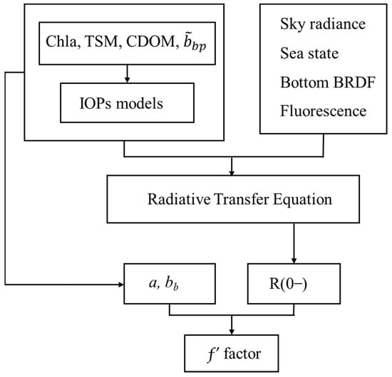
Figure 2.
The flow chart of factor calculation in Nansihu Lake.
3. Results and Discussion
The irradiance reflectance that is just below the surface, , was simulated with HydroLight. The value of factor equals the ratio between and . The relationship between and is shown in Figure 3. The black solid dot represents our simulated values obtained using the radiative transfer model described above. We compared several classical models with our results (Figure 3), which is larger than the value of 0.33 reported by Morel and Prieur (1977) [1]. The green and grey regions on the graph showed the results derived from the formula of Kirk (1984) [2] and Morel et al. (2002) [6], respectively. It could be seen that Kirk and Morel’s methods included only partial values, and some of our values were larger than these methods computed.
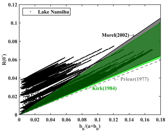
Figure 3.
Irradiance reflectance just below the surface simulated with HydroLight as a function of (N = 11,232) and the approximations of Prieur (1977) [1], Kirk (1984) [2], and Morel et al. (2002) [6] for the values of factor (black dot, our results; 0.33, Prieur’s approach; green region, Kirk’s approach; grey region, Morel’s approach).
These models primarily focused on ocean water, typically assumed to possess infinite depth, which was inapplicable to our research region (Figure 3). Our research region, Nansihu Lake, has a maximum depth of 2.33 m; the bottom sediment may affect the upwelling radiances and factor [43,44] so that the bottom reflectance must be considered in the radiative transfer model. Moreover, the composition and optical properties of inland waters are more complex than the ocean [45,46,47]; the maximum concentrations of chlorophyll-a and TSM are 22.32 mg m−3 and 31.21 mg L−1, respectively, larger than the previous ocean studies [6,7,8]. Therefore, for inland waters such as Lake Nansihu, further studies, and models based on IOPs and solar zenith angle were needed [13,48].
The spectrum of and was shown in Figure 4. The and values showed similar trends to for 16 values, 13 values, and 2 bottom reflectances at 27 stations, a total of N = 11,232 (Figure 4). The coefficient should be used if is not small with respect to rather than the factor. In this study, the backscattering coefficient at some stations was not small with respect to the absorption coefficient due to the effect of particulate (Table 1); therefore, was used rather than [6,13]. The value factor was relatively small at 400–650 nm, around 0.4, while there was a large change in factor at 650–750 nm, with a maximum value approaching 18. Therefore, those situations were separated to study.
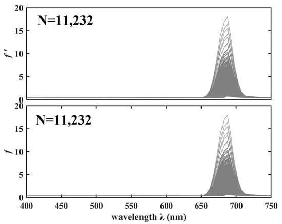
Figure 4.
The spectrum of and for finitely deep water at 27 stations in Lake Nansihu simulated with HydroLight.
Three particle phase functions, of 0.01, 0.0183, and 0.03 were used to simulate and calculate the factor in the 400–650 nm, which were often represented for the collective particle scattering research of mineral particles and phytoplankton [7,8,27,28,48,49]. At 400–650 nm, as the solar zenith angle increased, the value of the increased (Figure 5) for three values of of 0.01, 0.0183 and 0.03. It can be seen that particulate backscattering ratios had little influence on factor and can be ignored in the 400–650 nm range. Hence, we proposed an approximation of that is independent of the water body and dependent only on the solar zenith angle, . increases continuously as , rising from 0.33 to 0.43 in Figure 5. The dependence of on is approximately linear, and linear regression analysis of the data yields the relationship
Combining this relationship with Equation (1), we obtain
The coefficient of determination R2 was 0.8929, and the sum of squares of errors and root mean square error were 0.0038 and 0.0071, respectively. The results indicated that the factor increased with in a rather regular way, when ; and was linearly related to when (Figure 5). This model was similar to Kirk’s model and Morel’s approach in which or is a function of solar zenith angle.

Figure 5.
factor plotted as a function of () and the corresponding linear fit for Nansihu Lake with three particulate backscattering ratios () at 400–650 nm. R2 = 0.8929, sum of squares of errors = 0.0038, root mean square error = 0.0071. Gray circle, blue triangle, and green square represent different values of (0.01, 0.0183, and 0.03, respectively).

In the 650–750 nm range, the coefficients of determination (R2) for with and are presented in Figure 6. The factor and exhibit a large coefficient of determination (R2 0.8 at 660–710 nm), whereas is unrelated to (R2 0.0), which showed no significant linear positive correlation. Hence, we assumed that, in the range of 650–750 nm, the variation of factor mainly depends on the IOPs ( and ), and is independent of the solar zenith angle as it had little influence on the factor in the 650–750 nm (Figure 6).
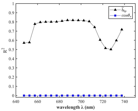
Figure 6.
Coefficients of determination (R2) for with and at 640–740 nm.
The factor had a large change with different values of and (Figure 7), and decreased with the average number of collisions () increasing. Therefore, we propose an approximation of the factor in the range of 650–750 nm with values at 600 nm divided 27 stations into six types, provided that factor is independent of and dependent on . Aside from the impact of the average number of collisions, the factor was significantly influenced by the changes in the backscattering ratios since variation in the results in changes VSFs, which ultimately affected the bidirectional reflectance distribution function [6,7]. In the 650–750 nm, factor mainly followed a Gaussian distribution, and backscattering ratios determined the height of the peak of the Gaussian function, which was not reported in previous studies since there are weakly remote-sensing reflectance in the red and near-infrared bands for the ocean waters [6,7,8,30,31]. The dependence of factor on is an approximately Gaussian function and is expressed with the equation:
where , B = 14.24 ± 0.12, C = 0.374 ± 0.016, and the coefficient was obtained from the lookup table according to the and values (Table 2). The central Gaussian function was around 685 nm, which always had a maximum of factor. The full width at the half of the maximum was about 23.71 nm according to the calculation of the value of B, which had little effect of the and values in this study. The larger the particulate backscattering ratios, the smaller the values. Thus, we can express as an explicit function of , , and the coefficient in the 650–750 nm range:
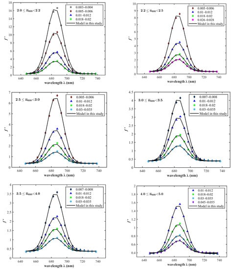
Figure 7.
The factor and the fitting model used in this study at 645–740 nm with various values and various conditions of at 600 nm.
Table 2.
Lookup table of mean A values and standard deviation as a function of at 600 nm and .
This research has shown that particle backscattering can alter the BRDF in the 650–750 nm, and values decreased as the backscattering increased. This conclusion was consistent with the findings of Loisel and Morel [13,37], which indicated an increase in backscattering leads to BRDF change from anisotropy to isotropy. However, we still do not know what the critical value of particle backscattering is. In other words, the BRDF’s impact on remote sensing must be considered in Nansihu Lake.
Mean values as a function f the solar angle, and wavelength are proposed as Equations (17) and (19), and A values obtained using Equation (19) are provided in Table 2. Detailed lookup tables for other values, including B and C, are available upon request from the authors.
The value of A, B, and C in Equation (19) will affect the accuracy of the model’s estimation of factor, especially the value of A. The smaller the values of and , the greater the uncertainties brought by the value of A (Table 2). The maximum standard deviation was around 0.25 of the value of A when the was between 2.0 and 2.2 and the was between 0.003 and 0.004, respectively. Root mean square error (RMSE) was used as an indicator of the uncertainty. The maximum error always was at 687.5 nm, as our model was and in this band, it always had a maximum. At 678.5 nm, the maximum RMSE was 0.68 when the was between 2.0 and 2.2 and the was between 0.003 and 0.004, respectively; and the minimum value was 0.01 when the was between 4.0 and 5.0 and the was between 0.045 and 0.055, respectively. The RMSE showed that the smaller the values of and , the greater the uncertainties because the factor always had a maximum value at 687.5 nm and decreased with the values of and increasing in our results. This is an important finding that has not been mentioned in previous studies [6,7,8], which focused on less than 660 nm.
To the extent that values increase as A values increase, when increases, a multiple-scattering regime develops in which the upward field tends to become isotropic and less sensitive to or VSFs, with lower values.
This study demonstrates that the factor is a function of the solar zenith angle, , and at various wavelengths under the condition of and two different bottom reflectances. It is necessary to discuss the effect of and two bottom reflectances on the study the factor. We investigated whether the concentration of CDOM had an impact on the study. Figure 8 shows the spectra at three stations (Station 10, 11, and 21) with of 0.013, 0.01, and 0.0068, respectively. CDOM absorption ranged from 0.1 to 0.9 at an interval of 0.05 at 440 nm.
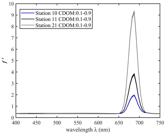
Figure 8.
spectra at 440 nm for various values from 0.1 to 0.9 at an interval of 0.05 at stations 10, 11, and 21; n = 51.
Analysis of variance (ANOVA) was used to determine the statistical significance of factor with the CDOM absorption and two bottom types, namely, seagrass and macrophytes; these reflectance spectra are shown in Figure 1a. The ANOVA showed that the impact of the magnitude of at 440 nm on factor (Table 3) was not significantly different. The values of p were equal to 1 in the three stations, indicating that the effect of on can be ignored when . The effect of dissolved colored organic substance (CDOM) on the factor can be ignored if the absorption coefficient of CDOM () is less than 0.9 at 440 nm; it was in agreement with the findings of Shen [49] in Taihu Lake. Hence, the dependence of the relationship between IOPs and AOPs on was studied under this condition.
Table 3.
ANOVA results for the effects of on the magnitude of at 440 nm. SSR and MSR represent the sum of squares regression and mean square regression, respectively.
Likewise, the values obtained for clean seagrass and macrophyte bottom reflectances are displayed in Figure 9 for various values. These had almost the same factor values across various values under the same condition.
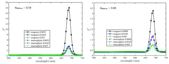
Figure 9.
spectra of average clean seagrass and macrophyte bottom reflectances for various values; and 2.13 at 600 nm, respectively.
The sum of squares regression (SSR) and mean square regression (MSR) were zero (Table 3), and the p value was equal to 1, demonstrating that the effect of two bottom reflectances was identical on the factor. However, bottom types and reflectance can affect the BRDF, and further research is neded to investigate [43].
This study shows that ƒ′ factor varied over the range of 0.33–16.64 in Lake Nansihu, a finite depth water, higher than the range observed for the ocean. The previous studies were mainly less than 660 nm [6,8,13], and the range observed for the ocean was 0.3–0.6; we had a good agreement within these ranges of previous studies, and the solar zenith is the main factor affecting the BRDF. Both of us described factor as a function of solar zenith angle and given a fitting function model. Moreover, we studied a wider range wavelength than the previous studies, 660–750 nm. we found that factor mainly followed a Gaussian distribution in the 650–750 nm, and the range of 0.33–16.64 in the 650–750 nm, which was less mentioned in previous studies. There was less research on the relationship between VSFs and BRDF, because of a lack of measurement of VSFs [7]. In our study, the VSFs was characterized by particulate backscattering ratios, which is more easily obtained. Our results indicated the larger the particulate backscattering ratios, the smaller the values. Additionally, the central of Gaussian function was around 685 nm, which always had a maximum of factor, and backscattering ratios determined the height of the peak of the Gaussian function. These findings and models can compensate for the shortcomings of factor research in the red and near infrared bands and improve the ability of modeling the irradiance distribution in inland waters. However, our studies were based on the chlorophyll-a and TSM concentrations ranging from 5.00 to 22.32 mg m−3 and from 1.02 to 31.21 mg L−1, respectively. For inland turbid waters, TSM concentration is more higher than our study region [50,51,52], with TSM > 100 mg L−1; the extremely turbid waters are perfectly diffuse scattering bodies, which leads to isotropy [13]. Hence, further research is needed to investigate the BRDF of turbid inland waters.
4. Conclusions
The ƒ′ factor of BRDF serves as a crucial connection between the IOPs and AOPs of inland waters. In this study, the radiative transfer model was applied to calculate the ƒ′ values, taking into account the finite depth. This study reveals that the behavior of photons in inland waters results from the combined effects of the solar angle, VSFs, and optically shallow bottoms. Two parametric models were proposed to evaluate ƒ′ values, with one as a function of solar angle in the 400–650 nm, and the other model of and and wavelength in the range of 650–750 nm. It was found that the ƒ′ has a continuous geometric increase as the value of increases. However, it is relatively insensitive to solar angles in the 650–750 nm range. For this range, mainly follows a Gaussian function related to and and wavelength with the reference wavelength . In Lake Nansihu, the larger the scattering and backscattering, the smaller the ƒ′ factor values. In the future, measurement of in-water irradiance reflectance and IOPs will be necessary to validate the model and assessment of at various wavelengths in inland waters.
Author Contributions
Conceptualization, L.Z. and Y.Z.; methodology, Y.Z.; software, L.Z.; validation, Q.T., C.H. and Y.C.; formal analysis, Y.Z.; data curation, C.H.; writing—original draft preparation, L.Z. and Y.Z.; writing—review and editing, C.H. and Y.C.; supervision, Q.T.; project administration, L.Z.; funding acquisition, L.Z. All authors have read and agreed to the published version of the manuscript.
Funding
This research was funded by the National Natural Science Foundation of China, grant number 41830108.
Data Availability Statement
The data presented in this study are available on request from the corresponding author.
Conflicts of Interest
The authors declare no conflict of interest.
References
- Morel, A.; Prieur, L. Analysis of Variations in Ocean Color1: Ocean Color Analysis. Limnol. Oceanogr. 1977, 22, 709–722. [Google Scholar] [CrossRef]
- Kirk, J.T.O. Dependence of Relationship Between Inherent and Apparent Optical Properties of Water on Solar Altitude. Limnol. Oceanogr. 1984, 29, 350–356. [Google Scholar] [CrossRef]
- Gordon, H.R. Dependence of the Diffuse Reflectance of Natural Waters on the Sun Angle. Limnol. Oceanogr. 1989, 34, 1484–1489. [Google Scholar] [CrossRef]
- Gordon, H.R.; Brown, O.B.; Jacobs, M.M. Computed Relationships Between the Inherent and Apparent Optical Properties of a Flat Homogeneous Ocean. Appl. Opt. 1975, 14, 417. [Google Scholar] [CrossRef] [PubMed]
- Højerslev, N.K. Analytic Remote-Sensing Optical Algorithms Requiring Simple and Practical Field Parameter Inputs. Appl. Opt. 2001, 40, 4870. [Google Scholar] [CrossRef] [PubMed]
- Morel, A.; Antoine, D.; Gentili, B. Bidirectional Reflectance of Oceanic Waters: Accounting for Raman Emission and Varying Particle Scattering Phase Function. Appl. Opt. 2002, 41, 6289. [Google Scholar] [CrossRef]
- He, S.; Zhang, X.; Xiong, Y.; Gray, D. A Bidirectional Subsurface Remote Sensing Reflectance Model Explicitly Accounting for Particle Backscattering Shapes. JGR Oceans 2017, 122, 8614–8626. [Google Scholar] [CrossRef]
- Lee, Z.P.; Du, K.; Voss, K.J.; Zibordi, G.; Lubac, B.; Arnone, R.; Weidemann, A. An Inherent-Optical-Property-Centered Approach to Correct the Angular Effects in Water-Leaving Radiance. Appl. Opt. 2011, 50, 3155. [Google Scholar] [CrossRef]
- Zhai, P.-W.; Hu, Y.; Trepte, C.R.; Winker, D.M.; Lucker, P.L.; Lee, Z.; Josset, D.B. Uncertainty in the Bidirectional Reflectance Model for Oceanic Waters. Appl. Opt. 2015, 54, 4061. [Google Scholar] [CrossRef]
- Morel, A.; Mueller, J.L. Normalized Water-Leaving Radiance and Remote Sensing Reflectance: Bidirectional Reflectance and Other Factors. In Ocean Optics Protocols For Satellite Ocean Color Sensor Validation; Revision 3; National Aeronautics and Space Administration, Goddard Space Flight Center: Greenbelt, MD, USA, 2002; pp. 183–210. [Google Scholar]
- Kirk, J.T.O. Volume Scattering Function, Average Cosines, and the Underwater Light Field. Limnol. Oceanogr. 1991, 36, 455–467. [Google Scholar] [CrossRef]
- Morel, A.; Gentili, B. Diffuse Reflectance of Oceanic Waters: Its Dependence on Sun Angle as Influenced by the Molecular Scattering Contribution. Appl. Opt. 1991, 30, 4427. [Google Scholar] [CrossRef] [PubMed]
- Loisel, H.; Morel, A. Non-Isotropy of the Upward Radiance Field in Typical Coastal (Case 2) Waters. Int. J. Remote Sens. 2001, 22, 275–295. [Google Scholar] [CrossRef]
- Chami, M.; Thirouard, A.; Harmel, T. POLVSM (Polarized Volume Scattering Meter) Instrument: An Innovative Device to Measure the Directional and Polarized Scattering Properties of Hydrosols. Opt. Express 2014, 22, 26403. [Google Scholar] [CrossRef] [PubMed]
- Harmel, T. Recent Developments in the Use of Light Polarization for Marine Environment Monitoring from Space. In Light Scattering Reviews 10; Springer: Berlin/Heidelberg, Germany, 2016; pp. 41–84. ISBN 978-3-662-46761-9. [Google Scholar]
- Twardowski, M.; Tonizzo, A. Ocean Color Analytical Model Explicitly Dependent on the Volume Scattering Function. Appl. Sci. 2018, 8, 2684. [Google Scholar] [CrossRef]
- Mobley, C.D.; Sundman, L.K.; Boss, E. Phase Function Effects on Oceanic Light Fields. Appl. Opt. 2002, 41, 1035. [Google Scholar] [CrossRef] [PubMed]
- Fournier, G.R.; Forand, J.L. Analytic Phase Function for Ocean Water; Jaffe, J.S., Ed.; SPIE: Bergen, Norway, 1994; pp. 194–201. [Google Scholar]
- Whitmire, A.L.; Boss, E.; Cowles, T.J.; Pegau, W.S. Spectral Variability of the Particulate Backscattering Ratio. Opt. Express 2007, 15, 7019. [Google Scholar] [CrossRef]
- Gordon, H.R.; Smyth, T.J.; Balch, W.M.; Boynton, G.C.; Tarran, G.A. Light Scattering by Coccoliths Detached from Emiliania Huxleyi. Appl. Opt. 2009, 48, 6059. [Google Scholar] [CrossRef]
- Boss, E. Particulate Backscattering Ratio at LEO 15 and Its Use to Study Particle Composition and Distribution. J. Geophys. Res. 2004, 109, C01014. [Google Scholar] [CrossRef]
- McKee, D.; Cunningham, A. Identification and Characterisation of Two Optical Water Types in the Irish Sea from in Situ Inherent Optical Properties and Seawater Constituents. Estuar. Coast. Shelf Sci. 2006, 68, 305–316. [Google Scholar] [CrossRef]
- Loisel, H.; Mériaux, X.; Berthon, J.-F.; Poteau, A. Investigation of the Optical Backscattering to Scattering Ratio of Marine Particles in Relation to Their Biogeochemical Composition in the Eastern English Channel and Southern North Sea. Limnol. Oceanogr. 2007, 52, 739–752. [Google Scholar] [CrossRef]
- Snyder, W.A.; Arnone, R.A.; Davis, C.O.; Goode, W.; Gould, R.W.; Ladner, S.; Lamela, G.; Rhea, W.J.; Stavn, R.; Sydor, M.; et al. Optical Scattering and Backscattering by Organic and Inorganic Particulates in US Coastal Waters. Appl. Opt. 2008, 47, 666. [Google Scholar] [CrossRef]
- Gordon, H.R.; Lewis, M.R.; McLean, S.D.; Twardowski, M.S.; Freeman, S.A.; Voss, K.J.; Boynton, G.C. Spectra of Particulate Backscattering in Natural Waters. Opt. Express 2009, 17, 16192. [Google Scholar] [CrossRef]
- Soja-Woźniak, M.; Baird, M.; Schroeder, T.; Qin, Y.; Clementson, L.; Baker, B.; Boadle, D.; Brando, V.; Steven, A.D.L. Particulate Backscattering Ratio as an Indicator of Changing Particle Composition in Coastal Waters: Observations From Great Barrier Reef Waters. J. Geophys. Res. Oceans 2019, 124, 5485–5502. [Google Scholar] [CrossRef]
- Sun, D.; Su, X.; Wang, S.; Qiu, Z.; Ling, Z.; Mao, Z.; He, Y. Variability of Particulate Backscattering Ratio and Its Relations to Particle Intrinsic Features in the Bohai Sea, Yellow Sea, and East China Sea. Opt. Express 2019, 27, 3074. [Google Scholar] [CrossRef]
- Kheireddine, M.; Brewin, R.J.W.; Ouhssain, M.; Jones, B.H. Particulate Scattering and Backscattering in Relation to the Nature of Particles in the Red Sea. J. Geophys. Res. Oceans 2021, 126, e2020JC016610. [Google Scholar] [CrossRef]
- Petzold, T.J. Volume Scattering Functions for Selected Ocean Waters; Defense Technical Information Center: Fort Belvoir, VA, USA, 1972. [Google Scholar]
- Mobley, C.D.; Gentili, B.; Gordon, H.R.; Jin, Z.; Kattawar, G.W.; Morel, A.; Reinersman, P.; Stamnes, K.; Stavn, R.H. Comparison of Numerical Models for Computing Underwater Light Fields. Appl. Opt. 1993, 32, 7484. [Google Scholar] [CrossRef]
- Morel, A.; Gentili, B. Diffuse Reflectance of Oceanic Waters III Implication of Bidirectionality for the Remote-Sensing Problem. Appl. Opt. 1996, 35, 4850. [Google Scholar] [CrossRef]
- Bricaud, A.; Morel, A.; Babin, M.; Allali, K.; Claustre, H. Variations of Light Absorption by Suspended Particles with Chlorophyll a Concentration in Oceanic (Case 1) Waters: Analysis and Implications for Bio-Optical Models. J. Geophys. Res. 1998, 103, 31033–31044. [Google Scholar] [CrossRef]
- Pope, R.M.; Fry, E.S. Absorption Spectrum (380–700 Nm) of Pure Water II Integrating Cavity Measurements. Appl. Opt. 1997, 36, 8710. [Google Scholar] [CrossRef]
- Prieur, L.; Sathyendranath, S. An Optical Classification of Coastal and Oceanic Waters Based on the Specific Spectral Absorption Curves of Phytoplankton Pigments, Dissolved Organic Matter, and Other Particulate Materials1: Optical Classification. Limnol. Oceanogr. 1981, 26, 671–689. [Google Scholar] [CrossRef]
- Ahn, Y.-H. Proprietes Optiques Des Particules Biologiques et Minerales Presentes Dans l’ocean. Application: Inversion de La Reflectance. Ph.D. Thesis, Universite Pierre et Marie Curie, Paris, France, 1990; 214p. [Google Scholar]
- Bricaud, A.; Morel, A.; Prieur, L. Absorption by Dissolved Organic Matter of the Sea (Yellow Substance) in the UV and Visible Domains. Limnol. Oceanogr. 1981, 26, 43–53. [Google Scholar] [CrossRef]
- Loisel, H.; Morel, A. Light Scattering and Chlorophyll Concentration in Case 1 Waters: A Reexamination. Limnol. Oceanogr. 1998, 43, 847–858. [Google Scholar] [CrossRef]
- Chami, M.; Marken, E.; Stamnes, J.J.; Khomenko, G.; Korotaev, G. Variability of the Relationship between the Particulate Backscattering Coefficient and the Volume Scattering Function Measured at Fixed Angles. J. Geophys. Res. 2006, 111, C05013. [Google Scholar] [CrossRef]
- Zhang, X.; Hu, L.; He, M.-X. Scattering by Pure Seawater: Effect of Salinity. Opt. Express 2009, 17, 5698. [Google Scholar] [CrossRef] [PubMed]
- Jeffrey, S.W.; Humphrey, G.F. New Spectrophotometric Equations for Determining Chlorophylls a, b, C1 and C2 in Higher Plants, Algae and Natural Phytoplankton. Biochem. Physiol. Pflanz. 1975, 167, 191–194. [Google Scholar] [CrossRef]
- Harrison, A.W.; Coombes, C.A. Angular Distribution of Clear Sky Short Wavelength Radiance. Sol. Energy 1988, 40, 57–63. [Google Scholar] [CrossRef]
- Kasten, F.; Czeplak, G. Solar and Terrestrial Radiation Dependent on the Amount and Type of Cloud. Sol. Energy 1980, 24, 177–189. [Google Scholar] [CrossRef]
- Mobley, C.D.; Zhang, H.; Voss, K.J. Effects of Optically Shallow Bottoms on Upwelling Radiances: Bidirectional Reflectance Distribution Function Effects. Limnol. Oceanogr. 2003, 48, 337–345. [Google Scholar] [CrossRef]
- Lee, Z.; Carder, K.L.; Mobley, C.D.; Steward, R.G.; Patch, J.S. Hyperspectral Remote Sensing for Shallow Waters: 2 Deriving Bottom Depths and Water Properties by Optimization. Appl. Opt. 1999, 38, 3831. [Google Scholar] [CrossRef]
- Spyrakos, E.; O’Donnell, R.; Hunter, P.D.; Miller, C.; Scott, M.; Simis, S.G.H.; Neil, C.; Barbosa, C.C.F.; Binding, C.E.; Bradt, S.; et al. Optical Types of Inland and Coastal Waters: Optical Types of Inland and Coastal Waters. Limnol. Oceanogr. 2018, 63, 846–870. [Google Scholar] [CrossRef]
- Seegers, B.N.; Werdell, P.J.; Vandermeulen, R.A.; Salls, W.; Stumpf, R.P.; Schaeffer, B.A.; Owens, T.J.; Bailey, S.W.; Scott, J.P.; Loftin, K.A. Satellites for Long-Term Monitoring of Inland U.S. Lakes: The MERIS Time Series and Application for Chlorophyll-a. Remote Sens. Environ. 2021, 266, 112685. [Google Scholar] [CrossRef]
- Kutser, T.; Vahtmäe, E.; Paavel, B.; Kauer, T. Removing Glint Effects from Field Radiometry Data Measured in Optically Complex Coastal and Inland Waters. Remote Sens. Environ. 2013, 133, 85–89. [Google Scholar] [CrossRef]
- Gleason, A.C.R.; Voss, K.J.; Gordon, H.R.; Twardowski, M.; Sullivan, J.; Trees, C.; Weidemann, A.; Berthon, J.-F.; Clark, D.; Lee, Z.-P. Detailed Validation of the Bidirectional Effect in Various Case I and Case II Waters. Opt. Express 2012, 20, 7630. [Google Scholar] [CrossRef]
- Qian, S. Bi-Directional Properties of Light Field of Inland Waters Based on Simulated Data by Hydrolight. J. Beijing Univ. Technol. 2017, 43, 649–658. [Google Scholar] [CrossRef]
- Le, C.; Li, Y.; Zha, Y.; Sun, D.; Huang, C.; Lu, H. A Four-Band Semi-Analytical Model for Estimating Chlorophyll a in Highly Turbid Lakes: The Case of Taihu Lake, China. Remote Sens. Environ. 2009, 113, 1175–1182. [Google Scholar] [CrossRef]
- Knaeps, E.; Ruddick, K.G.; Doxaran, D.; Dogliotti, A.I.; Nechad, B.; Raymaekers, D.; Sterckx, S. A SWIR Based Algorithm to Retrieve Total Suspended Matter in Extremely Turbid Waters. Remote Sens. Environ. 2015, 168, 66–79. [Google Scholar] [CrossRef]
- Liu, G.; Li, L.; Song, K.; Li, Y.; Lyu, H.; Wen, Z.; Fang, C.; Bi, S.; Sun, X.; Wang, Z.; et al. An OLCI-Based Algorithm for Semi-Empirically Partitioning Absorption Coefficient and Estimating Chlorophyll a Concentration in Various Turbid Case-2 Waters. Remote Sens. Environ. 2020, 239, 111648. [Google Scholar] [CrossRef]


Disclaimer/Publisher’s Note: The statements, opinions and data contained in all publications are solely those of the individual author(s) and contributor(s) and not of MDPI and/or the editor(s). MDPI and/or the editor(s) disclaim responsibility for any injury to people or property resulting from any ideas, methods, instructions or products referred to in the content. |
© 2023 by the authors. Licensee MDPI, Basel, Switzerland. This article is an open access article distributed under the terms and conditions of the Creative Commons Attribution (CC BY) license (https://creativecommons.org/licenses/by/4.0/).